


Abstract
GS 1826−238 is a well-studied low-mass X-ray binary neutron star. This source was in a persistent hard state since its discovery in 1988 and until 2014 June. After that, the source exhibited several softer periods of enhanced intensity in the energy range 2–20 keV. We studied the long-term light curves of MAXI (Monitor of All Sky X-ray Image) and Swift/BAT, and found clearly two branches in the MAXI–BAT and hardness–intensity diagrams, which correspond to the persistent state and softer periods, respectively. We analysed 21 Swift/XRT observations, of which four were located in the persistent state while the others were in softer periods or in a state between them. The XRT spectra could be generally fitted by using an absorbed Comptonization model with no other components required. We found a peculiar relationship between the luminosity and the hardness in the energy range of 0.6–10 keV: when the luminosity is larger (smaller) than 4 per cent–6 per cent Ledd, the hardness is anti-correlated (correlated) with luminosity. We also estimated the variability for each observation by using the fractional rms in the 0.1–10 Hz range. We found that the observations in the persistent state had a large fractional rms of ∼25 per cent, similar to other low-mass X-ray binaries. However, the variability is mainly found in the range of 5 per cent–20 per cent during softer periods. We suggest that GS 1826−238 did not evolve into the soft state of atoll sources, and all the observed XRT observations during the softer periods resemble a peculiar intermediate state of atoll sources.
1 INTRODUCTION
A low-mass X-ray binary (LMXB) is a system with either a neutron star (NS) or a black hole accreting material from a stellar-mass donor star, usually via Roche lobe overflow. GS 1826−238 is a well-known NS in an LMXB system discovered with Ginga in 1988 (Makino 1988). It was reported in a persistent hard state from its discovery until 2014 June. After that, Nakahira et al. (2014) and Asai et al. (2015) found that the source had moved to the first of several ‘softer periods’ (SPs) characterized by softer spectra and enhanced flux in the 2–20 keV range, as seen in the MAXI light curve for count rates ≳0.2 counts s−1 (Palmer & Swift/BAT Team 2017). In this paper, we refer to these periods as ‘SPs’. A quasi-periodicity of type-I X-ray bursts observed during the persistent hard state has been reported by Ubertini et al. (1999). Burst profiles have been found to be extremely stable (see fig. 2 in Galloway et al. 2004), making GS 1826−238 the ‘clocked’ burster. A hard X-ray shortage above 30 keV during bursts was reported, which was suggested as the coronal Compton cooling via the burst emission (Ji et al. 2014, 2015). After the transition in 2014, Chenevez et al. (2016) found that burst profiles and the recurrence time varied significantly, ruling out the regular bursts that were typical for this source in the persistent state.
In general, LMXBs can be approximately classified as either Z-sources or atoll sources, based on their traces in the colour–colour diagram (CCD) or the hardness–intensity diagram (HID; for details, see Lewin & van der Klis 2006). Another important tool that can be used to study the outburst evolution is the root-mean-square (rms)–intensity diagram (Muñoz-Darias, Motta & Belloni 2011; Muñoz-Darias et al. 2014). Muno, Remillard & Chakrabarty (2002) tentatively classified GS 1826−238 as an atoll source, although there was only a little variability in the CCD.
Thompson et al. (2008) also obtained a similar result, and claimed that all the observations seemed to be located in the hard state that typically characterizes atoll LMXBs.
In LMXBs, there are three canonical states, i.e. the low/hard state, the high/soft state and the intermediate state (Remillard & McClintock 2006). In the soft state, the spectrum is dominated by a thermal component and the fractional rms is usually <5 per cent (Muñoz-Darias et al. 2011, 2014). In the hard state, the spectrum is dominated by a power-law component (|$\frac{{\rm d}N}{{\rm d}E}\propto E^{-\Gamma }$|) with a Γ of 1.4–2.1, and the fractional rms is ≳20 per cent. In the intermediate state, the thermal and power-law components are comparable, and the fractional rms is ∼5 per cent–20 per cent. It is widely believed that the thermal component originates from the accretion disc, the surface of the NS and the boundary between them. In contrast, the power-law component is thought to originate from hot plasmas above the accretion disc or within the innermost radius of the accretion disc, the so-called corona, or from jets (Frank, King & Raine 2002). The intermediate state, which is regarded as the transition between the hard and soft state, reflects the change of the accretion region (see e.g. Esin, McClintock & Narayan 1997; Done, Gierliński & Kubota 2007), of which the detailed process is still poorly known (Begelman 2014).
The spectrum of GS 1826−238 is well studied since the source remained in the persistent state for tens of years, with a stable hard spectrum, before the onset of the SP in 2014. In general, its broad-band X-ray spectrum can be successfully described as a combination of two Comptonization components based on Chandra, XMM–Newton, BeppoSAX, INTEGRAL and RXTE observations. The physical scenario is however still debated (Thompson et al. 2005, 2008; Cocchi, Farinelli & Paizis 2011; Ono et al. 2016). When the statistics of the data quality is not good enough, the spectrum can be described by a simplified model including only one Comptonization component successfully (in’t Zand et al. 1999; Cocchi et al. 2010). In addition, a significant high-energy (>150 keV) excess above the Comptonization models is found (Rodi, Jourdain & Roques 2016). During the SP in 2014, the source's spectrum evolved into a softer episode, whose spectrum observed by Swift and NuSTAR could be still described using a dual Comptonization model (Chenevez et al. 2016). However, we note that how the spectral parameters evolve in SPs is still unclear and addressed in the literature. Therefore, in this paper, we analysed archived MAXI and Swift data of GS 1826−238 to investigate the spectral evolution and the light-curve variability of the source in the SPs.
2 OBSERVATIONS AND DATA ANALYSIS
2.1 MAXI
The Gas Slit Camera on board the Monitor of All Sky X-ray Image (MAXI; Matsuoka et al. 2009) has been monitoring GS 1826−238 since the beginning of the mission. We used publicly daily averaged light curves in three energy ranges, i.e. 2–4, 4–10 and 2–20 keV, in the following analysis.1 We did not use the light curve in the energy range of 10–20 keV because of the low signal-to-noise ratio. We removed observations when the source's flux is negative, most likely because of systematic errors.
2.2 Swift
We adopted the daily averaged 15–50 keV light curve measured by BAT to describe the long-term evolution of GS 1826−238 at hard X-rays during SPs (Barthelmy et al. 2005). We also analysed 21 XRT (Burrows et al. 2005) observations, in which only the windowed timing (WT) data were considered (see Table 1). The XRT data were processed with standard procedures xrtpipeline, following the official User's Guide.2 Our analysis was performed by using heasoft v.6.20 with the latest CALDB files. Before spectral fits, the extracted spectra were grouped in order to have more than 25 counts per bin. During spectral fittings, the energy range adopted was 0.6–10 keV. All the uncertainties quoted are at 90 per cent confidence level.
3 RESULTS
3.1 Long-term light curves
We show the long-term MAXI (2–20 keV) and BAT (15–50 keV) light curves in Fig. 1. Before MJD 56500, the light curves are quite stable, only showing weak fluctuations. An increase of soft X-rays around MJD ∼ 56700 is observed, accompanied by a significant reduction of the emission at hard X-rays. After that, several bright SPs were detected in the soft X-ray band (shown in Fig. 1), during which the hard X-rays showed a large and complex variability.
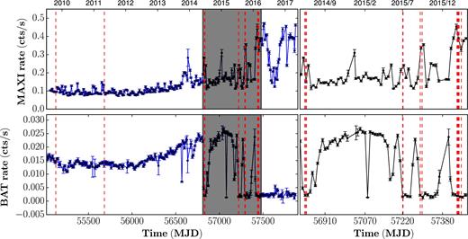
Left two panels: long-term light curves as measured by MAXI (2–20 keV) and Swift/BAT (15–50 keV) with a bin size of 10 d. The red lines represent the time of Swift/XRT observations. We note that two XRT observations (first two rows in Table 1) are not included in this figure because of the lack of MAXI data before 2009. Right two panels: a zoom of SPs. We show this duration in the left-hand panels by using a dark shadow.
To understand the relation between soft and hard X-rays, we show the count rates of MAXI and BAT in Fig. 2 (upper panel) for the time interval shown in Fig. 1. In practice, we only selected the MAXI–BAT pairs if the difference of their observed time was less than 1 d. Clearly, two branches are observed: (1) when the MAXI count rate is larger than 0.2, corresponding to ∼60.6 mCrab,3 and the hard X-rays are very faint; (2) when the MAXI count rate is smaller than 0.2 counts s−1 and the BAT intensity changes drastically with almost a constant soft X-ray level.
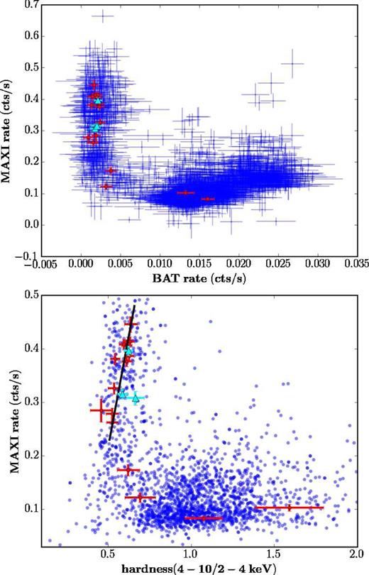
Upper panel: daily averaged Swift/BAT (15–50 keV) count rates versus the corresponding MAXI (2–20 keV) count rates. Lower panel: the HID, where the hardness is defined as the ratio of the MAXI count rate between 4–10 and 2–4 keV, and the intensity is described as the MAXI count rate in the 2–20 keV energy band. The red markers represent the pointing XRT observations. The cyan triangle markers represent the observations in 00035342012, 00035342019 and 00035342024, in which the absorbed Comptonization model leads to relatively poor fittings (see the text). The black line shows a linear fitting of XRT observations when the MAXI rate is larger than 0.2 counts s−1.
For the same time interval, we also show the HID in the lower panel of Fig. 2, where the hardness is defined as the ratio of the count rates between 4–10 and 2–4 keV. In this diagram, when the MAXI count rate is larger than 0.2 counts s−1, the source is in a relatively soft state, i.e. a small hardness value. However, it seems that the hardness tends to increase slightly with the increase of the soft X-ray intensity (this result will be further verified in the following analysis). When the MAXI count rate is smaller than 0.2 counts s−1, the hardness is significantly larger and changes drastically within a narrow range of soft X-rays.
We also analysed 21 pointed XRT observations performed at the times shown in Fig. 1 with dashed red vertical lines. We estimated their locations in Fig. 2 by averaging five nearest MAXI and BAT observations. Clearly, most of the XRT observations are located in the SPs with different flux levels, and only four observations are in the intermediate or hard state. We used a linear function to fit the relation between the hardness and MAXI rate of these XRT observations when the MAXI rate is larger than 0.2 counts s−1 (shown in Fig. 2).
We found that the hardness increases with the MAXI rate at 3.6σ confidence level. Here we note that there are two additional XRT observations that are also in the hard state, but are not included in Figs 1 and 2 because of the lack of MAXI observations before 2009. Since GS 1826−238 was observed in different stages during SPs, it allows us for the first time to investigate the evolution of different states with unprecedented data in this source.
3.2 Spectral and variability properties
We extracted XRT spectra with standard event grades 0–2 for WT mode. Type-I bursts were filtered out to avoid the contamination of the persistent emission. We tried to fit the spectra by using an xspec model ‘tbabs*nthcomp’, where the ‘tbabs’ component was used to describe the absorption caused by the interstellar medium (Wilms, Allen & McCray 2000) and the ‘nthcomp’ component represented the thermally Comptonized continuum (Zdziarski, Johnson & Magdziarz 1996; Życki, Done & Smith 1999). There are five parameters in the ‘nthcomp’ component, i.e. the asymptotic power-law photon index (Γ), the electron temperature (Te), the seed photon temperature (Tbb), the inp_type (blackbody or disc-blackbody seed photons) and the normalization. In this work, we assumed blackbody seed photons, i.e. inp_type = 0. Te, which corresponds to the high-energy rollover at E ∼ 2 Te, could not be constrained by using XRT data. Therefore, we fixed it at Te = 21 keV, based on Thompson et al. (2005). Although the reduction of Te has been reported in Cocchi et al. (2011), we verified that a lower Te would not change our findings. We show the fitting results in Fig. 3 and Table 1. We found that in general a single Comptonization model could describe the XRT data very well. The null hypothesis probability4 is >0.01 (except for three out of 21 observations, i.e. 00035342012, 00035342019 and 00035342024), which means that no additional components, e.g. a soft blackbody proposed by in’t Zand et al. (1999) or another Comptonization component (Thompson et al. 2005), are necessary. The relatively bad fittings for the remaining three observations might originate from the oversimplified model or the intrinsic variability of the spectra (Chenevez et al. 2016). We tried to add an extra blackbody or disc-blackbody to fit these three spectra; however, they could not improve the fitting quality. An extra Comptonization model could improve the fitting significantly, but this is not surprising because of having higher degree of freedom, and the resulting parameters cannot be well constrained. Actually, even for the observations with null hypothesis probability of <0.01, some residuals were only shown at soft X-rays (<2–3 keV). Therefore, the ‘tbabs*nthcomp’ model is good enough to describe the spectral shape approximately. In order to compare fitting results in different observations, in this paper we only adopted the single Comptonization model.
Fitting parameters by using the ‘tbabs*nthcomp’ model in GS 1826−238. The flux is estimated in the 0.6–10 keV band.
Spectral fitting parameters of XRT observations for GS 1826−238 by using a ‘tbabs*nthcomp’ model.
| Obs | Time | Texpo | NH | Γ | kTbb | Reduced-χ2 (dof) | Flux (0.6–10 keV) |
|---|---|---|---|---|---|---|---|
| (MJD) | (s) | (1022 cm− 2) | (keV) | (10− 9 erg s− 1 cm− 2) | |||
| 00035342001 | 53811 | 2336 | |$0.06^{0.02}_{-0.02}$| | |$1.59^{0.05}_{-0.05}$| | |$0.53^{0.03}_{-0.03}$| | 1.00 (620) | |$1.12^{0.08}_{-0.08}$| |
| 00035342002 | 53949 | 2006 | |$0.04^{0.02}_{-0.02}$| | |$1.77^{0.08}_{-0.11}$| | |$0.67^{0.04}_{-0.04}$| | 0.88 (528) | |$1.07^{0.08}_{-0.07}$| |
| 00035342004 | 55125 | 2991 | |$0.14^{0.02}_{-0.03}$| | |$1.66^{0.06}_{-0.08}$| | |$0.62^{0.04}_{-0.04}$| | 1.00 (524) | |$0.90^{0.08}_{-0.06}$| |
| 00091108001 | 55682 | 4737 | |$0.16^{0.02}_{-0.02}$| | |$1.70^{0.05}_{-0.06}$| | |$0.63^{0.03}_{-0.03}$| | 0.98 (626) | |$0.82^{0.06}_{-0.05}$| |
| 00035342005 | 56828 | 997 | |$0.18^{0.02}_{-0.02}$| | |$2.67^{0.08}_{-0.09}$| | |$0.51^{0.02}_{-0.02}$| | 0.96 (535) | |$2.92^{0.13}_{-0.19}$| |
| 00035342006 | 56832 | 15 819 | |$0.22^{0.01}_{-0.01}$| | |$2.49^{0.02}_{-0.02}$| | |$0.44^{0.01}_{-0.01}$| | 0.98 (757) | |$2.27^{0.05}_{-0.06}$| |
| 00080751002 | 56835 | 1498 | |$0.20^{0.02}_{-0.02}$| | |$2.47^{0.07}_{-0.06}$| | |$0.42^{0.02}_{-0.02}$| | 1.00 (481) | |$1.96^{0.14}_{-0.15}$| |
| 00035342007 | 57220 | 1780 | |$0.30^{0.01}_{-0.01}$| | |$2.61^{0.05}_{-0.05}$| | |$0.48^{0.01}_{-0.01}$| | 0.91 (622) | |$3.45^{0.15}_{-0.15}$| |
| 00035342009 | 57222 | 1643 | |$0.17^{0.01}_{-0.01}$| | |$2.52^{0.06}_{-0.06}$| | |$0.51^{0.01}_{-0.01}$| | 1.00 (613) | |$3.35^{0.11}_{-0.14}$| |
| 00035342011 | 57291 | 1702 | |$0.30^{0.01}_{-0.02}$| | |$2.54^{0.05}_{-0.05}$| | |$0.48^{0.01}_{-0.01}$| | 0.96 (619) | |$3.54^{0.14}_{-0.18}$| |
| 00035342012 | 57298 | 596 | |$0.39^{0.03}_{-0.04}$| | |$2.38^{0.08}_{-0.09}$| | |$0.48^{0.03}_{-0.03}$| | 1.22 (484) | |$4.05^{0.34}_{-0.37}$| |
| 00035342013 | 57437 | 989 | |$0.21^{0.02}_{-0.01}$| | |$2.46^{0.06}_{-0.07}$| | |$0.53^{0.01}_{-0.02}$| | 0.83 (603) | |$4.38^{0.19}_{-0.21}$| |
| 00035342016 | 57439 | 915 | |$0.28^{0.03}_{-0.04}$| | |$2.19^{0.09}_{-0.10}$| | |$0.52^{0.03}_{-0.03}$| | 0.96 (527) | |$5.85^{0.55}_{-0.62}$| |
| 00035342017 | 57440 | 843 | |$0.32^{0.02}_{-0.02}$| | |$2.23^{0.05}_{-0.05}$| | |$0.49^{0.02}_{-0.02}$| | 1.07 (596) | |$4.55^{0.30}_{-0.32}$| |
| 00035342018 | 57441 | 824 | |$0.30^{0.02}_{-0.02}$| | |$2.34^{0.06}_{-0.06}$| | |$0.50^{0.02}_{-0.02}$| | 1.09 (585) | |$4.37^{0.23}_{-0.23}$| |
| 00035342019 | 57442 | 945 | |$0.33^{0.02}_{-0.02}$| | |$1.97^{0.04}_{-0.04}$| | |$0.51^{0.02}_{-0.02}$| | 1.20 (655) | |$6.03^{0.29}_{-0.31}$| |
| 00035342020 | 57443 | 969 | |$0.27^{0.01}_{-0.02}$| | |$2.15^{0.05}_{-0.05}$| | |$0.53^{0.02}_{-0.02}$| | 1.03 (638) | |$5.49^{0.27}_{-0.26}$| |
| 00035342021 | 57444 | 246 | |$0.24^{0.03}_{-0.03}$| | |$2.12^{0.08}_{-0.10}$| | |$0.52^{0.03}_{-0.04}$| | 1.05 (448) | |$5.21^{0.49}_{-0.55}$| |
| 00035342022 | 57445 | 948 | |$0.33^{0.02}_{-0.02}$| | |$2.07^{0.05}_{-0.05}$| | |$0.50^{0.02}_{-0.02}$| | 1.05 (614) | |$7.88^{0.48}_{-0.55}$| |
| 00035342023 | 57446 | 972 | |$0.18^{0.01}_{-0.01}$| | |$2.32^{0.06}_{-0.06}$| | |$0.55^{0.01}_{-0.01}$| | 0.97 (611) | |$4.85^{0.23}_{-0.19}$| |
| 00035342024 | 57455 | 2726 | |$0.29^{0.01}_{-0.01}$| | |$2.20^{0.03}_{-0.03}$| | |$0.52^{0.01}_{-0.01}$| | 1.16 (725) | |$4.83^{0.16}_{-0.17}$| |
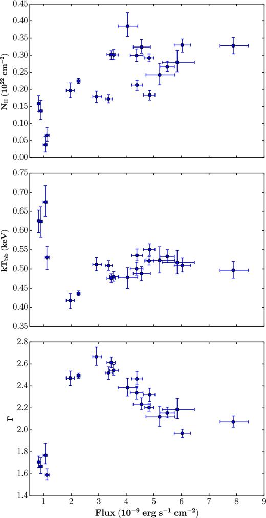
As shown in Fig. 3, the NH parameter is significantly variable. The Tbb parameter is anti-correlated with the flux (F) when F < Fc (where Fc is ∼ 2 × 10− 9 erg s− 1 cm− 2) and is approximately constant at a higher flux level. Here we estimated the flux by using the xspec command ‘flux’ in the energy range of 0.6–10 keV. The Γ, instead, is correlated with F when F < Fc and tends to be anti-correlated with F when F > Fc. The Γ describes the slope of the spectrum, i.e. the hardness. Therefore, results in Fig. 3 indicate that when the flux increases, the spectrum becomes softer if F < Fc, and harder when F > Fc. As examples, we show unfolded spectra in different regimes in Fig. 4. This result is fully consistent with the evolution pattern of the HID.
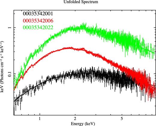
Examples of unfolded spectra of XRT observations. The black, green and red lines represent the persistent hard state, the SP and a state between them, respectively. Their spectral parameters are shown in Table 1.
We calculated the fractional rms of these XRT observations (shown in Fig. 5). We split the background-corrected light curves into contiguous segments of 51.2 s (1024 bins in each segment) and calculated the periodograms by using the ‘squared-rms’ normalization (Belloni & Hasinger 1990). The fractional rms was obtained by integrating the power spectrum density (PSD) over 0.1–10 Hz after subtracting the white noise. Since the observed periodogram is a random realization of the underlying PSD, we estimated the error of the fractional rms by evaluating the standard deviation of the power for each segment. Fig. 5 indicates that the fractional rms is ∼25 per cent when the flux is < ∼ 2 × 10− 9 erg s− 1 cm− 2, but falls within 5 per cent–20 per cent at a larger flux except for three observations, i.e. 00035342005, 00035342019 and 00035342007. The first two observations show a low rms of < 5 per cent, but cannot be confirmed because of their large error bars. The rms in 00035342007 is slightly larger than 20 per cent with a confidence level of ∼3σ.
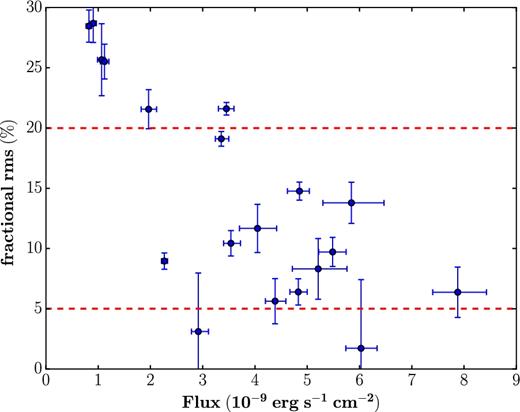
The flux in the 0.6–10 keV band versus the fractional rms. The red lines represent the fractional rms equal to 5 per cent and 20 per cent, respectively.
4 SUMMARY AND DISCUSSION
We studied the long-term light curves of GS 1826−238 observed by MAXI and Swift/BAT. We found that this source was located in a persistent and hard state before 2014, and after that several SPs were detected. Two branches are observed in Fig. 2, which approximately correspond to the SP and the persistent state. During the persistent state, the soft X-rays are faint (below 0.2 counts s−1 detected by MAXI), while the hardness (4–10 keV/2–4 keV) and the intensity of hard X-rays (15–50 keV) are relatively large. During SPs, hard X-rays are faint (below 0.005 counts s−1 detected by BAT), and the hardness is small, but slightly increases with the increasing of the flux.
We also analysed 21 Swift/XRT observations of the GS 1826−238 with an averaged exposure time ∼2213 s. Four of them were performed in a persistent state before 2014, and others were observed during the SPs (or the state between the hard state and SPs) afterwards with different flux levels. Since no SPs were observed before 2014, the work presented here is the first study of the spectral evolution (0.6–10 keV) of GS 1826−238 during SPs. We tried to fit XRT spectra by using a single Comptonization model, i.e. ‘tbabs*nthcomp’, and in general obtained an acceptable goodness of fit. An extra model, e.g. a blackbody or another Comptonization model, is not required to describe spectra, except for three observations. Even for these three observations, the ‘tbabs*nthcomp’ model can approximately describe the spectral shape of the data. The wide-band spectrum of GS 1826−238 in the persistent state has been well studied by using many satellites, e.g. INTEGRAL, BeppoSAX, RXTE + Chandra, Suzaku and NuSTAR (Thompson et al. 2005, 2008; Cocchi et al. 2010, 2011; Chenevez et al. 2016; Ono et al. 2016). Most of them suggest a dual Comptonization model, although the underlying physical explanations suggested are quite different. The reason why we cannot detect extra spectral components might be the following. First of all, the low statistics does not allow us distinguish the secondary Comptonization from the primary one, which dominates the spectrum; secondly, the limitation of the XRT energy range, i.e. no detection above 10 keV, which implies that the spectra might consist of multi-components, as suggested by Thompson et al. (2005), but this cannot be verified in XRT's energy range. Therefore, broad-band observations with good data quality are required to investigate the detailed broad-band spectral shape of GS 1826−238, especially during the SPs. We also tried to fit the XRT spectra by using other empirical models in LMXBs, i.e. two blackbody models (bbodyrad+bbodyrad) and disc-blackbody or blackbody + powerlaw (discbb/bbodyrad + powerlaw), and found that all of them could lead to an acceptable goodness of fit. But for the dual-blackbody model, the resulting radii of blackbodies are unphysical (∼20 and ∼3 km). In the ‘discbb/bbodyrad + powerlaw’ models, the thermal part mainly contributes to soft X-rays, while the power-law component dominates the hard X-rays. When the flux increases, the flux ratio of the two components remains constant. It is unusual for the typical outbursts in LMXBs, in which the thermal component will gradually dominate the whole spectrum and the power-law component will be suppressed with the increasing of the flux (Remillard & McClintock 2006; Muñoz-Darias et al. 2014). Actually, the ‘discbb/bbodyrad + powerlaw’ models are quite similar to the ‘nthcomp’ model that we used above, because the thermal parts correspond to the seed photons that suffer from unsaturated Compton scatterings, and the power-law component can describe the Compton scattering phenomenologically (except for low- and high-energy rollovers).
We find that during SPs, both the hydrogen column density (NH) and the temperature of the seed photons (Tbb) are variable. However, we note that the NH and Tbb parameters are strongly degenerate [see the inset of fig. 6 in Thompson et al. (2008)], and both of them can be significantly influenced by the selection of spectral models that cannot be disentangled by using XRT data. If we freeze NH at a given value, for example, 0.3 × 1022 cm−2, the goodness of fit will be unacceptable (the null hypothesis probability <0.01) for 10 out of 21 observations. For these observations, clear residuals appear at soft X-rays (≲2–3 keV). In this case, the photon index is only changed slightly, while the seed photon temperature (Tbb) will be influenced significantly because of its degeneracy with NH. For the frozen NH, the Tbb is ∼0.3–0.6 keV and shows no correlation with the flux. The origin of the NH variability is unknown. We speculate that it might derive from the presence of an additional component at very soft X-rays, which cannot be detected by XRT. The asymptotic power-law photon index (Γ), instead, is a phenomenological parameter, which is independent of the selected model. We confirmed that the XRT spectra in the 3–10 keV range could be fitted successfully by using a simple power-law model, and the inferred index (Γpow) is well consistent with Γ reported in Table 1. We find that the Γ is correlated with the flux (F5) when F < 2-3 × 10− 9 erg s− 1 cm− 2, and is anti-correlated with F at a higher flux level. We estimated the bolometric flux (Fbol, extended to the 0.1–100 keV band). We tried several values, i.e. 20, 10 and 5 keV, for Te parameter that cannot be constrained by using XRT data. We found that during the SPs Fbol is generally larger than F only by a factor of ∼1.5, which is smaller than the F variability of ∼3 during SPs. Therefore, we could also approximately expect an anti-correlation between Γ and Fbol in the SPs. In the hard persistent state, Fbol is larger than F by a factor of ∼3–4. Then the Fbol in the hard state should be smaller than that in the peaks of the SPs, but might be comparable with the Fbol in the relative faint state of SPs. So the relationship between Γ and Fbol during the transition to the SP is unknown. Assuming a distance of 5.7 kpc (Chenevez et al. 2016) and an isotropic radiation, the critical flux corresponds to a critical luminosity (Lcir) of 6 per cent–9 per cent |$\frac{{\rm M}_{{\odot }}}{M}$|LEdd, where M and LEdd = 1.3 × 1038 erg s−1 represent the mass of the NS and the Eddington luminosity, respectively. The relationship between Γ and the luminosity (L) in XRBs was studied by Wu & Gu (2008). They found that Γ and L are positively (negatively) correlated when L is larger (smaller) than ∼1 per cent Ledd. Our result is only consistent with Wu & Gu (2008) when L < Lcir. When L > Lcir, however, the situation is rather different. We also studied the variability of XRT observations based on the fractional rms, which is a very helpful probe to investigate the source properties. The fractional rms is ∼25 per cent during the persistent state and falls within 5 per cent and 20 per cent during SPs. The detailed properties of the variability in XRBs were reported by Muñoz-Darias et al. (2011, 2014). They found that the fractional rms is a good tracer of accretion regimes. In general, the fractional rms is ≳20 per cent in the hard state, in which the spectrum is dominated by a power-law component, and ≲5 per cent in the soft state, in which the spectrum is dominated by a thermal component. The state between these two canonical states can be regarded as an intermediate state. Therefore, observations of GS 1826−238 during the persistent state are clearly located in the hard state, which is fully consistent with previous conclusions. The observations during SPs should be classified as the intermediate state in the atoll source, which is in agreement with their spectral properties, i.e. no thermal components are detected. As shown in Fig. 1, some XRT observations were taken close to the peaks of SPs. This means that it is likely that GS 1826−238 never entered into the soft state. Here we note that we cannot study the spectral evolution along with one SP since the XRT observations were observed in different SP circles. However, the smooth evolution of the Γ suggests a hint that this source is not a typical ‘atoll’ source. Instead, it seems that the source could evolve into a bright atoll or a Z branch during SPs (for details, see fig. 9 in Muñoz-Darias et al. 2014).
Acknowledgements
JL thanks support from the Chinese NSFC 11733009. ZS thanks support from XTP project XDA 04060604, the Strategic Priority Research Programme ‘The Emergence of Cosmological Structures’ of the Chinese Academy of Sciences, Grant No. XDB09000000, the National Key Research and Development Programme of China (2016YFA0400800) and the Chinese NSFC 11473027 and 11733009. VFS thanks support from the German Research Foundation (DFG) grant WE 1312/51-1 and the Russian Government Program of Competitive Growth of Kazan Federal University. LD acknowledges support by the Bundesministerium für Wirtschaft und Technologie and the Deutsches Zentrum für Luft und Raumfahrt through the grant FKZ 50 OG 1602.
1 Crab = 3.3 counts cm− 2 s− 1, see http://134.160.243.77/star_data/J0534+220/J0534+220.html.
The null hypothesis probability, which is the probability of the observed data being drawn from the model, is calculated analytically based on the χ2-distribution shown in Table 1.
Here the flux (F) is estimated in the energy range of 0.6–10 keV.
REFERENCES
