


Abstract
Annihilating dark matter (DM) models offer promising avenues for future DM detection, in particular via modification of astrophysical signals. However, when modelling such potential signals at high redshift, the emergence of both DM and baryonic structure, as well as the complexities of the energy transfer process, needs to be taken into account. In the following paper, we present a detailed energy deposition code and use this to examine the energy transfer efficiency of annihilating DM at high redshift, including the effects on baryonic structure. We employ the pythia code to model neutralino-like DM candidates and their subsequent annihilation products for a range of masses and annihilation channels. We also compare different density profiles and mass–concentration relations for 105–107 M⊙ haloes at redshifts 20 and 40. For these DM halo and particle models, we show radially dependent ionization and heating curves and compare the deposited energy to the haloes’ gravitational binding energy. We use the ‘filtered’ annihilation spectra escaping the halo to calculate the heating of the circumgalactic medium and show that the mass of the minimal star-forming object is increased by a factor of 2–3 at redshift 20 and 4–5 at redshift 40 for some DM models.
1 INTRODUCTION
The potential impact of annihilating and decaying dark matter (DM) in the context of standard astrophysics has shown itself to be a promising avenue in the exploration of DM phenomenology (Chen & Kamionkowski 2004; Padmanabhan & Finkbeiner 2005; Furlanetto, Oh & Pierpaoli 2006; Slatyer 2013; Valdés et al. 2013; Bertone & Hooper 2016). This is in part because annihilating models are well motivated from a particle physics perspective, often arising naturally within new theoretical frameworks for physics beyond the standard model (Bertone, Hooper & Silk 2005; Bergstrom 2012; Roos 2012), but also because their non-gravitational interactions make them attractive candidates for possible future detection.
Indirect searches for annihilating and decaying DM focus on the detection of the highly energetic annihilation products that maybe used to infer the existence of the parent particles. As any non-gravitational interaction such as annihilation is assumed to be at or around the weak scale, in general a high-density region, such as found at the centre of Milky Way, is required for detectable particle excesses (Prada et al. 2004; Grasso et al. 2009; Cohen et al. 2012).
While the Galactic Centre presents a relatively accessible overdense region of DM, it is also home of one of the most astrophysically rich regions in the Milky Way. This highlights an ongoing complication with these kinds of experiments as they rely on meticulous treatment of the underlying astrophysics in order to disentangle a potential DM signal. More often that underlying physics is not yet fully understood or the signal may even be degenerate with a standard process. Similarly, uncertainty in the underlying DM structure (Mack 2014) makes for further complications, though non-detections from dwarf spheroidal galaxies occupying the Milky Way's subhaloes have been used to constrain the annihilation cross-section for some DM models.
Instead of focusing on a single, dense, and sufficiently near region of DM to detect an excess in the associated annihilation products, another possibility is to look for the potential global impact DM annihilation may have on standard cosmic evolution. One of the most exciting is the potential modification of the 21 cm signal associated with the epoch of reionzation. There are a number of ways in which the additional injected energy from DM annihilation and decay could produce changes including direct heating and ionization of the intergalactic medium (IGM; Evoli, Mesinger & Ferrara 2014; Poulin, Serpico & Lesgourgues 2015; Lopez-Honorez et al. 2016) as well as secondary effects from DM modification of baryonic structure. A number of next-generation radio telescopes such as the Square Kilometre Array (Mellema et al. 2013), Precision Array for Probing the Epoch of Reionization (Pober et al. 2013), and the Low-Frequency Array (Chapman et al. 2012) are preparing to probe the epoch of reionization using the 21 cm signal (Mesinger, Ewall-Wice & Hewitt 2014).
The following work is motivated by the prospect of using global signals such as the 21 cm line of neutral hydrogen or other observables such as galaxy properties to constrain annihilating DM models. One of the pivotal aspects of this is the integration of DM annihilation with standard astrophysical processes, such as star formation and the heating of the IGM, as well as potential complex feedback mechanisms between forming structure and the injected annihilation products. The impact of DM annihilation on individual haloes has previously been discussed in Mapelli & Ripamonti (2007), Spolyar, Freese & Gondolo (2008), Natarajan, Tan & O'Shea (2009), Gondolo et al. (2013) as well as our previous work (Schön et al. 2015, , from here on S15).
In S15, we performed a first-order calculation to gauge the impact of DM annihilation on early structure formation. We employed a simplified energy transfer process based on the medeaii code (Evoli et al. 2012) to cover a wide parameter space and a range of DM halo and particle models. We showed that in small, high-redshift objects, the energy input from DM annihilation over the Hubble time is comparable to the gravitational binding energy of the object. In this paper, we foremost look to update the energy transfer code used in S15 to allow the full evolution of the injected annihilation products, including the secondary particle cascades. The new version of the code also determines the radial distribution of the deposited energy in and outside the halo.
To demonstrate the use of the code, we revisited the halo parameter space from our previous work. This paper is structured in the following manner: Sections 2 and 3 outline the DM halo and particle models employed throughout the work and Section 4 introduces the Monte Carlo code used to calculate the energy transfer in and around the chosen haloes. The ionization and heating curves are calculated, showing the radial distribution of deposited energy within the halo and presented in Section 5 along with the comparison to the haloes’ gravitational binding energy. Section 6 shows how the initial injection spectra of the different annihilation models are changed by the gas component of the halo and how the energy that escapes into the circumgalactic medium (CGM) can heat the surrounding gas sufficiently to increase the mass of the minimal baryonic object for some haloes. The paper concludes with a discussion in Section 7 of results.
Throughout the paper, we take the cosmological parameters to be in keeping with the Planck Collaboration XIII (2016) so that h = 0.71, ΩΛ, 0 = 0.6825, Ωb, 0h2 = 0.022 068, and Ωdm, 0h2 = 0.120 29.
2 DM MODEL
We employ the same effective, self-annihilating, neutralino-like DM particle model as in S15, albeit with an additional 130 MeV, 10 GeV, and 100 GeV particle annihilating directly to an electron/positron pair. A natural choice of cross-section is close to that of the weak interaction as this gives the correct current-day density if DM is assumed to be a thermal relic. In this work, it is assumed that DM is cold and the velocity-averaged annihilation cross-section is taken as constant, regardless of environment. We set the annihilation cross-section for the 130 MeV model annihilating to an electron/positron pair to be 1.0 × 10⁻²⁸ cm−3 s−1 to be in keeping with the latest DM annihilation limits from cosmic microwave background (CMB) measurements (Madhavacheril, Sehgal & Slatyer 2014; Planck Collaboration XIII 2016). The cross-section for all other mass models is adjusted so that the total annihilation power is the same as that of the 130 MeV model to allow for comparison of the energy transfer efficiency of DM models with different masses and annihilation channels.
2.0.1 Annihilation power
2.0.2 Annihilation channels
We consider annihilation via muons, quarks, tau lepton, and W bosons as well as annihilation straight to electron–positron pairs. To implement this, an electron and a positron are collided to produce the immediate annihilation product, where the centre of mass energy of the e− and e+ is used as a proxy for the DM candidate mass. In the case of unstable annihilation products, the particles were further evolved in pythia (Sjostrand, Mrenna & Skands 2006, 2008) until only stable particles remain (see appendix A of S15 for detailed final electron, positron, and photon energy distributions). The different DM annihilation models are summarized in Table 1.
Summary of the different DM annihilation models considered in this paper.
| DM | mdm | Annihilation | Cross-section |
|---|---|---|---|
| model | (GeV) | channel | (|$\mathrm{cm^{3}\, \mathrm{s^{-1}}}$|) |
| DM1 | 0.13–100 | e− | 10−28 to 7.7 × 10⁻²⁶ |
| DM2 | 5, 20, 50 | τ | 3.8 × 10⁻²⁷, 1.5 × 10⁻²⁶, 3.8 × 10⁻²⁶ |
| DM3 | 5, 20, 50 | μ | 3.8 × 10⁻²⁷, 1.5 × 10⁻²⁶, 3.8 × 10⁻²⁶ |
| DM4 | 5.5, 20, 50 | q | 4.2 × 10⁻²⁷, 1.5 × 10⁻²⁶, 3.8 × 10⁻²⁶ |
| DM5 | 83, 110 | W | 6.4 × 10⁻²⁶, 8.5 × 10⁻²⁶ |
The annihilation process can also produce a significant fraction of neutrinos. However, as these only interact on the weak scale with the surrounding gas, we assume that they do not contribute in a significant fashion to the energy transfer process and we thus do not consider them further in this work.
3 HALO MODELS
In order to investigate the degree to which DM annihilation transfers energy into the halo and CGM, we require models for the DM and gas distribution within the halo as well as a density profile for the gas immediately surrounding the halo. We note that since we are primarily interested in high-redshift haloes with masses well below the general resolution limit of N-body simulations, there is a considerable degree of uncertainty involved in these models (Mack 2014).
3.1 DM density profiles
3.1.1 Mass–concentration relation
The mass–concentration parameter c is a free parameter of the profiles described above, which sets the turn-over of the density gradient. It is of particular interest in DM annihilation calculations because it can significantly enhance the overall power output in individual haloes by increasing the DM density at its core.
The concentration parameter is well described (Comerford & Natarajan 2007; Duffy et al. 2008; Ludlow et al. 2013) for galaxy hosting haloes at low redshifts. However, simply extrapolating these mass–concentration relations to the required masses and redshifts can lead to haloes with extremely dense cores, which in turn could potentially overestimate the DM annihilation signal. The evolution of the mass–concentration parameter for the small masses and high redshifts reviewed in this work is less well constrained (Prada et al. 2012; Dutton & Macciò 2014; van den Bosch et al. 2014; Diemer & Kravtsov 2015). The determination of the behaviour for low-mass haloes in particular is restricted by the mass resolution of N-body simulations. In addition to mass resolution, different equilibrium cuts (Neto et al. 2007) imposed on the respective halo samples could be a further factor contributing to the discrepancies found between the mass–concentration relations cited above. The impact of these unsettled haloes on the mass–concentration relation becomes more pronounced at high redshift where a large fraction of the halo population is not in a relaxed state due to elevated merger rates.
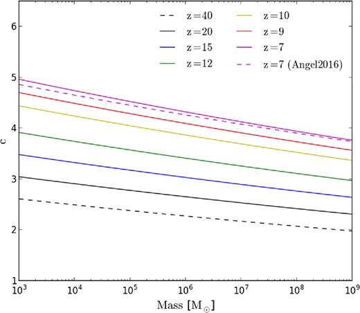
The fiducial mass–concentration relation used in this work. Solid lines show the semi-analytic model from Correa et al. (2015) at various redshifts with the dashed black curve showing an extrapolation to redshift 40. The dashed pink line shows results from Angel et al. (2016) that were extracted from N-body simulations.
Lastly, we summarize the different halo models in Table 2. Throughout the paper, the ‘fiducial’ and ‘Burkert’ models refer to haloes with the Correa mass–concentration relation and an Einasto and Burkert density profile, respectively. The ‘high’ and ‘Burkert-high’ models refer to haloes with Einasto and Burkert profiles as well as an increased c parameter, here taken to be double that of the Correa model. The highly concentrated model was chosen to account for the uncertainty in the mass–concentration relation, as well as natural scatter found in the relevant halo population (Angel et al. 2016).
Summary of the different DM halo models considered in this work.
| Halo model | Mass | Redshift | c | Profile |
|---|---|---|---|---|
| log10[M⊙] | (z) | |||
| Fiducial | 5–7 | 20, 40 | Correa | Einasto |
| Burkert | 5–7 | 20, 40 | Correa | Burkert |
| High | 5–7 | 20, 40 | Correa × 2 | Einasto |
| Burkert-high | 5–7 | 20, 40 | Correa × 2 | Burkert |
| Halo model | Mass | Redshift | c | Profile |
|---|---|---|---|---|
| log10[M⊙] | (z) | |||
| Fiducial | 5–7 | 20, 40 | Correa | Einasto |
| Burkert | 5–7 | 20, 40 | Correa | Burkert |
| High | 5–7 | 20, 40 | Correa × 2 | Einasto |
| Burkert-high | 5–7 | 20, 40 | Correa × 2 | Burkert |
3.1.2 Dynamic haloes
At this point, a brief mention should be made about the assumption that the haloes under consideration here are in a static state of equilibrium, and that both the underlying DM structure and the baryonic content of the halo remain unchanged. More realistically, haloes after collapse will grow through a combination of merger events and inflowing gas. At high redshifts especially, the rapid merger rate means that a significant fraction of haloes are not relaxed, and moreover, recovery takes place over a number of dynamical times (Poole et al. 2016).
The disruption of both the DM and gas density distributions associated with mergers could subsequently impact both the DM annihilation power and the absorption efficiency. In addition, self-consistent modelling of the halo incorporating the potential ongoing effects due to the halo self-heating, such as expulsion of gas, is not accounted for. These concerns are anticipated to be included in future work.
3.2 Gas model
3.2.1 Baryonic density distribution within the halo
3.2.2 Circumgalactic density distribution
4 ENERGY TRANSFER CODE
We update the energy transfer code used in S15 to more fully model the paths of the injected particles (as well as the secondary particles created in the subsequent cascades) throughout the halo. In addition, the updated code allows us to record the spatial distribution of the deposited energy in the form of heating, ionization, and Lyman photons as well as keep a record of the energy distribution of the particles that escape the halo.
4.1 Processes
In our treatment of the relevant interaction processes, we closely follow the treatment of Evoli et al. (2012) and Slatyer, Padmanabhan & Finkbeiner (2009).
4.1.1 Electrons and positrons
At high energies, electrons and positrons predominantly lose energy through inverse Compton (IC) scattering off CMB photons (Blumenthal & Gould 1970) while lower energy electrons undergo collisional interaction with the gas atoms. These collisions lead to ionization (Arnaud & Rothenflug 1985; Shah, Elliott & Gilbody 1987; Shah et al. 1988; Kim & Rudd 1994), atomic excitation (Bransden & Noble 1976; Fisher et al. 1997; Stone, Kim & Desclaux 2002; Hirata 2006; Chuzhoy & Shapiro 2007), and Coulomb scattering (Spitzer & Scott 1969; Shull & Steenberg 1985; Furlanetto & Stoever 2010). Recombination (Karzas & Latter 1961) is also included, though subdominant compared to the other processes.
At high energies, positrons behave in the same manner as electrons. At low energies, they also undergo collisional interactions in addition to forming positronium via charge exchange (Heitler 1954; Guessoum, Jean & Gillard 2005).
4.1.2 Photons
In a similar fashion, photons photoionize the surrounding gas (Verner et al. 1996), Compton scatter off free electrons (Heitler 1954; Chen & Kamionkowski 2004), and at high enough energies undergo electron–positron pair production (PP). We here distinguish the cross-section for PP off of the CMB (Agaronyan, Atoyan & Nagapetyan 1987; Ferrigno, Blasi & De Marco 2005), atomic and ionized hydrogen and helium, as well as free electrons (Joseph & Rohrlich 1958; Motz, Olsen & Koch 1969; Zdziarski & Svensson 1989). Photons also undergo photon–photon scattering where the injected photon transfers part of its energy to a CMB photon (Svensson & Zdziarski 1990); however, this process is highly subdominant in the redshift range considered here.
The mean free paths (mfp) at mean gas density for selected processes undergone by injected electrons, positrons, and photons are outlined in Fig. 2 for a neutral 107 M⊙ halo at redshift 40. Solid and dot–dashed lines show interactions for the leptons while the dashed show those for photons. The dashed red, magenta, and orange lines show photoionization, Compton scattering, and pair creation off of the gas field, respectively. Electroionization and excitation are shown in green and blue, IC scattering in black, and annihilation via positronium for positron in purple. For a fully ionized halo, the yellow line shows the mfp for Coulomb interaction. For each process, the lines indicate the mfp at the average density of the halo while the shading either side of the curves shows the mfp at rvir and rvir/100.
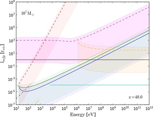
mfpin units of the virial radius for the various interactions undergone by injected particles within a neutral gas 107 M⊙ halo at redshift 40. Solid lines show interactions for charged particles and dashed for photons. The grey line indicates the virial radius of the halo. Processes shown are photoionization (red), Compton scattering (magenta), and pair creation off of the gas (orange) for photons and ionization and excitation (green and blue) for electrons, as well as IC scattering (cyan) and annihilation via positronium for positrons (purple, dot–dashed line). In all cases, lines show the mfp for the process at the average density of the halo, while the shaded regions either side indicate the mfp at rvir and rvir/100. For reference, the yellow curve shows the mfp for Coulomb scattering in an equivalent, fully ionized halo.
The grey line is indicative of the halo's virial radius. Particles with energies such that their interaction mfp are no longer smaller than or comparable to the virial radius will readily escape the halo without either interacting with the gas and/or depositing energy. For the DM annihilation products considered here, the primary interaction of the injected electrons and positrons is IC scattering (injected photons first undergo electron/positron pair creation off of the gas field). The actual energy transfer process occurs via the secondary particle produced in those interactions, in this case, the upscattered IC photons. Therefore, the energy spectrum of the secondary cascade products induced by the injected particles plays an important role in determining the relative efficiency with which the different DM models are able to deposit energy into the halo.
4.2 Particle evolution
The step-wise evolution of the particle follows the methodology of the GEANT4 simulation toolkit (Agostinelli et al. 2003; Allison et al. 2006). At the beginning of each calculation, the code takes a particle (in this case, an electron, photon, or positron) with a given energy and injects it at point |$\boldsymbol {x}$| in direction (θ, ϕ). The particle then takes a straight line step of size determined by the step-size function in this specified direction. The code then selects a random point along this straight line step and uses the densities at this point to calculate the relevant mfp that characterize the distance the particle travels before said interactions take place. For each potential process, random numbers are used to determine at what point the interaction takes place. If none of the interactions take place within the step size, the particle travels to the end of the straight line, the next step is taken, and the process is repeated. If one or more interactions do occur within the step, the process corresponding to the shortest distance to interaction will be executed. At the end of the process, the code records the location of any energy that has been deposited as well as the type, energy, position, and orientation of the remaining/newly created particles. The process repeats until either all particles’ energies drop below all interaction thresholds (or if one is defined, the particle escapes a pre-defined spatial boundary).
The initial particle can be evolved as often as required to achieve the necessary level of convergence. At the end of the Monte Carlo run, the code outputs the average energy deposited into heating, ionization, and Lyman α photons in each pre-defined spatial bin as a fraction of the original injected particle's energy. If a physical boundary is defined, the code will give a similarly normalized spectrum of the escaped electrons, positrons, and photons.
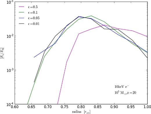
Outputs for a 10 keV electron injected into 105 M⊙ halo at redshift 20 for different step-size scale parameters ε. Magenta, green, blue, and black curves, respectively, refer to ε = 0.5, 0.1, 0.05, and 0.01. Results are given as the fraction of the original injected particle energy deposited in each respective radial bin.
5 HALO SELF-HEATING
We now use the code to calculate the energy deposited within 105, 106, and 107 M⊙ haloes at redshifts 20 and 40.
5.1 Heating and ionization
Fig. 4 shows selected heating and ionization curves for different halo and DM particle models. All results are given as the fraction of the total annihilation power of the halo deposited per unit volume. Upper plots show the outputs for a 105 M⊙ halo at redshift 20. The figure on the left shows a 5 GeV particle annihilating via tau leptons (magenta) and quarks (cyan) while the figure on the right shows models annihilating via muons with 5, 20, and 50 GeV shown in blue, green, and yellow. In both plots, the black curves show the 130 MeV model annihilating directly to an electron/positron pair with the solid, dashed, and dotted lines showing energy going into heating, ionization, and Lyman photons for reference.
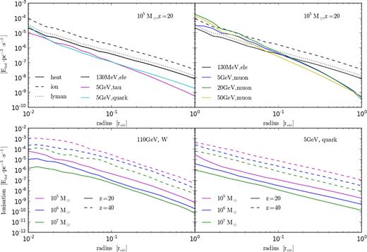
Heating and ionization curves for different haloes and DM models. All results are given as the fraction of the total annihilation power of the halo deposited per unit volume. Upper plots show the outputs for a 105 M⊙ halo at redshift 20. The figure on the left shows a 5 GeV particle annihilating via tau leptons (magenta) and quarks (cyan) while the figure on the right shows models annihilating via muons with 5, 20, and 50 GeV shown in blue, green, and yellow. In both plots, the black curves show the 130 MeV model annihilating directly to an electron/positron pair with the solid, dashed, and dotted lines showing energy going into heating, ionization, and Lyman photons for reference. The lower-left plot shows results for a 110 GeV DM particle annihilating via W bosons and the lower right shows those for a 5 GeV particle annihilating via quarks, In each of the lower plots, magenta, blue, and green curves show the ionization curves for 105, 106, and 107 M⊙ haloes where solid lines indicate outputs at redshift 20 and dashed those at redshift 40.
As mentioned previously, the relative energy transfer efficiency of the various DM models is strongly dependent on the energy distribution of the secondary cascade particles. Of particular note is the 130 MeV model annihilating via an electron/positron pair shown in black in the upper row of Fig. 4. Electrons/positrons injected at 130 MeV will produce upscattered IC photons with energies low enough to undergo photoionization so that even the lower density regions at the edge of the halo can be heated. This, along with the fact that none of the annihilation power is lost to neutrinos, makes it a very attractive DM candidate as far as possible detection goes.
For somewhat heavier DM models (1–5 GeV), the peak of upscattered IC photons will fall into the energy regime of Compton scattering, which is only efficient at the high gas densities found at the centre of the halo. Even heavier candidates will eventually produce IC photons sufficiently energetic to undergo pair creation themselves leading to more complex cascades. In both of those scenarios, the energy deposition in the outer parts of the haloes is less efficient due to a significant fraction of the resultant cascade particles falling into energy regimes in which interaction with the gas is poor. Lastly for neutral gas, the majority of the deposited energy is partitioned into ionization as is indicated by the black dashed line in the upper plots of Fig. 4. However, as the halo becomes ionized, Coulomb heating very rapidly becomes a dominant interaction process and the energy partition becomes skewed towards heating instead.
The lower-left plot shows results for a 110 GeV DM particle annihilating via W bosons and the lower right shows those for a 5 GeV particle annihilating via quarks, In each of the lower plots, magenta, blue, and green curves show the ionization curves for 105, 106, and 107 M⊙ haloes where solid lines indicate outputs at redshift 20 and dashed those at redshift 40. As expected, the energy deposition efficiency at higher redshifts is greater due to the increase in both the gas and CMB number density.
5.1.1 Lyman photons
As shown in Fig. 4, our code also tracks the production of Lyman photons. Photons with energy below the Lyman limit (13.6 eV) are assumed to cease direct interaction with their surrounding medium. However, their production through DM annihilation can still play an important role in baryonic structure formation when taking gas cooling into account. For instance, photons with energies between 11.2 and 13.6 eV are classified as Lyman–Werner photons. These photons maybe absorbed by molecular hydrogen and through excitation and subsequent radiative decay lead to its disassociation. Before the production of metals, the formation and destruction of H2 play an important role in molecular cooling at high redshifts (Abel et al. 1997) and are thus vital for early star (Abel, Bryan & Norman 2002) and galaxy formation (Bromm et al. 2009). For the calculation performed here, all photons with energy between 10.2 and 13.6 eV were counted towards the Lyman photon output. Those with energy below 10.2 eV were taken to no longer interact with the halo's gas component and discarded.
5.2 Binding energy comparison
Fig. 5 shows the comparison Rg between the energy deposited over the Hubble time and the gravitational binding energy of the haloes at different radii. For a 106 M⊙ halo at redshift 20, the upper plots compare different halo models where the solid, dotted, dashed, and dot–dashed lines show the results for the fiducial, Burkert, high, and Burkert-high models, respectively. As previously discussed, models with more concentrated mass profiles both produce more annihilation power and are more efficient at depositing energy into the halo. This can be seen here when comparing the high model to the others. Also of interest is that the Burkert-high model is, with exception of the behaviour very close to the halo centre, nigh indistinguishable from the fiducial model. In this scenario, doubling the mass–concentration parameter allows the flat-core Burkert profile to mimic the behaviour of the cuspy Einasto profile, again highlighting the potential impact underlying uncertainties in the DM models have on results. The lower plot shows results for different annihilation channels where black, blue, and green show the tau lepton, muon, and quark models.
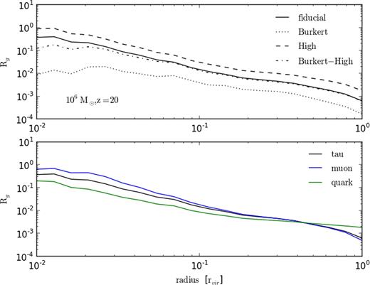
The ratio Rg comparing the energy deposited as heat over the Hubble time with the gravitational binding energy of shells at different radii in a 106 M⊙ halo at redshift 20. The upper plot compares different DM haloes models for a 20 GeV DM particle annihilating via tau leptons. The fiducial halo model is shown by the solid black line and the Burkert model is shown by the dotted curve. The high and Burkert-high models are given by the dashed and dot–dashed curves, respectively. The lower plot shows Rg for the fiducial halo model but with the black, blue, and green lines showing models annihilating via tau leptons, muons, and quarks.
Fig. 6 also shows Rg but here haloes at different redshifts are compared. From left to right, the plots show results for 130 MeV particle annihilating to an electron/positron pair, 20 GeV annihilating to quarks, and 110 GeV annihilation to a W boson. As before, magenta, blue, and green curves correspond to 105, 106, and 107 M⊙ haloes while solid lines refer to results at redshift 20 and dashed to those at redshift 40. Also as before, Rg is greater at high redshift due to the higher energy transfer efficiency. The sustained heating of the 130 MeV model out to the edges of the halo is also demonstrated again.
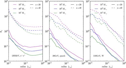
The ratio Rg of heating from DM annihilation over the Hubble time and gravitational binding energy at different radii. From left to right, the plots show results for 130 MeV particle annihilating to an electron/positron pair, 20 GeV annihilating to quarks, and 110 GeV annihilation to a W boson. As before, magenta, blue, and green curves correspond to 105, 106, and 107 M⊙ haloes while solid lines refer to results at redshift 20 and dashed to those at redshift 40.
As a whole, this matches the findings of the work in S15, albeit with a more precise estimate of the deposition fractions. Having an additional, not insignificant heating source during the early stages of these micro-haloes’ development could result in gas being expelled, or alternatively heated to a degree that prevents/delays star formation. A dynamic model would be required to ascertain how impactful the heating from DM turns out to be. While this is beyond the scope of this work, the heating curves calculated here are an important first step towards fully quantifying the impact DM annihilation has on early star formation.
6 HEATING OF THE CGM
While it was here shown that energy comparable to that of the binding energy is deposited inside the halo over the Hubble time, most of the injected energy will escape the halo. In this section, the results from this calculation are used to determine the changes to the particle distribution of the original annihilation spectrum as a consequence of traversing the halo. These new spectra are then injected into the CGM to establish whether there is sufficient heating to curtail the infall of gas on to the halo, and therefore affect structure formation.
6.1 Filtered spectra
Fig. 7 demonstrates the code output showing the energy distribution of particles escaping a 106 M⊙ halo at redshift 20. The uppermost plot shows the distribution of escaped electrons (left), photons (middle), and positrons (right) for 5 GeV electrons injected into the halo. The plots directly below show the same but for a 5 GeV photon. The lower two plots show the total spectrum where the third row shows the original, unmodified injected annihilating spectrum for a 5 GeV DM particle annihilating via muons. The lowest plot shows the spectra after the injected particles have passed through the halo. In both plots, the pink columns show photons, blue electron, and green positrons, and results are given as a fraction of the halo's total annihilation power.
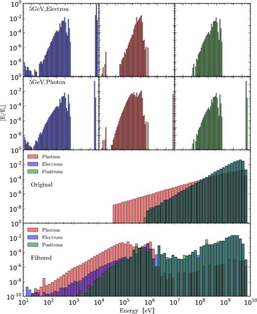
Code output showing the energy distribution of particles escaping a 106 M⊙ halo at redshift 20. The uppermost plot shows the distribution of escaped electrons (left), photons (middle), and positrons (right) for 5 GeV electrons injected into the halo. The plots directly below show the same but for a 5 GeV photon. The lower two plots show the total spectrum where the third row shows the original, unmodified injected annihilating spectrum for a 5 GeV DM particle annihilating via muons. The lowest plot shows the spectrum after the injected particles have passed through the halo. In both plots, the pink columns show photons, blue electron, and green positrons, and results are given as a fraction of the halo's total annihilation power.
As can be seen in the modified spectra, the original electron/positron distribution is largely retained as only a small fraction of energy is actually lost to the halo, though it is somewhat broadened towards lower energies. In contrast, the original high-energy photons undergo pair creation and only those photons injected close to the virial radius are retained. The secondary population of pair-created electrons and positrons can be observed around 104–106 eV. Electrons also feature a low-energy tail due to ionization from those IC photons that fall below the pair-creation limit. IC scattering will create an extensive secondary population of photons with those IC photons below the pair-creation limit comprising the prominent mid- to low-energy tail.
While we focus here on the impact on a halo's immediate environment, this modification of the spectrum also has implications for the impact of annihilation products on the mean IGM evolution. The efficiency of energy deposition depends strongly on the energy spectrum of the photons and particles, suggesting that the filtering must be taken into account in studies of DM's impact on reionization.
6.2 Raising Jeans mass
Figs 8 and 9 show the modified δb from DM annihilation for a 105 M⊙ halo at redshifts 20 and 40. Different colours correspond to different DM annihilating channels with blue, red, green, magenta, and black showing the electron/positron, muon, quark, tau, and W boson channels, respectively. Different symbols as indicated in the bottom-left plot indicate different DM masses. From left to right, the top plots show the fiducial and high halo models and the lower show results for Burkert and Burkert-high models.
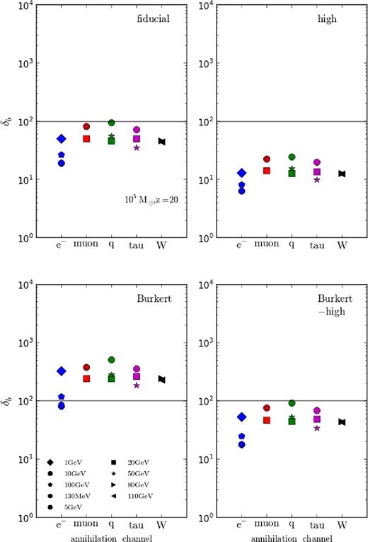
Modification of δb from DM annihilation for a 105 M⊙ halo at redshift 20. Different colours correspond to different DM annihilating channels with blue, red, green, magenta, and black showing the electron/positron, muon, quark, tau, and W boson channels, respectively. Different symbols as indicated in the bottom-left plot indicate different DM masses. From left to right, the top plots show the fiducial and high halo models and the lower show results for Burkert and Burkert-high models. The grey horizontal line shows the critical δb chosen to indicate the minimal δb required for baryonic collapse.
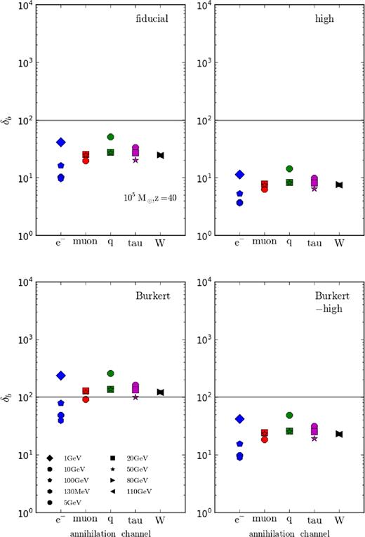
The results for the 105 M⊙ haloes in Figs 8 and 9 suggest that for a number of DM particle and halo models, the additional heating from DM annihilation will lower δb below 100. As expected, this effect is most pronounced for the highly concentrated Einasto-high halo model due to the increase in annihilation power. In comparison, results for the standard Burkert model show the impact to be reduced by about an order of magnitude. Understandably, the fiducial model falls between the two extremes with the concentrated Burkert profile again producing results comparable to that of the fiducial model.
In terms of DM particles, the 130 MeV model annihilating to an electron/positron pair is the most effective in reducing δb due to both its efficiency in depositing energy into the gas locally and the fact that none of the annihilation energy is siphoned into neutrinos. Amongst the remaining annihilation channels, heavier candidates provide a greater change in δb compared to models with masses from 1to5 GeV. This is in keeping with the previous discussion that showed that electrons and positrons within that energy range produce IC photons that tend to free stream at IGM densities. Results for the halo at redshift 40 are qualitatively similar to those at redshift 20 but with δb reduced even further.
While not shown here, results indicate that δb is not significantly impacted for the 106 and 107 M⊙ haloes, though again the results are comparable to the lower mass cases in their general behaviour. However, as was briefly alluded to earlier, the method of calculating δb does not take into account the virialization shocks surrounding the haloes and for 107 M⊙ haloes shock heating of the surrounding gas becomes significant. The derivation of δmod in equation (16) however assumes that the gas temperature remains at the temperature of the IGM, and therefore the method does not produce reliable results for haloes of this mass.
6.3 Change in the minimal baryonic mass
If δb is sufficiently reduced due to DM annihilation in 105 M⊙ haloes at redshifts 20 and 40, what consequences does this suggest for the minimal baryonic objects? Fig. 10 again shows the annihilation-modified δb though this time as a function of halo mass. The top panel shows the results at redshift 20 and the lower panel at redshift 40. In both plots, the grey, horizontal line denotes δb = 100, which gives the chosen critical value for the collapse of baryonic structures. Different coloured curves show the outputs for different halo/DM models.
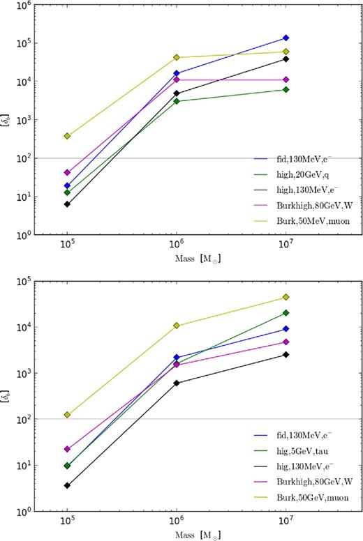
Modification of δb from DM annihilation for different halo masses and DM models. The grey horizontal line again shows the critical δb chosen to indicate the minimum δb for sufficient gas accretion on to the halo.
For δb = 100 as the critical value, a number of DM candidates would reduce the infall of gas on to the halo to a degree that potential baryonic structure formation could be affected. For the DM model with the most pronounced impact on δb, a 130 MeV particle with a concentrated Einasto profile (black curve), a 105 M⊙ halo would have to increase in mass by a factor of 2–3 at redshift 20 and 4–5 at redshift 40 to recover a δb of 100. It is again important to note that the large δb produced for haloes with mass >106 M⊙ arise due to the non-inclusion of virialization shocks and the subsequent shock heating of the gas surrounding the haloes. The derivation of δmod in equation (21) however assumes that the CGM gas temperature remains at the temperature of the IGM (which gives rise to the large δb in Fig. 10), and therefore the method does not produce reliable results for haloes of this mass. This however does not impact the conclusions drawn for the 105 M⊙ haloes.
7 DISCUSSION
In this paper, we revisited the energy deposition from DM annihilation in small, high-redshift haloes, as well as calculating the heating of the haloes’ CGM due to DM annihilation in the halo proper. A key aspect of this work is the updated energy transfer Monte Carlo code that allows for injected electrons, positrons, and photons to interact with an arbitrary, three-dimensional number density distribution of atomic hydrogen, helium, free electrons, and CMB photons. The code calculates the fraction and location of the energy deposited into heating, ionization, and Lyman photons in a pre-defined volume such as a halo.
Overall, the broad conclusions drawn in the earlier calculation are supported in the detailed study. We find that the total annihilation power is increased for more concentrated haloes, with the total annihilation power being significantly impacted by the precise distribution of DM within the halo. We also find the existence of a parameter space in which DM annihilation could modify baryonic structure formation. In our previous paper, the choice of annihilation channel influenced outcomes predominantly through the fraction of the total annihilation power partitioned into electrons/positrons and photons, as opposed to the non-interacting neutrinos. Since the updated energy transfer method is sensitive to the energy-dependent mfp, both the DM particle mass (for an annihilation cross-section adjusted to give the same total power integrated over the halo) and choice of annihilation channel also impact the overall energy deposition by changing the energy distribution of annihilation products. The 130 MeV DM model annihilating via electron/positron pairs was particularly efficient at depositing energy with haloes due to the favourable interaction mfp of the upscattered IC photons produced by the injected particles.
We built on our detailed examination of self-heating haloes by calculating the heating of the haloes’ CGM. Sufficient increase in temperature of the CGM can lead to the suppression of gas infall on to the halo and formation of baryonic structure. δmod was calculated for the different DM models. At redshifts 20 and 40, a 105 M⊙ halo is no longer massive enough for δb > 100, instead objects more massive by a factor of 3–5 are required. An important caveat is that the method used in the work breaks down for more massive haloes as it does not take into account shock heating haloes, which results in an inflated value of δb.
The work completed here aims to contribute to the identification of the parameter space in which DM annihilation impacts early structure formation as well as developing tools to assist with the rigorous treatment of energy transfer in non-homogeneous density fields. While the analysis of a single halo cannot predict the accumulative effect DM annihilation has on hierarchical structure formation over time, it does aid in the formulation of models that will be compatible with simulations and allow for testable predictions to be made.
In order to identify a signal indicative of new physics, careful modelling is required to account for both uncertainties in the DM and astrophysical models. It is crucial that predictions whether they be of a DM-modified 21 cm signal or general galaxy properties integrate DM annihilation into the emergence of structure starting at high redshifts. A number of challenges remain before the latter can be fully realized, but the prospective comparisons to be made with future observations will provide valuable constraints to guide the ongoing quest to uncover the fundamental nature of DM.
Acknowledgements
We would like to thank Tracy Slatyer and Hongwan Liu for insightful discussions. Part of the energy transfer calculation was performed using the gSTAR national facility at Swinburne University of Technology, which is funded by Swinburne and the Australian Government's Education Investment Fund. KM is supported by the Australian Research Council Discovery Early Career Research Award. Lastly, we would like to thank the anonymous referee for their valuable comments.
REFERENCES
