


Abstract
Almost all black holes (BHs) and BH candidates in our Galaxy have been discovered as soft X-ray transients, so-called X-ray novae. X-ray novae are usually considered to arise from binary systems. Here, we propose that X-ray novae are also caused by isolated single BHs. We calculate the distribution of the accretion rate from interstellar matter to isolated BHs, and find that BHs in molecular clouds satisfy the condition of the hydrogen-ionization disc instability, which results in X-ray novae. The estimated event rate is consistent with the observed one. We also check an X-ray novae catalogue (Corral-Santana et al.) and find that 16/59 ∼ 0.27 of the observed X-ray novae are potentially powered by isolated BHs. The possible candidates include IGR J17454−2919, XTE J1908−094, and SAX J1711.6−3808. Near-infrared photometric and spectroscopic follow-ups can exclude companion stars for a BH census in our Galaxy.
1 INTRODUCTION
X-ray novae are soft X-ray transient events with ∼10 d of rapid brightening up to ∼ 1038 erg s− 1, followed by exponential decays (see Tanaka & Shibazaki 1996; Chen, Shrader & Livio 1997; Yan & Yu 2015, for reviews). X-ray novae are considered to be produced by binary systems composed of low-mass stars and compact objects, such as neutron stars or black holes (BHs), so-called a low-mass X-ray binary (LMXB) system. About 20 LMXBs have been dynamically confirmed to contain BHs through spectral observations of companion stars. Furthermore, 30–40 of X-ray novae share the same X-ray signatures with those of BH LMXB systems, but they are too faint after an outburst to conduct follow-up observations (Corral-Santana et al. 2016). Therefore, strictly speaking, it is unclear whether these X-ray novae without follow-up observations are really produced by binary systems or not.
In the standard scenario, X-ray novae are explained by the hydrogen-ionization instability of accretion discs (a kind of thermal-viscous instability, see Lasota 2001, for a review). The instability model is originally proposed as a mechanism of dwarf novae, which are optical transients caused by white dwarf binary systems (Osaki 1974; Hōshi 1979), and later applied to X-ray novae (van Paradijs & Verbunt 1984; Cannizzo, Wheeler & Ghosh 1985; Huang & Wheeler 1989; Mineshige & Wheeler 1989). When a region in a disc has low temperature for hydrogen to recombine, the negative hydrogen (H−) ions dominate the opacity. As opposed to the free–free opacity, the H− hydrogen opacity is a steep increasing function of temperature. This rapid response to the temperature change makes an S-shaped structure in the thermal equilibrium curve of the region (see Fig. 1). In the quiescent phase, the region is in the low temperature branch, whereas when the surface density reaches a critical value, the region makes a transition to a hot branch and increases the mass accretion rate. Then, the inner annulus is also heated, and the whole disc mass accretes to the central object. This is the origin of X-ray brightening.
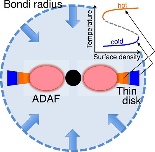
Schematic picture of an isolated BH with a thin disc part attached to inner ADAF part. The thin disc part consists of an outer cold branch and an inner hot branch in the S-shaped thermal equilibrium curve (upper right).
Recently, the advanced Laser Interferometer Gravitational Observatory (LIGO) has detected gravitational waves (GWs) and observed binary BH mergers for the first time (Abbott et al. 2016a,c, 2016d). If such merged spinning BHs exist in our Galaxy, they can be high-energy sources (Ioka et al. 2017). Before the GW detections, isolated BHs are also believed to reside in our Galaxy. Based on the stellar evolution theory, the number of isolated BHs is as many as ∼108 (Shapiro & Teukolsky 1983). Some authors have discussed high-energy phenomena caused by isolated BHs (Armitage & Natarajan 1999; Barkov, Khangulyan & Popov 2012; Teraki et al., in preparation), and studied the detectability of isolated BHs (Fujita et al. 1998; Agol & Kamionkowski 2002; Fender, Maccarone & Heywood 2013; Matsumoto & Ioka, in preparation). However, because of the very low mass accretion rate, the accretion discs around BHs are radiatively inefficient (Narayan & Yi 1994) and the detection of isolated BHs is challenging if BHs are stationary sources.
In this paper, we propose a novel idea that isolated single BHs in our Galaxy can produce transient events like X-ray novae. The structure of this paper is as follows. First, we calculate the mass accretion distribution of isolated BHs (Section 2). Next, we find that some BHs in molecular clouds accrete enough mass to have a thin disc part in Section 3. This is because for a large mass accretion rate, a disc has a high density enough to cool by radiation and become geometrically thin at the outer part of the disc (Abramowicz et al. 1995; Narayan & Yi 1995). In Fig. 1, we show a schematic picture of the system we consider. The thin disc region can suffer from the hydrogen-ionization instability and cause transient events like X-ray novae. We also estimate that the event rate is comparable to that of the observed X-ray novae. Finally, we suggest that some X-ray novae without companions could be produced by isolated BHs in Section 4. We also discuss how to discriminate an isolated BH from a binary by observations.
2 ACCRETION RATE DISTRIBUTION OF ISOLATED BHS
In this section, we consider the mass accretion on to Galactic isolated BHs. The BHs accrete interstellar medium (ISM) gas and form accretion discs. We study the accretion rate distribution of isolated BHs taking the BH mass, the BH velocity, and the ISM density distributions into account.
When magnetic fields from the ISM thread the accretion disc, the magnetic braking effect may work and reduce the disc radius. Since the efficiency of the braking effect sensitively depends on the geometry of the magnetic fields (Mouschovias 1985, and references therein), it is difficult to study whether the magnetic braking affects the disc radius. Here, we estimate the time-scale of the angular momentum transfer by the Alfvén crossing time-scale at a given radius R, and compare it with the free fall time-scale |$t_{\rm {ff}}=\sqrt{R^3/GM}$|. At the Bondi radius RB ≃ 1.3 × 1015 cm for an isolated BHs with the velocity V ≃ 10 km s− 1, each time-scale is evaluated as tA ≃ 1.0 × 10¹⁰ s and tff ≃ 1.3 × 10⁹ s for the magnetic field and the density at the Bondi radius of B ≃ 10 μG (Crutcher et al. 2010) and n ≃ 102 cm− 3. These are the typical values in molecular clouds, where isolated BHs get enough accretion rate to power X-ray novae (see below). Then, we can neglect the braking effect. At the disc radius Rd ≃ 4.8 × 1011 cm, each time-scale is estimated as tA ≃ 5.7 × 10⁵ s and tff ≃ 9.2 × 10³ s, where we use the flux freezing BR2 = const and the disc density given by equation (33). Therefore, it is unlikely that the braking effect transfers a significant amount of angular momentum, and reduces the disc radius. In order to study this effect in detail, we may need to conduct a magnetohydrodynamic simulation, but it is the beyond of the scope of this work.
For a stationary accretion disc to exist, the infall time at the Bondi radius tff(RB) should be shorter than the dynamical time of a BH to cross the Bondi radius tdyn = 2RB/v. This condition is achieved as tff(RB)/tdyn = v/2V ≃ 0.35 ≲ 1, where we set the BH velocity is equal to the sound velocity v ≃ cs.
The parameters for each ISM phase. For molecular clouds and cold |$\mathrm{H}{\, }{\small {I}{\,}}$|medium, which have broad density distributions, the minimum n1, maximum n2 number densities, and power-law index of the distributions β are shown. For the other mediums, we show the typical density in the column 2. We represent the volume filling factors ξ0, the sound velocities cs, and scaleheights Hd in column 5, 6, 7, respectively. For the sound velocity, we include the contribution of the turbulent velocity.
| Phase | n1 (cm− 3) | n2 (cm− 3) | β | ξ0 | cs (km s− 1) | Hd (kpc) |
|---|---|---|---|---|---|---|
| Molecular cloud | 102 | 105 | 2.8 | 10−3 | 10 | 0.075 |
| Cold |$\mathrm{H}{\, }{\small {I}{\,}}$| | 10 | 102 | 3.8 | 0.04 | 10 | 0.15 |
| Warm |$\mathrm{H}{\, }{\small {I}{\,}}$| | 0.3 | – | – | 0.35 | 10 | 0.5 |
| Warm |$\mathrm{H}{\, }{\small {II}{\,}}$| | 0.15 | – | – | 0.2 | 10 | 1 |
| Hot |$\mathrm{H}{\, }{\small {II}{\,}}$| | 0.002 | – | – | 0.4 | 150 | 3 |
We comment the uncertainty of the density distribution function of molecular clouds because molecular clouds are the main site where isolated BHs launch X-ray novae. The power-law distribution is obtained by the mass function of molecular clouds dNcl/dMcl ∝ Mcl−p, where Ncl and Mcl are the number of molecular clouds and the molecular cloud mass, and the density and cloud size relation (so-called Larson's third law, Larson 1981), nRcl ∝ Rclq, where Rcl is the molecular cloud size. Although the observed typical indices of p = 1.6 (Williams & McKee 1997) and q = 0 (Solomon et al. 1987) give β = 2.8, the inaccuracy of these index value may also cause an uncertainty of our result. By the observations, the indices are determined within the range of p ≃ 1.5–1.8 (Kramer et al. 1998; Rosolowsky 2005) and q ≃ 0–0.1 (Heyer et al. 2009), which result in the index β ≃ 3.0–2.4. However, this change of β increases or decreases only the maximum accretion rate (|$\dot{m}\simeq 2\times 10^{-2}$|, see Fig. 2) and does not change significantly the total number of BHs that power X-ray novae. Therefore, our main results such as the event rate do not sensitively depend on the uncertainty of the density distribution function. In addition to the density distribution, the turbulent velocity distribution may change the accretion distribution. Note that we include this contribution into the sound velocity (see the caption in Table 1). Larson's first law shows that the smaller cloud has the smaller turbulent velocity, which makes the BH accretion rate large. However, according to Larson's third law, these clouds have also large density and only change the maximum accretion rate.
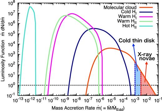
The distribution of the normalized mass accretion rate |$\dot{m}$|. Each curve shows the accretion distribution in each medium. The orange-red, dark-blue, magenta, light-green, and turquoise solid curves show the number distribution of isolated BHs in the molecular clouds, cold |$\mathrm{H}{\, }{\small {I}{\,}}$|, warm |$\mathrm{H}{\, }{\small {I}{\,}}$|, warm |$\mathrm{H}{\, }{\small {II}{\,}}$|, and hot |$\mathrm{H}{\, }{\small {II}{\,}}$|mediums, respectively. The red and blue dashed lines represent the critical accretion rates required to produce X-ray novae (equation (44), for m = 15) and to have a standard disc part (equation 29, for m = 15 and n = 102 cm− 3), respectively.
Let us discuss the shape of the distribution functions in Fig. 2. The peak value of the distribution in each ISM medium is roughly evaluated by Npeak ∼ Nξ0h. For the hot |$\mathrm{H}{\, }{\small {II}{\,}}$|medium, the distribution shows a peaky shape. This is because the hot |$\mathrm{H}{\, }{\small {II}{\,}}$|medium has a larger sound velocity cs than the typical BH velocity v ∼ σv, and the distribution reflects only the BH mass distribution. According to the Galactic potential (19), the BH scaleheight with the velocity v ∼ σv = 40 km s− 1 is estimated as H(vz) ≃ 0.3 kpc. On the other hand, the scaleheight of the hot |$\mathrm{H}{\, }{\small {II}{\,}}$|medium is larger than the BH scaleheight (see Table 1), and the correction factor reduces to unity h = 1. Then, the peak value of the distribution of the hot |$\mathrm{H}{\, }{\small {II}{\,}}$|medium is given as Npeak ∼ 4 × 10⁷ (N/108)(ξ0/0.4)(h/1).
For the warm |$\mathrm{H}{\, }{\small {I}{\,}}$|and |$\mathrm{H}{\, }{\small {II}{\,}}$|mediums, the mass accretion distributions have a broader shape than that of the hot |$\mathrm{H}{\, }{\small {II}{\,}}$|medium because the sound velocities of these mediums are as large as that of the BH velocity, cs ≲ v ∼ σv. Therefore, the broadness reflects the velocity distribution. These mediums also have larger scaleheights than the BH scaleheight, and have no correction (h ∼ 1). However, due to the large dispersion, the peak values of the distributions are a bit smaller than the values estimated by ∼Nξ0.
The accretion distributions of the molecular clouds and the cold |$\mathrm{H}{\, }{\small {I}{\,}}$|medium show tails extending to the large accretion rate (|$\dot{m}\gtrsim 10^{-5}$| and 10−3, for the cold |$\mathrm{H}{\, }{\small {I}{\,}}$|medium and the molecular clouds, respectively). These tails are attributed to the density distribution. To estimate the peak values of the distributions, we should take the correction factor h into account because the molecular clouds and the cold |$\mathrm{H}{\, }{\small {I}{\,}}$|medium have smaller scaleheights than that of BHs, Hd < H(vz), which requires corrections of h ∼ 0.1–0.3.
3 X-RAY NOVAE PRODUCED BY ISOLATED BHS
We discuss the possibility that isolated BHs produce X-ray transient events, such as X-ray novae. In Section 2, we consider that the accretion discs formed around isolated BHs are ADAFs. However, when the accretion rate is larger than a critical value, the radiative cooling overcomes the advective one and the ADAF becomes a standard disc (Abramowicz et al. 1995). Furthermore, if the standard disc has a low temperature region enough to allow hydrogen to recombine, the disc suffers from the hydrogen-ionization instability and produces an X-ray transient event.
Before discussing the accretion disc structure in detail, we check whether our idea passes the observational constraints. As shown in Fig. 2 and we discuss below, X-ray novae from isolated BHs occur only in molecular clouds because a large accretion rate is necessary. Then, if an X-ray nova is actually powered by an isolated BH, we should detect it in the same direction of a molecular cloud.2 We check an X-ray nova catalogue (Corral-Santana et al. 2016) and find 17 events in the Galactic plane (b ≲ 1.5°) among 59 X-ray novae ever detected. Comparing the CO emission map in the Galactic plane,3 we find CO emission signatures in the same directions of 16 X-ray novae. Furthermore, the 16 X-ray novae show large column densities of ∼ 1022 cm− 2 in the soft X-ray spectra, which also support that the 16 X-ray novae are actually accompanied with molecular clouds (see also Section 4). We list the 16 candidate X-ray novae in Table 2. The column density and direction are taken from the catalogue of Corral-Santana et al. (2016), and references therein. Therefore, we conclude 16/59 ∼ 0.27 of the observed X-ray novae are potentially produced by isolated BHs in molecular clouds.
Candidates X-ray novae powered by isolated BHs in molecular clouds. ID number corresponds to that used in Corral-Santana et al. (2016). The column density and direction are taken from Corral-Santana et al. (2016), and references therein. The column density is evaluated by the absorption signature in the soft X-ray spectra, except for ID47, 28, 22, 11, and, 2, for which the optical extinction formula NH = 5.8 × 10²¹E(B − V) cm− 2 is used (Draine 2011). In the same direction of each event, we find that there is a molecular cloud by checking the CO emission map. NIR counterparts are detected only for ID59, 35, and 34.
| ID | name | NH (cm− 2) | direction (l, b) | NIR source |
|---|---|---|---|---|
| 59 | IGR J17454−2919 | 1.0-1.2 × 10²³ | 359.6444, −00.1765 | |$\checkmark$| |
| 56 | SWIFT J1753.7−2544 | 5.8 × 10²² | 003.6476, +00.1036 | |
| 51 | MAXI J1543−564 | 1.4 × 10²² | 325.0855, −01.1214 | |
| 47 | XTE J1652−453 | 5.1 × 10²² | 340.5297, −00.7867 | |
| 44 | SWIFT J174540.2−290005 | 7.6 × 10²² | 359.9495, −00.0431 | |
| 43 | IGR J17497−2821 | 4.8 × 10²² | 000.9531, −00.4527 | |
| 35 | XTE J1908+094 | 2.3 × 10²² | 043.2615, +00.4377 | |$\checkmark$| |
| 34 | SAX J1711.6−3808 | 2.8 × 10²² | 348.4200, +00.7880 | |$\checkmark$| |
| 28 | XTE J1748−288 | 5.8 × 10²² | 000.6756, −00.2220 | |
| 25 | GRS 1737−31 | 6.0 × 10²² | 357.5880, −00.0990 | |
| 24 | GRS 1739−278 | 1.6 × 10²² | 000.6721, +01.1758 | |
| 23 | XTE J1856+053 | 4.5 × 10²² | 038.2690, +01.2720 | |
| 22 | GRS 1730−312 | 3.2 × 10²² | 356.6877, +01.0065 | |
| 11 | EXO 1846−031 | 3.7 × 10²² | 029.9585, −00.9177 | |
| 8 | H 1743−322 | 2.2 × 10²² | 357.2552, −01.8330 | |
| 2 | 4U 1630−472 | 2.4 × 10²² | 336.9112, +00.2503 |
If |$\dot{m}\gtrsim \dot{m}_{\rm {crit}}$|, the radiative cooling overcomes the advective cooling and no longer the ADAF part exists. Observations of BH X-ray binaries also suggest an outer standard accretion disc truncated in the inner part by radiatively inefficient accretion flow, which can explain some properties of BH X-ray binaries such as the spectral transition between the high-soft state and the low-hard state (Esin, McClintock & Narayan 1997; Lasota 2001; Done, Gierliński & Kubota 2007).
We conclude that isolated BHs with a mass accretion rate larger than the critical rates (29) and (44) suffer from the hydrogen-ionization instability and cause transient events such as X-ray novae. In Fig. 2, we show the population that causes transients with a red shaded region. We see that the number of the isolated BHs that can produce X-ray novae-like transients by the ionization instability is about NBH ∼ 20. BHs in a blue shaded region have mass accretion rates of |$\dot{m}_{\rm {disc}}<\dot{m}<\dot{m}_{\rm {crit}}^{-}(r=r_{\rm {tr}})$|. In this case, the whole region of the thin disc parts is always in the cold branch and stable (Menou, Narayan & Lasota et al. 1999).
The X-ray novae powered by isolated BHs show similar time-scale and luminosity to the observed ones. We briefly estimate the rise and decay time-scales and the luminosity of the X-ray novae. Before the detailed estimation, we remark that the accretion rate (|$\dot{m}\gtrsim 3\times 10^{-3}$|, see also Fig. 2) and the disc radius (Rd ∼ 1011 cm for V ∼ 10 km s− 1) of the isolated BHs are comparable to those of the X-ray binary system (van Paradijs 1996; Remillard & McClintock 2006; Coriat, Fender & Dubus 2012), which means that the accretion discs in both systems have common properties and show the common outburst signatures. The rise-time is evaluated by the time-scale for which a heating-front with velocity ∼αcs, disc propagates the disc radius (Lasota 2001), as trise ∼ Rd/αcs, disc ∼ 10 d (Rd/1011 cm)(α/0.1)− 1(cs, disc/10 km s− 1)− 1, where cs, disc is the sound velocity of the disc. The decay-time is estimated by the viscous time-scale as |$t_{\rm {decay}}\sim {t_{\rm {vis}}}\sim {R_{\rm {d}}^2}/3\nu _{\rm {vis}}$|, where νvis ≃ αcs, discHdisc is the kinetic viscosity, and Hdisc is the disc scaleheight at the disc radius (King & Ritter 1998). Then, the decay time-scale is given by tdecay ∼ 40 d (Rd/1011 cm)2(α/0.1)− 1(cs, disc/10 km s− 1)− 1(Hdisc/0.1Rd)− 1. Finally, since the outburst luminosity is evaluated by |$L_{\rm {burst}}\sim \eta \dot{M}_{\rm {burst}}c^2$|. The accretion rate is given by |$\dot{M}_{\rm {burst}}\sim {M_{\rm {d}}}/t_{\rm {vis}}$|, where |$M_{\rm {d}}\sim \pi {\Sigma }R_{\rm {d}}^2$| is the disc mass at the beginning of the outburst and Σ is the surface density at the cold branch of the S-curve. The surface density is obtained by solving the disc structure, but we evaluate it by using the fitting formula developed by Lasota, Dubus & Kruk (2008, ; their equation A.1) as Σ ∼ 6 × 10² g cm−2 (α/0.1)−0.83(Rd/1011 cm)1.18(MBH/10 M⊙)−0.40. Then, the accretion rate and the luminosity are estimated as |$\dot{M}_{\rm {burst}}\sim 6\times 10^{18}{\, }{\rm {g{\, }s^{-1}}}{\, }(\Sigma /6\times 10^2{{\, }\rm {g{\, }cm^{-2}}})(R_{\rm {d}}/10^{11}{\, }{\rm {cm}})^2(t_{\rm {vis}}/3\times 10^6{\, }\rm {s})^{-1}$| and |$L_{\rm {burst}}\sim 5\times 10^{38}{\, }{\rm {erg{\, }s^{-1}}}{\, }(\dot{M}_{\rm {burst}}/6\times 10^{18}{\, }{\rm {g{\, }s^{-1}}})\sim 0.4{\, }L_{\rm {Edd}}$| for MBH = 10 M⊙, where |$L_{\rm {Edd}}=\eta \dot{M}_{\rm {Edd}}c^2$| is the Eddington luminosity. The above estimated values of the rise and decay time-scales and luminosity agree with the observed values of trise ∼ 10 d, tdecay ∼ 30 d, and Lburst ∼ 0.1 LEdd (Chen, Shrader & Livio 1997; Yan & Yu 2015).
4 DISCUSSION
We discuss the observational strategy to confirm whether an X-ray nova is produced by an isolated BH or not. The simplest way is to exclude companion (or secondary) stars by follow-up observation. Typically, secondary stars of BH LMXBs are K- or M-type dwarves (Remillard & McClintock 2006). Their effective temperature and radius are about Teff ∼ 4000 K and R* ∼ 0.5 R⊙ (Torres, Andersen & Giménez 2010).
Then, we estimate the apparent magnitudes for optical V (λV = 0.545 μm) and near-infrared J (λJ = 1.215 μm), H (λH = 1.654 μm), and Ks bands (|$\lambda _{K_s}=2.157{\, }\rm {\mu {m}}$|) of the companion stars taking the extinction into account. We set the distance to an isolated BH as d ∼ 4 kpc, which is a typical distance to dynamically confirmed BHs (Corral-Santana et al. 2016). For this distance, the hydrogen column density contributed from the interstellar space amounts to NH ∼ 1.2 × 10²²(n/1 cm− 3)(d/4 kpc) cm− 2, where n denotes the number density of the interstellar space. On the other hand, the column density of the molecular clouds, where the BH resides, is NH ∼ 0.9 × 10²²(n/102 cm− 3)(l/30 pc) cm− 2, where we use a typical molecular cloud size of l ∼ 30 pc (Miville-Deschênes, Murray & Lee 2017). We see that these contributions are comparable, and we set the total column density as NH = 2 × 1022 cm− 2 to estimate the extinction. For the column density, the extinction of each band results in AV ≃ 12, AJ ≃ 3.2, AH ≃ 2.0, and |$A_{K_s}\simeq 1.4{\, }\rm {mag}$|, where we use Aλ/NH ≃ 6.0, 1.6, 1.0, and 0.7 × 10− 22 cm2 mag for V, J, H, and Ks bands, respectively (Draine 2003). Then, the apparent magnitudes in these bands become V ≃ 33.6, J ≃ 23.4, H ≃ 22.3, and Ks ≃ 21.9 mag. We find that optical follow-up observations are extremely difficult to detect secondary stars.
We discuss an observational strategy to confirm the absence of companions in near-infrared bands. When an X-ray nova is produced by a binary system, we can find the secondary star by deep near-infrared follow-ups. In the actual observations, we can use rough estimations of the column density by using the absorption signature of the soft X-ray spectrum (Liu, van Paradijs & van den Heuvel 2007; Corral-Santana et al. 2016, and references therein), in order to evaluate the necessary depths for follow-ups. In Fig. 3, we show the required depth to detect companion stars if they exists. Some observed X-ray novae whose column densities are evaluated by fitting of the absorbed soft X-ray spectrum (Corral-Santana et al. 2016, and references therein) are also shown. The selected X-ray novae are located at the low Galactic latitude position b ≲ 1.5° because their host molecular clouds have small scaleheights (see Table 1). Horizontal dotted lines represent the column density of each transient. Red, green, blue, and magenta curves show the estimated apparent AB magnitude, when the companions are located at 4 kpc from Sun, including extinction in V, J, H, and Ks bands, respectively. For example, MAXI J1543-564 has a column density of ≃ 1.4 × 1022 cm− 2. With this density, we should conduct follow-up observations as deep as ∼22.5, 21.6, and 21.4 mag in J, H, Ks bands. If we cannot detect any sources, the transient could be launched by an isolated BH.
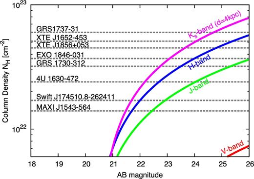
The required depth to detect the companion stars of the observed X-ray novae with the measured column densities. Red, green, blue, and magenta curves show the apparent magnitude of the companion stars, when the companions whose temperature and photospheric radius of Teff ∼ 4000 K and R* ∼ 0.5 R⊙, are located at 4 kpc from Sun. The horizontal dotted lines represent the measured column densities for X-ray novae that are not confirmed to have companions.
It should be also noted that a detection of near-infrared sources does not necessarily mean the existence of the companion. We also detect the disc as a near-infrared source. In this case, we should conduct spectroscopic observations. When the near-infrared source is not the companion but the disc emission of an isolated BH, we do not detect any periodic variation of emission or absorption lines (e.g. HI and HeII emission lines, or neutral metals and molecular absorption lines, as actually observed in BH binary systems, see e.g. Khargharia, Froning & Robinson 2010). In a catalogue of BH X-ray novae (Corral-Santana et al. 2016), such near-infrared candidate sources without periodic variabilities have been already reported, e.g. IGR J17454−2919, XTE J1908−094, and SAX J1711.6−3808. Among these X-ray novae, IGR J17454-2919 (Paizis et al. 2015) and SAX J1711.6−3808 (Wang & Wang 2014) are located at the same positions where the near-infrared sources have already been detected in the past survey observations, although the positions are crowded with stars and the chance of coincidence is high. Further follow-up observations are not conducted. For the other X-ray nova, XTE J1908−094 (Chaty, Mignani & Israel 2006), only photometric observations were conducted, and any detections of periodic variabilities were not reported. We should conduct deeper and more careful photometric and spectroscopic observations for these objects.
Radio follow-up observations are also important to study whether the transients are accompanied by molecular clouds or not. For example, the X-ray source 1E 1740.7−2942 in the Galactic centre was first proposed to be in a giant molecular cloud by radio observations (Bally & Leventhal 1991; Mirabel et al. 1991), but later shown to be located behind the cloud by detailed X-ray spectroscopic observations (Churazov, Gilfanov & Sunyaev 1996).
We also discuss the feedback effect of isolated BHs on the event rate. Theoretical studies suggest that ADAF solutions allow outflows from the disc systems (Blandford & Begelman 1999, 2004; Yuan et al. 2015). Even if a small fraction of accretion mass is blown away, the outflow affects the medium around the Bondi radius (Ioka et al. 2017). When the feedback works, the accretion rate is decreased, which also makes the outflows weak. Ioka et al. (2017) estimated the duty cycle of the self-regulation is about ∼1/10. In this case, the event rate of X-ray novae produced by isolates BHs will be decreased by ∼1/10.
When an X-ray flux from the inner disc part is large, it may affect the disc structure (van Paradijs 1996). The X-rays ionize hydrogen and the Saha equation (30) does not give a correct degree of ionization. Dubus et al. (1999) studied the effect of the X-ray irradiation and concluded that the disc structure or the S-curve does not change so much in the quiescent state. However, if the accretion disc is warped or there is a X-ray irradiation source above the disc plane, the X-ray ionization may affect the hot branch in the S-curve. This is an interesting future work.
Finally, we remark the difference between our work and Agol & Kamionkowski (2002), who also discussed a probability that isolated BHs launches X-ray novae. They calculated the event rate of X-ray novae produced by isolated BHs by using the mass accretion distribution. Their calculation predicted much more event rate than the observed one, and they concluded that X-ray novae caused by isolated BHs are unlikely. However, they did not consider the disc structure and the instability condition, and extremely underestimate the minimum accretion rate needed to produce X-ray novae. This is why, Agol & Kamionkowski (2002) overestimated the event rate of X-ray novae powered by isolated BHs.
ACKNOWLEDGEMENTS
We are thankful to Aya Bamba and Shota Kisaka for fruitful discussions and comments. We would like to thank Hitoshi Negoro for carefully reading the manuscript and giving us useful comments. We also thank Kengo Tachihara, Rei Enokiya, Shu Masuda, and Shogo Kobayashi for kindly helping us to check the CO observation map. TM is especially thankful to Takashi Hosokawa for helpful discussions and daily encouragements. This work is supported by Grant-in-Aid for JSPS Research Fellow 17J09895 (TM), KAKENHI 24000004, 24103006, 26247042, 26287051, 17H01126, 17H06131, 17H06357, and 17H06362 (KI).
Footnotes
Some literatures define the Eddington accretion rate without the radiative efficiency η. It should also be noted that the name ‘radiative efficiency’ does not mean the true efficiency.
Since it is difficult to measure the distance to an X-ray nova only by X-ray observations, we cannot study whether the X-ray nova actually reside in a molecular cloud. Therefore, we only discuss the coincidence of the directions of X-ray novae and molecular clouds.
At the outer part of the ADAF (r ≳ 100), the Coulomb collision works well and makes the electron temperature equal to the ion temperature.
In the hydrogen-ionization instability, the viscous parameter α is assumed to change between the hot and cold branches of the S-curve, in order to explain the outburst amplitude (Mineshige & Osaki 1983; Meyer & Meyer-Hofmeister 1984; Smak 1984). The change of the viscosity parameter is also supported by the detailed analysis of the dwarf-nova observations (Kotko & Lasota 2012), and magnetohydrodynamic simulations of accretion discs (Coleman et al. 2016). In our estimate, we use the viscous parameter α = 0.1 in the hot branch.
When hydrogen recombines and makes the opacity large, convection develops in accretion discs, which decreases the vertical temperature gradient (Meyer & Meyer-Hofmeister 1982; Cannizzo & Wheeler 1984). Therefore, if the convective motion reaches the midplane of the disc, the standard disc formula (32) overestimates the disc temperature. However, Cannizzo & Wheeler (1984) shows that the convection does not reach the midplane at the maximum accretion rate of the S-curve middle branch.
It should be noted that Lasota, Dubus & Kruk (2008) mainly studies the stability of helium accretion discs. However, in the Appendix of their paper, they show the fitting formulae for the solar abundance disc, which we use in this work.
REFERENCES
