


ABSTRACT
We present the latest results of a semi-analytic galaxy formation model, ‘New Numerical Galaxy Catalogue’, which utilizes large cosmological N-body simulations. This model can reproduce many statistical properties of galaxies at z ≲ 6. We focus on the properties of active galactic nuclei (AGNs) and supermassive black holes, especially on the accretion time-scale on to black holes (BHs). We find that the number density of AGNs at z < 1.5 and at hard X-ray luminosity <1044 erg s−1 is underestimated compared with recent observational estimates when we assume the exponentially decreasing accretion rate and the accretion time-scale which is proportional to the dynamical time of the host halo or the bulge, as is often assumed in semi-analytic models. We show that to solve this discrepancy, the accretion time-scale of such less luminous AGNs should be a function of the BH mass and the accreted gas mass. This time-scale can be obtained from a phenomenological modelling of the gas angular momentum loss in the circumnuclear torus and/or the accretion disc. Such models predict a longer accretion time-scale for less luminous AGNs at z < 1.0 than luminous QSOs whose accretion time-scale would be 107–8 yr. With this newly introduced accretion time-scale, our model can explain the observed luminosity functions of AGNs at z < 6.0.
1 INTRODUCTION
Galaxies are one of the main components of the Universe. Understanding galaxy formation and evolution is thus one of the main goals of astrophysics. Almost all galaxies have a supermassive black hole (SMBH) at their centre and the mass of SMBHs correlates with properties of their host galaxies, such as the mass and velocity dispersion of the bulges (e.g. Magorrian et al. 1998; Ferrarese & Merritt 2000; Häring & Rix 2004; McConnell & Ma 2013). SMBHs and their host galaxies would thus have co-evolved with each other. The gas can lose its momentum via the growing processes of the bulge and/or galactic bars, and a part of the gas would get accreted on to the SMBH (e.g. Mihos & Hernquist 1994; Wada & Habe 1995), which could be observed as active galactic nuclei (AGNs). After that, AGN radiation, jets, and outflow inject the energy and/or angular momentum to the surrounding gas, which would cause the increase/decrease of the star formation rate (SFR) of their host galaxies (e.g. Wagner et al. 2016, for a review). This ‘co-evolution’ is a standing question in astrophysics, and has been the subject of theoretical and observational studies over three decades. Such work has focused on the mechanism of black hole (BH) feeding and the energetic feedback related with BH growth in the context of galaxy formation (see, however, Jahnke & Macciò 2011).
Understanding the growth mechanisms and evolution of SMBHs is challenging because they cannot be directly observed. AGNs are the main sources to obtain information on SMBHs observationally, which emit light when material is accreted on to the SMBHs. To overcome the difficulty in investigating growth mechanisms and evolution of SMBHs, we need close comparisons between model predictions and observations of both galaxies and AGNs.
Semi-analytic models of galaxy formation (hereafter SA models) are powerful tools for making theoretical predictions that can be directly compared with observations. In SA models, merging histories of dark matter (DM) haloes are obtained from N-body simulations (e.g. Roukema et al. 1997; Okamoto & Nagashima 2003; Nagashima et al. 2005; De Lucia et al. 2010; Guo et al. 2016; Makiya et al. 2016) or analytic algorithms based on the extended Press–Schecter formalism (e.g. Press & Schechter 1974; Lacey & Cole 1993; Nagashima & Yoshii 2004; Menci et al. 2005; Valiante et al. 2011). The evolution of baryonic components such as gaseous haloes, galaxies, and SMBHs is followed by phenomenological modellings to diminish the computational cost and to enlarge the sample size. Therefore, SA models are an excellent approach for statistical studies of galaxies and SMBHs and particularly useful for theoretical studies of rare objects, such as AGNs.
There are a large number of previous studies using SA models aimed at revealing the evolution of SMBHs within their host galaxies. The evolution of the AGN luminosity function (LF), which has been well known to imply the ‘anti-hierarchical trend’ of SMBH growth, is regarded as one of the main observational constraints on the models. In the earlier studies, they tested the ‘merger-driven AGN scenario’ by comparing their QSO LFs with observational ones in optical bands (e.g. Kauffmann & Haehnelt 2000; Enoki, Nagashima & Gouda 2003). Other triggering mechanisms of AGN activities such as disc instabilities (e.g. Lagos, Cora & Padilla 2008; Fanidakis et al. 2011; Hirschmann et al. 2012), direct accretion from its hot gas halo (e.g. Fanidakis et al. 2012; Griffin et al. 2018), and galaxy–galaxy interactions (e.g. Menci et al. 2014) are also studied. Some authors investigated the SMBH and AGN growth over cosmic time (e.g. Fontanot et al. 2006; Monaco, Fontanot & Taffoni 2007; Marulli et al. 2008; Fanidakis et al. 2012; Enoki et al. 2014; Menci et al. 2014), the effect of BH spins (e.g. Lagos, Padilla & Cora 2009; Fanidakis et al. 2011; Griffin et al. 2018), the effect of the seed BH mass (e.g. Volonteri & Natarajan 2009; Shirakata et al. 2016), and AGN clustering (e.g. Fanidakis et al. 2013; Oogi et al. 2016, 2017).
There are, however, uncertainties related with phenomenological modellings of the SMBH evolution, e.g. the triggers and the duration of gas accretion, the relation between the accretion rate and the AGN luminosity, the dust attenuation, Compton absorption, BH seeding, and AGN feedback. Unfortunately, several physical processes degenerate. Different combinations of phenomenological modellings and free parameters in a model could equally well explain observational properties of AGNs. Therefore, it is important to understand the effect of each phenomenological modelling on properties of SMBHs and AGNs.
In this paper, we focus on the accretion time-scale on to SMBHs. Estimation of this time-scale is important as it reveals the co-evolution between SMBHs and their host galaxies. If all galaxies have undergone the AGN phase, the duration of this phase should be short to explain the observed AGN LFs. In contrast, AGNs should be long-lived if a small fraction of galaxies have experienced this phase (e.g. Soltan 1982).
There are some constraints on the accretion time-scales obtained from previous studies (see Martini 2004, for more details). Yu & Tremaine (2002) estimate the time-scale by comparing present-day mass density of BHs with the integrated accreted mass density in luminous AGN phases obtained from optical AGN LFs at various redshifts. They suggest that the average ‘AGN lifetime’ is 3–13 × 107 yr for |$10^{8-9} \, \mathrm{M}_\odot$| BHs if the radiation efficiency, ε, is 0.1–0.3. On the theoretical side, Kauffmann & Haehnelt (2000, hereafter KH00) estimate the AGN lifetime by using an SA model. They assume a constant radiation efficiency for AGNs, which are triggered only by major mergers of galaxies. They derive the average AGN lifetime to explain observed AGN LFs with MB ≲ −23 (where MB is the B-band absolute magnitude). They suggest that the lifetime is ∼3 × 10⁷ yr at z = 0 and that the time-scale would scale with the dynamical time of the halo; ∝ (1 + z)−1.5.
In these studies, the AGN lifetime is assumed to be the time-scale within which SMBHs are observed as optical AGNs. This time-scale is not necessarily equal to the accretion time-scale on to SMBHs. Hopkins et al. (2005) estimate not the AGN lifetime but the ‘total’ accretion time-scale considering the obscured accretion phases by using hydrodynamic simulations. They suggest that the accretion on to an SMBH is not visible at first because gas and dust components are surrounding the nuclear region. After blowing out these components by AGN winds, AGNs can be observed as optical sources. The AGN lifetime is then ∼20 Myr and the total accretion time-scale is ∼ 100 Myr for AGNs with MB < −22.
There are still two uncertainties about the accretion time-scale. One is the physical processes that govern the time-scale. Several authors have proposed different mechanisms that determine the accretion time-scale. KH00 suggest it is proportional to the dynamical time of the host halo. Norman & Scoville (1988) propose that the gas accretion continues during a starburst in its host galaxy, because they assume that the gas fuelling to an SMBH is promoted by the mass-loss from large star clusters. Granato et al. (2004) and Fontanot et al. (2006) assume the accretion rate to be determined by the viscosity of the accretion disc. The effect of these different assumptions on statistical properties of AGNs and SMBHs remains unclear.
It is also unclear whether the time-scale of less luminous AGNs is the same order as that of luminous ones. Previous work has focused on the time-scale of optical AGNs with MB < −22 (hard X-ray (2–10 keV) luminosity, LX, corresponds to ∼5 × 1043 erg s−1), whose SMBH mass is larger than |${\sim } 10^8 \, \mathrm{M}_\odot$|. Less luminous AGNs with LX ≲ 1044 erg s−1 would have wide range of SMBH masses. The accretion time-scale of such less luminous AGNs is not necessarily in the same order as luminous AGNs.
In this paper, we test a new phenomenological and physically motivated model of the accretion time-scale and investigate whether the effect of the accretion time-scale can explain the cosmic evolution of the AGN number density. We employ a revised version of an SA model, ‘New Numerical Galaxy Catalogue’ (hereafter ν2GC; Makiya et al. 2016, hereafter M16). The model more accurately explains statistical properties of galaxies and AGNs at various redshifts than the model of M16. We show the statistical properties of AGNs and SMBHs obtained by the model. This paper is organized as follows. In Section 2, we present the details of the modellings which is relevant to the growth of SMBHs and their host bulges. In Section 3, we present the statistical properties of model SMBHs and AGNs. We mainly focus on the effect of the accretion time-scale on AGN properties. Finally, in Section 4, we discuss and summarize the results.
2 MODEL DESCRIPTIONS
We create merging histories of DM haloes from large cosmological N-body simulations (Ishiyama et al. 2015),2 which have higher mass resolution and larger volume compared with previous simulations (e.g. four times better mass resolution compared with Millennium simulations, Springel et al. 2005). Table 1 summarizes basic properties of the simulations. The ν2GC-M, and -SS simulations have the same mass resolution with different box sizes (L = 560 and 70 h−1 Mpc, respectively). The ν2GC-H2 simulation is one of the high-resolution simulations for our SA model which has ∼64 times higher mass resolution than the ν2GC-SS simulation with the same box size. Throughout this paper, we assume a ΛCDM Universe with the following parameters: Ω0 = 0.31, λ0 = 0.69, Ωb = 0.048, σ8 = 0.83, ns = 0.96, and a Hubble constant of H0 = 100 h km s−1 Mpc−1, where h = 0.68 (Planck Collaboration I 2014; Planck Collaboration XIII 2016).
Properties of the ν2GC simulations we have employed in this paper. N is the number of simulated particles, L is the co-moving box size, m is the individual mass of a dark matter particle, Mmin is the mass of the smallest haloes (=40 × m) which corresponds to the mass resolution, and Mmax is the mass of the largest halo in each simulation.
| Name | N | L (h−1 Mpc) | |$m\,(h^{-1} \, \mathrm{M}_\odot )$| | |$M_\mathrm{min}\,(h^{-1} \, \mathrm{M}_\odot )$| | |$M_\mathrm{max}\,(h^{-1} \, \mathrm{M}_\odot )$| |
|---|---|---|---|---|---|
| ν2GC-M | 40963 | 560.0 | 2.20 × 10⁸ | 8.79 × 10⁹ | 2.67 × 10¹⁵ |
| ν2GC-SS | 5123 | 70.0 | 2.20 × 10⁸ | 8.79 × 10⁹ | 6.58 × 10¹⁴ |
| ν2GC-H2 | 20483 | 70.0 | 3.44 × 10⁶ | 1.37 × 10⁸ | 4.00 × 10¹⁴ |
The model used in this work is based upon the original ν2GC model of M16, although it has undergone numerous improvements. This model originates from Nagashima & Yoshii (2004) and Nagashima et al. (2005) (νGC model). Both νGC and ν2GC models have been used for a variety of astrophysical studies including gravitational waves, Lyα emitters, star formation, and AGN clustering (Enoki et al. 2003; Enoki & Nagashima 2007; Kobayashi, Totani & Nagashima 2007; Makiya et al. 2014; Oogi et al. 2016, 2017). The SMBH growth and AGN properties in M16 are based on Enoki et al. (2003, 2014), and Shirakata et al. (2015). In this section, we describe the processes which relate to the growth of SMBHs (and their host bulges). Other modellings are shown in Appendix A. Schematics of the model are shown in Fig. 1. In our model, the values of adjustive parameters are determined by a Markov Chain Monte Carlo (MCMC) method. The details of fitting procedures, its result, and the resulting statistical properties of galaxies with the fiducial model are shown in Appendix B.
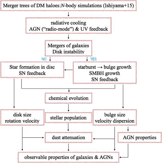
Schematics of the model showing the determination of observable properties of galaxies and AGNs.
2.1 Bulge growth by mergers and disc instability
We assume that the bulge (spheroid) component within a galaxy grows via starbursts and the migration of disc stars, both of which are triggered by mergers of galaxies and disc instabilities. Our model for these processes is based on Shirakata et al. (2016).
2.1.1 Mergers of galaxies
When DM haloes merge with each other, the newly formed halo should contain several galaxies which are classified as satellite galaxies and a single central galaxy. All members of this galaxy group would eventually merge under the gravitational attraction of the resultant halo. Mergers of galaxies occur via dynamical friction (central–satellite merger) and random collision (satellite–satellite merger). We estimate the time-scales of dynamical friction and random collision in the same manner as M16. For the dynamical friction, we set the merger time-scale, τmrg, as τmrg = fmrg τfric, where fmrg is an adjustable parameter (in this paper, fmrg = 0.81) and τfric is the time-scale of dynamical friction, for which we adopt the formula by Jiang et al. (2008) and Jiang, Jing & Lin (2010).3
These types of mergers induce bulge formation and growth within a galaxy. We introduce the model of the merger-driven bulge growth proposed by Hopkins et al. (2009a) based on hydrodynamic simulations. When galaxies merge, stars and gas lose their angular momentum through bar instabilities induced by the merger.
We define a primary galaxy as the galaxy with a larger baryon mass, M1 (cold gas + stars + a central BH), between the merging pair, and secondary galaxy as the one with smaller baryon mass, M2. We assume that the secondary is absorbed in the bulge of the primary. The bulge also obtains the cold gas and stars from the primary’s disc. The migrated stellar mass, ΔM1ds, is determined as MIN(f*M2, M1,ds), where f* = G(μ) = 2μ/(1 + μ) is the mass fraction of the disc that is destroyed as a function of μ = M2/M1 (Hopkins et al. 2009a). This results in the bulge of the primary gaining the stellar mass of M2 + ΔM1ds ≲ 2M2 per a merger.
As shown in equations (2) and (3), ΔM1dg is smaller than M1dg even when μ = 1 (i.e. an equal-mass merger). In this case, we cannot form pure bulge galaxies. We thus assume that the disc of the primary galaxy is completely destroyed when μ > fmajor, where fmajor is a free parameter (fmajor = 0.89). We then set ΔM1ds = M1ds and ΔM1dg = M1dg.
2.1.2 Disc instability
We also consider bulge growths via disc instabilities. When a galactic disc becomes gravitationally unstable, a small fraction, fbar, of the galactic disc is assumed to migrate to the bulge.
The critical value for disc stabilities, εDI,crit (equation 5), depends on the gas fraction and density profile of a galactic disc (e.g. Efstathiou et al. 1982; Christodoulou, Shlosman & Tohline 1995). If the velocity dispersion of galactic discs is neglected, the value of εDI,crit is ∼1.1 for the exponential stellar disc (Efstathiou et al. 1982) and ∼0.9 for the gaseous disc (Christodoulou et al. 1995). We, however, treat εDI,crit as an adjustable parameter, whose value should be ≤1.1 since the disc actually has the velocity dispersion and becomes more stable. We set εDI,crit = 0.75 to explain the observed cosmic SFR density. If we set εDI,crit = 1.1, the cosmic SFR density becomes constant at 4 < z < 6, which is inconsistent with the previous suggestions and such model cannot explain the observed stellar mass–SFR relation.
We note that some other SA models (e.g. Cole et al. 2000; Lacey et al. 2016) use the circular velocity and the half-mass radius of the disc instead of Vmax and rds. The circular velocity would change by the effect of the supernovae (SNe) explosions. We thus use Vmax following original prescription by Efstathiou et al. (1982). If we assume an exponential disc, the effective radius is only ∼1.67 times larger than the scale length.
The spheroids formed through this process might be so-called pseudo-bulges, although we do not differentiate between bulges formed by these instabilities and those formed by mergers. Starbursts triggered by these instabilities are also treated in the same way as those by mergers.
2.2 Growth of SMBHs and properties of AGNs
2.2.1 BH seeding
A seed BH is immediately placed within a newly formed galaxy. We use a mass of the seed BHs, |$M_\mathrm{BH,seed} = 10^{3} \, \mathrm{M}_\odot$|, for all galaxies independent from the redshift. The minimum mass of the halo in which the gas cools and possibly forms a galaxy depends on redshift and the mass resolution of N-body simulations (see fig. 2 in M16). A seed BH is therefore placed in a halo with different mass with different mass resolution and/or at different redshift. The seed BH mass, however, does not affect the main results of this paper, focusing mainly on AGNs at z ≲ 6, since the seed mass is negligible compared with the total amount of the accreted gas on to a BH (see Shirakata et al. 2016). Shirakata et al. (2016) suggest that the mass of the seed BHs should be dominated by |${\sim }\,10^3\, \mathrm{M}_\odot$| to reproduce the MBH−Mbulge relation at z ∼ 0, including galaxies with |$M_\mathrm{bulge}\,\lt \,10^{10} \, \mathrm{M}_\odot$|.
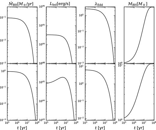
Examples of the growth history of model SMBHs with the initial SMBH mass of |$10^6 \, \mathrm{M}_\odot$|. We assume tacc = 107 yr and ΔMacc = 106 and |$10^7 \, \mathrm{M}_\odot$| in top and bottom panels, respectively. In this figure, we show the evolution of |$\skew4\dot{M}_\mathrm{BH}, L_\mathrm{bol}, \lambda _\mathrm{Edd},$| and MBH from left-hand to right-hand panels.
2.2.2 Mass accreted by SMBHs
We note that equations (12) and (13) are valid for SMBH growth via both galaxy mergers and disc instabilities. Practically, the value of fBH is not necessarily the same for both galaxy mergers and disc instabilities. There are, however, almost no suggestions about the difference of the fraction of the cold gas mass which gets accreted on to an SMBH with different triggering mechanisms. We, thus, employ the common fBH, for diminishing the degree of freedom.
SMBHs also increase their mass via SMBH–SMBH coalescence following mergers of galaxies. As in M16, we simply assume that SMBHs merge instantaneously after the merger of their host galaxies.
2.2.3 The accretion time-scale for SMBHs
In this paper, we test three types of the accretion time-scale summarized in Table 2. The KH00model, tacc = 3 × 10⁷ (1 + z)−1.5 yr, means that the accretion time-scale is proportional to the dynamical time of the host halo (originally introduced by KH00).
Summary of the accretion time-scale model (Section 2.2.3).
| Model name | tacc | Free parameters |
|---|---|---|
| KH00model | 3 × 10⁷(1 + z)−1.5 yr | None |
| Galmodel | αbulgetdyn,bulge | αbulge |
| GalADmodel | αbulgetdyn,bulge + tloss | αbulge, tloss,0, γBH, γgas |
| Model name | tacc | Free parameters |
|---|---|---|
| KH00model | 3 × 10⁷(1 + z)−1.5 yr | None |
| Galmodel | αbulgetdyn,bulge | αbulge |
| GalADmodel | αbulgetdyn,bulge + tloss | αbulge, tloss,0, γBH, γgas |
Some SA models (e.g. Fanidakis et al. 2012; Pezzulli et al. 2017) instead use the GalModel, tacc = αbulge tdyn,bulge by assuming the accretion continues until the gas supply from the host galaxy continues. The accretion time-scale is proportional to the dynamical time of the host bulge, tdyn,bulge = rb/Vb (where rb and Vb are the size and 3D velocity dispersion of the bulge, respectively), and the coefficient, αbulge, is a free parameter. We choose the value of αbulge so that the bright-end of the model AGN LFs are consistent with observed AGN LFs. In this paper, we set αbulge = 0.58.
When we use this model, we find that there are SMBHs whose accretion time-scale exceeds the age of the Universe. In this case, we set |$\skew4\dot{M}_\mathrm{BH} = 0$| implicitly assuming that accreted gas becomes gravitationally stable in a circumnuclear torus and/or a accretion disc, which cannot be accreted on to an SMBH. This treatment does not affect the shape of the AGN LFs since the accretion rates of such SMBHs are negligibly small.
There are some analytical estimates for the time-scale of the angular momentum loss in a circumnuclear torus (e.g. Kawakatu & Umemura 2002; Kawakatu & Wada 2008), which have been employed by some SA models (e.g. Antonini, Barausse & Silk 2015; Bromley, Somerville & Fabian 2004; Granato et al. 2004). We note that there are large uncertainties as to whether a circumnuclear torus with some common properties exists for all types of AGNs.
We do not consider an obscured phase (e.g. Hopkins et al. 2005), in which SMBHs do not appear as luminous AGNs at optical bands despite sufficiently large accretion rates on to SMBHs. To avoid this uncertainty, we compare the model results with observations by using AGN LFs in hard X-ray (2–10 keV) (see also Section 2.2.5).
2.2.4 AGN luminosity
2.2.5 ‘Observable fraction’ of AGNs
To compare the calculated AGN LFs with observed UV AGN LFs, we need to define ‘observable fraction’ in UV band, fobs,UV, because we can only obtain the intrinsic luminosity of AGNs from our model. Since AGN obscuration and absorption processes are very complicated, we derive an empirical formula by the following procedures. Recent work (e.g. Ueda et al. 2014; Aird et al. 2015) has estimated the hydrogen column density distribution around AGNs by a compilation of available samples obtained by Swift/BAT, MAXI, ASCA, XMM–Newton, Chandra, and ROSAT. Therefore, one can estimate the ‘intrinsic’ luminosity in hard X-ray of observed AGNs by utilizing the hydrogen column density distribution. We thus use the observed hard X-ray LFs (Aird et al. 2015, table 9) to obtain the ‘observable fraction’. The procedures are as follows.
Hopkins, Richards & Hernquist (2007) propose an alternative formula for the ‘observable fraction’. They employ an observed distribution of hydrogen column density and assume a dust attenuation curve, then they derive intrinsic AGN LFs in hard X-ray (2–10 keV), soft X-ray (0.5–2 keV), optical B, and mid-IR (15 |$\mu\mathrm{ m}$|). We show the difference between observable fractions obtained from Hopkins et al. (2007) and this paper in Appendix E.
Ricci et al. (2017) suggest that observed UV LFs of AGNs are well explained by their hard X-ray LFs, whose hydrogen column densities are less than 1021–22cm−2. Since the modelling of the distribution of gas around an SMBH is difficult for SA models, we estimate the observable fraction by an empirical formulation.
2.3 ‘Radio-mode’ AGN feedback
3 STATISTICAL PROPERTIES OF AGNS AND SMBHs
We present statistical properties of model AGNs and SMBHs, and show their dependence on the models of the accretion time-scale on to SMBHs. We first present the local SMBH MF in Fig. 3 and the MBH–Mbulge relation (including both AGNs and quiescent BHs) in Fig. 4. We show the results with the ν2GC-SS and ν2GC-H2 simulations in both figures for checking the effect of the mass resolution. The model SMBH MF at z ∼ 0 are shown as the grey dashed and black solid lines in Fig. 3. The SMBH MF is roughly consistent with the observational estimate (Shankar et al. 2004) (grey shaded region). The MBH–Mbulge relation at z ∼ 0 is consistent with observations at |$M_\mathrm{BH} \gt 10^{9.5} \, \mathrm{M}_\odot$| (Fig. 4) since we adjust the parameter, fBH, to reproduce this relation. We, however, find that the median value of the MBH–Mbulge relation obtained by the fiducial model deviates from the observational estimates for |$M_\mathrm{bulge} \lt 10^{9.5} \, \mathrm{M}_\odot$|. We do not use such low-mass galaxies for the model calibration since the observed sample is too small. Most observational data for less massive galaxies with |$M_\mathrm{bulge} \lt 10^{9.5} \, \mathrm{M}_\odot$| are AGN data. It is unclear whether the quiescent BHs with |$M_\mathrm{bulge} \lt 10^{9.5} \, \mathrm{M}_\odot$| have the same relation as the AGNs. In addition, the bulge mass of less massive galaxies is difficult to estimate by observations since the bulge is more rotational-support.
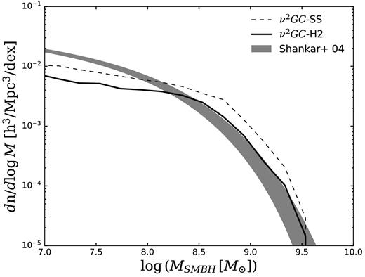
SMBH MF at z ∼ 0. The model result obtained with the ν2GC-SS and ν2GC-H2 simulations appear in grey dashed and black solid lines with analytical fit to the observational data obtained from Shankar et al. (2004) in grey shaded region.
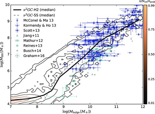
The relation between bulge mass and SMBH mass at z ∼ 0. The colour contour and black solid line show the distribution and the median value of mock galaxies obtained from the fiducial model with the ν2GC-H2 simulation, respectively. We overplot the result with the ν2GC-SS simulation, for checking the effect of the mass resolution. Blue filled triangles, circles, and squares are observational results for quiescent BH systems (Kormendy & Ho 2013; McConnell & Ma 2013; Scott, Graham & Schombert 2013, respectively). Cyan filled triangles, squares, diamonds, stars, and pluses are observational results for AGNs (Jiang, Greene & Ho 2011; Mathur et al. 2012; Reines, Greene & Geha 2013; Busch et al. 2014; Graham, Ciambur & Soria 2016, respectively).
3.1 The effect of the accretion time-scale on AGN LFs
We show the AGN properties obtained with ν2GC. We present the luminosity of AGNs in the hard X-ray (2–10 keV) band because the effect of obscuration and absorption is small. We show how AGN LFs change when we use three different models of the accretion time-scale in Fig. 5. Black lines show the model hard X-ray LFs with different accretion time-scales. We also show the fitting function of the LFs from Aird et al. (2015) with grey dotted lines and observed data from Aird et al. (2015), Ueda et al. (2014), and La Franca et al. (2005). We have confirmed that the results have no statistical differences when we employ the high-resolution N-body simulations.
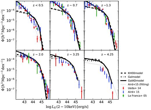
AGN LFs in hard X-ray (2–10 keV) at z < 0.5, z ∼ 0.7, z ∼ 1.3, z ∼ 2.0, z ∼ 3.25, and z ∼ 4.25. The model LFs are obtained with the ν2GC-M simulation. Black dashed, dot–dashed, and solid lines are the model LFs with different models of accretion time-scale; the KH00model, Galmodel, and GalADmodel, respectively. Observational results are obtained from red circles, blue triangles, and green squares are the data taken from Ueda et al. (2014), Aird et al. (2015), and La Franca et al. (2005), respectively. Grey dotted lines show the fitting LFs of observed data (Aird et al. 2015).
Black dashed lines show the hard X-ray (2–10 keV) AGN LFs with the KH00model, which is the time-scale proportional to the dynamical time of the host halo. The model is consistent with observational results at log (LX/erg s−1) > 43.5 within the dispersion of the observed data. We, however, find that the model underestimates the number density of AGNs at z < 1.0 with log (LX/erg s−1) < 43.5 (i.e. nuclei of Seyfert galaxies), whose UV (1450 Å) magnitude, MUV, corresponds to ∼−20.6. Such less luminous AGNs are not considered in the estimation of the AGN lifetimes in KH00 and their lifetimes could significantly differ for luminous AGNs.
Black dot–dashed lines show hard X-ray AGN LFs by the model in which the Galmodel. This modelling is similar to previous SA models (e.g. Fanidakis et al. 2012; Shirakata et al. 2016; Pezzulli et al. 2017). The accretion time-scale does not cause a big difference in the faint-end slope of AGN LFs compared with that with the KH00model, since the Galmodel has the accretion time-scale with the same order as the KH00model as shown later in Fig. 6.
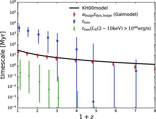
The redshift evolution of the accretion time-scale with KH00model, Galmodel, and tloss. The black solid line shows the KH00model, which corresponds to the dynamical time of haloes. The red circles and blue squares with error bars show the median value of tdyn,bulge and tloss of AGNs with log (LX/erg s−1) > 41.0 obtained by the GalADmodel. The errorbars are 25th and 75th percentiles. We also show the value of tloss of AGNs with log (LX/erg s−1) > 44.0 by green triangles.
Black solid lines show the hard X-ray AGN LFs with GalADmodel, implicitly considering the time-scale of angular momentum loss in the circumnuclear torus and the accretion disc. The model enables us to reproduce not only bright-ends of the LFs but also the faint-ends, especially at z < 1.5. When this model of the accretion time-scale is employed, a significant fraction of low-luminosity AGNs sustain their activity for a long time as we will show later. The model thus reproduces the both the bright- and faint-ends of AGN LFs much better than the other models.
Next, Fig. 6 shows the redshift evolution of the accretion time-scale of KH00model and Galmodel, and tloss. We select AGNs with log (LX/erg s−1) > 41.0. The red circles and blue squares with error bars show the median value of αbulgetdyn,bulge and tloss with 25th and 75th percentiles. The redshift evolution of the dynamical time of the bulge (red circles) and the halo (black solid line) are similar although the difference becomes larger at higher redshift. This explains why the AGN LFs with the KH00model and Galmodel are similar. While tloss distributes broadly, it is longer especially at lower redshift. This results in the increase of the number density of AGNs at log (LX/erg s−1) < 43.5 and z < 1.5. We also plot tloss only for luminous AGNs with log (LX/erg s−1) > 43.5 as green triangles. The time-scale is more than one order of magnitude shorter than that of AGNs with log (LX/erg s−1) > 41.0 at all redshifts.
The GalADmodel predicts the longer accretion time-scales for the less luminous AGNs due to the effect of tloss as shown in Fig. 7. This figure shows the relation between hard X-ray luminosity and time-scales (tloss and αbulgetdyn,bulge) at z ∼ 0, 2, and 4. We find that the time-scale is almost constant (∼2 × 10⁷ yr) for AGNs with log (LX/erg s−1) > 44.0 (corresponds to MUV < −22.3), which is consistent with the constraints obtained by previous studies (Yu & Tremaine 2002; Kauffmann & Haehnelt 2000; Hopkins et al. 2005). Less luminous AGNs, in contrast, have negative correlations between the time-scale and LX. We also find that the total accretion time-scale becomes longer at lower redshift for all AGNs.
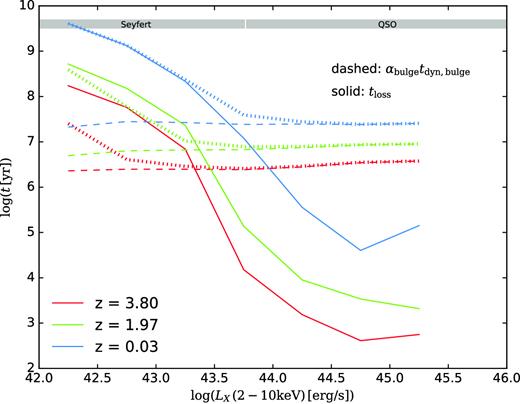
The relation between hard X-ray luminosity and two different time-scales at z ∼ 0, 2, and 4 (blue, green, and red lines, respectively) obtained with the GalADmodel. Solid and dashed lines describe tloss and αbulgetdyn,bulge, respectively.
The results obtained with the GalADmodel naturally explains the evolution of the AGN number density, which is sometimes called as ‘anti-hierarchical trend’ of SMBH growth. Fig. 8 shows the number density of AGNs obtained with the GalADmodel, and those obtained from observations (Ueda et al. 2014; Aird et al. 2015). The reason why the model result shows mild anti-hierarchical trends would be partially because we consider the obscured fraction in hard X-ray (2–10 keV) is 0 at all redshift. We will show a more detailed analysis in future.
![The redshift evolution of the AGN number density. Colour describes the luminosity bins (log (LX/ergs−1) = [42, 43], red; (log (LX/ergs−1) = [43, 44], yellow; (log (LX/ergs−1) = [44, 45], green; and (log (LX/ergs−1) = [45, 46], blue). The results obtained with GalADmodel are shown with lines. Filled squares with error bars and triangles are observational results (Ueda et al. 2014; Aird et al. 2015, respectively).](https://oup.silverchair-cdn.com/oup/backfile/Content_public/Journal/mnras/482/4/10.1093_mnras_sty2958/1/m_sty2958fig8.jpeg?Expires=1716540970&Signature=Oqh5hlVcDeGlRovvv80LNt000-6FCn5qrdkpuSrAtcQjGNdKofeXMGB5uCgdiHZWcWOtPrZwmwhx8wQ7OJxe0geICmG~TkKsd3c0yUF0JgmAr1onurG4cXbfhaPP67zomffRHcDgkOVlFJ~dkpiPDlYA7R17Rcr3PF4fFwSEhe1i6CE~IzTRfrXy8eBkB8TYp1xSsGWP7jCgWTSf5kRM1~rwVg5znobzKvwpfuBmhFS82xPQ82Ur-2i5hEBuCxqdTg9Q7STslxC4lv14OmSJQmNoArAZxQB4EikgkAvyX7qnJLCT7IM32gTKhwFA4-l2gaSduaFHrcQKbU6jm92j1w__&Key-Pair-Id=APKAIE5G5CRDK6RD3PGA)
The redshift evolution of the AGN number density. Colour describes the luminosity bins (log (LX/ergs−1) = [42, 43], red; (log (LX/ergs−1) = [43, 44], yellow; (log (LX/ergs−1) = [44, 45], green; and (log (LX/ergs−1) = [45, 46], blue). The results obtained with GalADmodel are shown with lines. Filled squares with error bars and triangles are observational results (Ueda et al. 2014; Aird et al. 2015, respectively).
3.2 The effect of the time-scale on other properties of AGNs
To see dependencies of the accretion time-scale on MBH and ΔMacc, we show the relation between AGN bolometric luminosity and BH mass, MBH (top panels), and accreted gas mass on to an SMBH, ΔMacc (bottom panels) at z ∼ 0, in Figs 9 and 10. In Fig. 9, x-axes are the AGN bolometric luminosity at t = tstart, Lbol(tstart), while these are AGN bolometric luminosity at the output time, Lbol(tout), in Fig. 10. The left-hand panels show the result with the Galmodel and the right-hand panels show that obtained by the GalADmodel. We note that the model AGNs have a weak correlation between MBH and ΔMacc, of the form |$M_\mathrm{BH} \propto \Delta M_\mathrm{acc}^{1.1}$|, with a large dispersion. This positive correlation comes from the fact that the host galaxy of the heavier SMBH is more massive and has large amount of the cold gas.
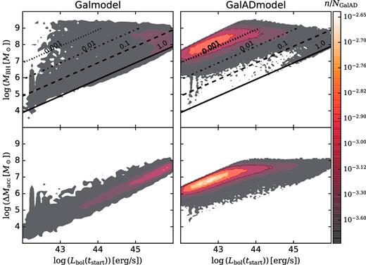
The relation between the AGN bolometric luminosity at t = tstart, Lbol(tstart), and BH mass, MBH (top) and accreted gas mass on to an SMBH, ΔMacc (bottom) at z ∼ 0. The distributions are described as density contours, whose value is normalized by the number of total AGNs with GalADmodel. Left-hand and right-hand panels show the results obtained with the Galmodel and GalADmodel, respectively. Black solid, dashed, dot–dashed, and dashed lines show λEdd = 1, 0.1, 0.01, and 0.001, respectively.
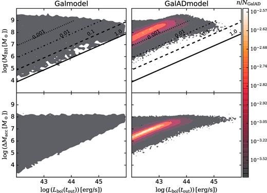
The same figure as 9 although the x-axis shows the AGN bolometric luminosity at output time, Lbol instead of Lbol,peak.
Fig. 9 shows the clear correlation between Lbol(tstart) and ΔMacc with the Galmodel (bottom left panel). Since tdyn,bulge is similar for galaxies at the same redshift (see Fig. 6), the peak accretion rate, |$\skew4\dot{M}_\mathrm{peak} \equiv \Delta M_\mathrm{acc} / t_\mathrm{acc}$|, is mainly determined by ΔMacc. The higher peak bolometric luminosity therefore implies a larger amount of the accreted gas. The relation between Lbol(tstart) and MBH with the same model (top left panel) comes from the correlation, |$M_\mathrm{BH} \propto \Delta M_\mathrm{acc}^{1.1}$|.
The correlations obtained by the GalADmodel (right-hand panels) show bimodal distributions, which are quite different from the model with the Galmodel. The peak accretion rate is proportional to |$M_\mathrm{BH}^{-\gamma _\mathrm{BH}} \Delta M_\mathrm{acc}^{1 - \gamma _\mathrm{gas}}$| if αbulgetdyn,bulge is smaller than tloss. Since γBH = 3.5 and γgas = −4.0, |$\skew4\dot{M}_\mathrm{peak} \propto M_\mathrm{BH}^{-3.5} \Delta M_\mathrm{acc}^{5.0}$|. The peak accretion rate, thus, can be written as |$\skew4\dot{M}_\mathrm{peak} \propto \Delta M_\mathrm{acc}^{1.15}$| (or |$\propto M_\mathrm{BH}^{1.05}$|). These positive correlations appear as contour peaks at log (Lbol(tstart)/erg s−1) < 44.0.
Fig 10 shows the same relations as shown in Fig. 9, but instead plotting bolometric luminosity estimated at an output time. Since Lbol(tstart) has positive correlations with MBH and ΔMacc when the Galmodel is employed, the dispersions of the correlation between Lbol and MBH and ΔMacc (left-hand panels) reflect the elapsed time from their AGN activity.
The relation between AGN luminosity and SMBH mass allows us to compare theoretical models with observations and to potentially place a stronger constraint on the accretion time-scale. There are numerous previous studies which present the relation between AGN luminosities and the SMBH mass at various redshifts (e.g. Schulze & Wisotzki 2010; Nobuta et al. 2012; Ikeda et al. 2017). Schulze & Wisotzki (2010) and Steinhardt & Elvis (2010) show the relation between the bolometric luminosity and the SMBH mass for broad line AGNs at z < 0.3 and 0.2 < z < 2.0, respectively. Since their sample are limited at λEdd > 0.01, we cannot distinguish the two models of the accretion time-scale. If complete AGN sample with λEdd > 0.001 are obtained, we could put a stronger constraint on the accretion time-scale.
In Fig. 11, we present AGN LFs in UV band (1450 Å) from z ∼ 6.0 to 0.0 obtained by the GalADmodel. The observable fraction is defined by equation (21). The results are roughly consistent with observed UV AGN LFs (Croom et al. 2001, 2009; Fan et al. 2001; Richards et al. 2005, 2006; Fontanot et al. 2007; Siana et al. 2008; Glikman et al. 2011; Fiore et al. 2012; Ikeda et al. 2012; Palanque-Delabrouille et al. 2013; Ricci et al. 2017; Akiyama et al. 2018), especially at z > 1.5. We, however, overproduce UV LFs at lower redshift. In such redshift range, we also overproduce hard X-ray LFs (see Fig. 5) compared with the fitting LFs of Aird et al. (2015) although the model LFs are consistent with observed data points within the range of a dispersion. We need to take the dispersion of observed hard X-ray LFs into account for estimating the observable fraction although we leave it for future studies. The UV LFs do not place a strong constraint on the accretion time-scale since the observed UV LFs are well determined only at MUV < −20.8 [corresponds to log (LX/erg s−1) > 44.6] because of the contamination of galaxies’ emission (Parsa et al. 2016). The hard X-ray LFs obtained from models with the different assumption of the accretion time-scale show little difference at log (LX/erg s−1) > 44.6.
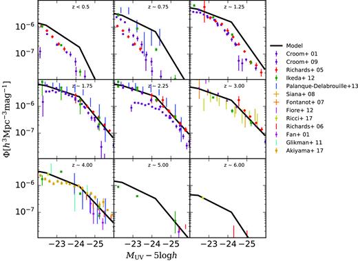
AGN LFs in UV band (1450 Å) at z < 0.5, z ∼ 0.75, z ∼ 1.25, z ∼ 1.75, z ∼ 2.25, z ∼ 3.00, z ∼ 4.00, z ∼ 5.00, and z ∼ 6.00. The model LFs (volume-weighted) obtained with the ν2GC-M simulation appear in black solid lines. Observational results are obtained from Croom et al. (2001, 2009), Fan et al. (2001), Richards et al. (2005, 2006), Fontanot et al. (2007), Siana et al. (2008), Glikman et al. (2011), Fiore et al. (2012), Ikeda et al. (2012), Palanque-Delabrouille et al. (2013), Ricci et al. (2017), and Akiyama et al. (2018).
We show Fig. 12 to show the effect of the time-scale on the Eddington ratio distribution function. The black solid and dashed lines are results obtained with GalADmodel and Galmodel, respectively. We select all AGNs with |$M_\mathrm{BH} \gt 10^6 \, \mathrm{M}_\odot$| and Lbol > 1043.5 erg s−1 at z ∼ 0. The results at log (λEdd) > −1.5 are roughly consistent with that obtained by the observation (Schulze & Wisotzki 2010) at z ∼ 0.3. We, however, note that it is difficult to compare model Eddington ratio distribution functions with observations since (1) optical observational sample is limited in type-1 AGNs with well-estimated SMBH mass, (2) SMBH masses of X-ray AGNs are simply estimated from e.g. the BH mass–stellar mass relation, (3) observational sample seems to be incomplete for less massive SMBHs, and (4) the obscured fraction of AGNs would depend on both their luminosity and Eddington ratio (e.g. Oh et al. 2015; Khim & Yi 2017). Also, if there is an obscured growing phase before visible AGN phase suggested by, e.g. Hopkins et al. (2005), then the super-Eddington accreting phase should be preferentially missed.
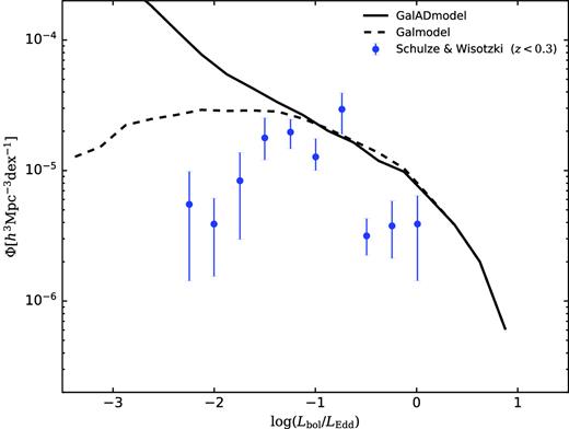
The Eddington ratio distribution functions at z ∼ 0 obtained with GalADmodel and Galmodel (black solid and dashed lines, respectively). In both models, AGNs with |$M_\mathrm{BH} \gt 10^6 \, \mathrm{M}_\odot$| and LX > 1043 erg s−1 are selected. Also, we compare the results with that obtained by Schulze & Wisotzki (2010) at z ∼ 0.3 (blue filled circles with error bars).
Fig. 12 clearly shows the difference caused by the implementation of the accretion time-scale. The GalADmodel increases the number of AGNs with log (λEdd) < −1.5 and the difference between the two models becomes larger at smaller Eddington ratio. We find that the GalADmodel and Galmodel have no difference for active BHMF with AGNs |$M_\mathrm{BH} \gt 10^6 \, \mathrm{M}_\odot$|, Lbol > 1043.5 erg s−1, and λEdd > 0.03 (roughly similar selection as that of Schulze & Wisotzki 2010). As we can expected from AGN LFs (Fig. 5), the Eddington ratio distribution functions at z > 1.0 also have little difference between the GalADmodel and Galmodel. The evolution of the Eddington ratio will appear in a future paper.
3.3 Triggers of the gas supply from host galaxies
Fig. 13 shows the fraction of AGN host galaxies at 0.0 < z < 7.0 in each luminosity bin, divided by triggering situations. We classify the galaxies by the mass ratio of the merging galaxies; major (mass ratio >0.7 = fmajor; blue dash dotted line), intermediate (0.4–0.7; green dotted line), and minor (<0.4; red solid line). The grey dashed line shows the fraction of AGNs triggered only by a disc instability. For merger-driven AGN activities, the typical merging mass ratio becomes larger for more luminous AGNs. Interestingly, we find that the primary trigger of AGNs at z < 4.0 is mergers of galaxies, although, at higher redshift, disc instabilities become essential for less luminous AGNs. This result is inconsistent with Fanidakis et al. (2012) and Griffin et al. (2018), who suggest that disc instabilities and ‘hot halo mode accretion’ are dominant triggering mechanisms of AGNs even at z < 4.0. As we described in Section 2.1, we employ the smaller εDI,crit for reproducing the properties of star formation galaxies at z > 4. Also, we consider the effect of the bulge potential on the stability of galactic discs. With this effect, the number of disc-unstable galaxies becomes 60 per cent smaller at z ∼ 1 with εDI,crit = 0.75. These are why our model suggests such low efficiency of disc instabilities as a triggering mechanism. The critical point is that the observed number density of AGNs can be sufficiently reproduced at z < 4 only by mergers of galaxies, and the importance of disc instabilities and other processes should be investigated in more detail. Our model predicts disc instabilities drive only less than 20 per cent of AGNs at z ∼ 0. We will come back this topic in Section 4.
![Fraction of the AGN host galaxies whose AGN activity is triggered by mergers of galaxies or disc instabilities. We pick out AGNs (in ν2GC-M box) with log (LX/ergs−1) = [41.5, 42.5], [42.5, 43.5], [43.5, 44.5], and >44.5. Mergers are classified according to the mass ratio of merging galaxies: >0.70 (major, blue dash–dotted), between 0.4 and 0.7 (middle, green dotted), and <0.4 (minor, red solid). We also show the fraction of AGNs triggered only by the disc instability (grey dashed).](https://oup.silverchair-cdn.com/oup/backfile/Content_public/Journal/mnras/482/4/10.1093_mnras_sty2958/1/m_sty2958fig13.jpeg?Expires=1716540970&Signature=VGfRr~lhLDXVzCuqaSjr7GEvmMmnr48ByP1y8OahRfQZK16xbFwbB9AuDPhnbrgbvXmW5KYMRqVofd15s5mplkoJtJvSv37s388k9Mi9MPxj50Rtet-LBc2k0z9cBhnki5BI6PhkFvl34eu0MEy3Da8AL4WStI7tY52C6LqEuwNoHI-GiWnuKu726Z389l4aSmH~lwslZGw~BY827yWDz6ohUIBr2Y988jTj9rrIaCniVVU6BErkWr8sqzngCkJiLYV0tqXKsWVhM~EfS4Wfr593mzNxHFHnNuAxWmDXrssOxDtcPXRUzqeOCxfoTuQb0CZ1Co6-Xz~0U1hNx7McPQ__&Key-Pair-Id=APKAIE5G5CRDK6RD3PGA)
Fraction of the AGN host galaxies whose AGN activity is triggered by mergers of galaxies or disc instabilities. We pick out AGNs (in ν2GC-M box) with log (LX/ergs−1) = [41.5, 42.5], [42.5, 43.5], [43.5, 44.5], and >44.5. Mergers are classified according to the mass ratio of merging galaxies: >0.70 (major, blue dash–dotted), between 0.4 and 0.7 (middle, green dotted), and <0.4 (minor, red solid). We also show the fraction of AGNs triggered only by the disc instability (grey dashed).
4 DISCUSSION AND CONCLUSIONS
We have presented the latest results of an updated version of an SA model, ν2GC. The most important changes are related to the bulge and SMBH growth model. We assume that the gas accretion on to the SMBH and the bulge growth are triggered by mergers of galaxies and disc instabilities. For bulge and SMBH growths by mergers of galaxies, we employ a phenomenological model proposed by Hopkins et al. (2009a), whose model is based on results of hydrodynamic simulations. Along with this revision, we have also updated the way of calculating the velocity dispersion and size of bulges when bulges grow via minor mergers. For bulge and SMBH growths by disc instabilities, we employ a classical model originally proposed by Efstathiou et al. (1982). We consider the effect of the bulge potential on the gravitational stability of the disc.
We have investigated the effect of the accretion time-scale on statistical properties of AGNs, such as their LFs. We stress that the impact of the accretion time-scale especially for low-luminosity (LX < 1044 erg s−1) AGNs has been almost neglected in previous SA models. When we assume that the accretion time-scale is proportional to the dynamical time of the host halo or the host bulge, as in the previous SA models, the number density of the low-luminosity AGNs is one order of magnitude smaller than observational estimates. We have found that the number density of such less luminous AGNs becomes consistent with the observational data when we take a phenomenological and physically motivated model for the time-scale of the angular momentum loss in the circumnuclear torus and/or the accretion disc into account. The GalADmodel predicts that low-luminosity AGNs at z < 1.0, such as local Seyfert-like AGNs, are mainly triggered by minor mergers. The contribution of disc instabilities is only less than 20 per cent.
Previous studies with SA models solve the inconsistent number density of less luminous AGNs by considering other AGN triggering mechanisms such as ‘efficient’ disc instabilities (e.g. Hirschmann et al. 2012), fly-by interactions of galaxies (e.g. Menci et al. 2014), and the direct gas accretion from the hot halo (e.g. Fanidakis et al. 2012, ‘hot halo mode’). Hirschmann et al. (2012) suggest the importance of disc instabilities as a triggering mechanism of less luminous AGNs. We, however, have to note that the phenomenological modelling of disc instabilities in SA models would be too simple and is not supported by numerical simulations (see Athanassoula 2008). We have tried to make more physically reasonable modelling of disc instabilities in this paper. For the first step, we include the stabilizing effect by the bulge component and take smaller εDI (Section 2.1.2). We then find that disc instabilities are not the main contributor to AGN triggering mechanisms. As another point, some SA models (e.g. Fanidakis et al. 2012; Griffin et al. 2018) assume that a disc instability destroys a galactic disc entirely and all the gas is exhausted by a starburst forming a spheroidal galaxy just as major mergers. By these two effects (ignoring bulge potential and the complete destruction of a disc), some SA models are likely to overproduce the number density of AGNs induced by disc instabilities. Further updates are necessary, and we leave it for future studies. Menci et al. (2014) suggest that fly-by interactions are important instead of disc instabilities. Although we do not introduce fly-by interactions, the random collision of galaxies may have similar effects. The ‘hot halo mode’ (Fanidakis et al. 2012; Griffin et al. 2018) is the same as our ‘radio-mode’ AGN feedback model, both of which are based on Bower et al. (2006). In our fiducial models, we do not calculate the AGN luminosity with this mode because the bolometric correction and the radiative efficiency are unclear. When we assume the same bolometric correction as that of QSOs, and the radiative efficiency is 0.1, the contribution of the radio-mode AGN to the AGN LFs becomes the same order as that of AGNs induced by mergers of galaxies and disc instabilities at LX ∼ 1041 erg s−1 at z ∼ 0. The contribution becomes smaller at more luminous regime and at higher redshift. Our results based on the time-scales show that observed AGN LFs can be reproduced without ‘radio-mode’ or ‘hot halo mode’ accretions. Even without the ‘radio-mode’ AGN feedback, GalADmodel produces a large number of AGNs with low Eddington ratios, which would be AGN jet and outflow sources. Considering the injected energy and momentum from the low Eddington ratio AGNs, they may have non-negligible impact on the star formation quenching of massive galaxies. We will examine which explanation is more plausible in a future study.
Marulli et al. (2008) suggest the importance of AGN light curve for determining the shape of AGN LFs. They assume three types of the Eddington ratio evolution models based on observations and hydrodynamical simulations. The faint end slope of AGN LFs at z < 1.0 are well fitted when they assume the constant Eddington ratio, namely, =0.3[(1 + z)/4]1.4 at z < 3, and =1 at z > 3. By using this Eddington ratio, the accretion time-scale should be ∼0.17 Gyr at z ∼ 0, which is larger than the dynamical time of bulges (Fig. 6) and is qualitatively consistent with our suggestion. However, the model with this assumption of the constant Eddington ratio underestimates the number density of luminous AGNs at z > 1. They also introduce AGN light curve with two stages; rapid, Eddington-limited growth phase, and longer quiescent phase with lower Eddington ratios. By using this light curve, the accretion time-scale should be longer when the SMBH mass is smaller or the accreted gas mass is larger, which is the opposite to that suggested in the GalADmodel. The resulting faint end slope of AGN LFs at z < 1 is shallower than observations. They cannot explain the shape of the AGN LFs by changing just the Eddington ratio distribution. Finally, they introduce SMBH mass dependence to the fBH and successfully reproduce AGN LFs at z < 5.
Hydrodynamic simulations (e.g. Hirschmann et al. 2014; Khandai et al. 2015; Sijacki et al. 2015) do explain AGN LFs well, assuming Bondi–Hoyle–Littleton (BHL) accretion for all SMBH growths. Generally, hydrodynamic simulations assume that the ‘effective’ accretion rate on to SMBHs is roughly 200 times larger than the BHL accretion rate, which is too small compared to that of observed AGNs (e.g. Ho 2009). The assumption of the accretion rate with ∼200 times larger than the BHL accretion, independent of any properties of galaxies and SMBHs, might be a too simplified assumption. Besides, we must care about another uncertainty; different AGN feedback models are employed in different cosmological simulations, which reproduce AGN LFs at the same extent.
As we have shown, there are several prescriptions to explain the faint end slopes of AGN LFs at z < 1. For discriminating the models, comparisons of model results with observed properties of AGNs and their host galaxies are necessary. We have shown the relation between MBH and LX (Figs 9 and 10), the Eddington ratio distribution function at z ∼ 0.3 (Fig. 12), and the fraction of AGNs with different triggering mechanisms (Fig. 13). Since the difference between the Galmodel and GalADmodel is clear for low-luminosity AGNs with the smaller SMBH masses, the comparisons with observations are challenging. The other possible way would be comparing the clustering properties with observations. Fanidakis et al. (2013) suggest that the host halo mass of luminous AGNs like QSOs and low-luminosity ones is different. In their model, luminous AGNs are triggered by starbursts induced by mainly disc instabilities (and mergers of galaxies) and their typical host halo mass is |${\sim } 10^{12} \, \mathrm{M}_\odot$|. Low-luminosity AGNs, on the other hand, are triggered mainly ‘hot halo mode’ and their halo mass is larger than those of luminous AGNs, namely |${\sim } 10^{13} \, \mathrm{M}_\odot$|. The ‘hot halo mode’ is efficient for cluster galaxies whose host halo is cooling inefficient. On the other hand, Oogi et al. (2016) suggest that when they assume AGNs are mainly triggered by mergers of galaxies, the host halo mass weakly depends on the AGN luminosities at 1 < z < 4. The GalADmodel also shows the same trend as Oogi et al. (2016) at 1 < z < 4. We, thus, can discriminate effects of the accretion time-scale and AGN triggering mechanisms by detailed comparisons with observational results.
One might think that the underproduction of less luminous AGNs results from the underestimation of the velocity dispersion of the bulge and/or the underestimation of the cold gas mass in galaxies. As shown in Fig. B5, the velocity dispersion of the bulge tends to be smaller than those obtained from observations, although the bulge size is broadly consistent with the observational data at z ∼ 0 (Fig. B6). The dynamical time of the bulge evaluated in the fiducial model is statistically longer than the value estimated from the observed velocity dispersion and bulge size. We thus underestimate the gas accretion rate on to SMBHs since the peak accretion rate is proportional to |$t_\mathrm{dyn,bulge}^{-1}$|. In addition, low-mass galaxies in the model seem to have smaller gas masses than observed galaxies (Fig. B2) due to the insufficient resolution, which could also cause the underestimation of the gas accretion rate. In Fig. 14, we check these effects and find that both are insufficient to compensate the underproduction of the less luminous AGNs. We compare hard X-ray LFs at z ∼ 0 obtained by the following three models: (1) the Galmodel with the ν2GC-SS simulation (black solid line), (2) the Galmodel with the ν2GC-H2 simulation (black dotted line), and (3) the model with tacc = 0.2 × αbulgetdyn,bulge (black dashed line). The number density of AGNs obtained by the model (3) becomes smaller than that obtained by the model (1) since tdyn,bulge is set to be smaller, and the AGN activity shut off sooner. Also, we find no effect of the gas deficiency by comparing (1) and (2), while the number of galaxies with |$M_{HI}\lt 10^8 \, \mathrm{M}_\odot$| increases when we employ the ν2GC-H2 simulation. The comparison (1) and (2) therefore suggests the gas deficiency is not the cause of the underestimation of the abundance of the less luminous AGNs. Even at z ∼ 1, the model (3) does not solve the inconsistency of the faint-end slope since the shorter accretion time-scale causes the shallower slope. We have confirmed that the faint-end slope of the AGN LF at z ∼ 1 also does not change with model (3). We conclude the underestimation of the gas mass of galaxies is not a primary cause of the underestimation of the number density of faint AGNs.
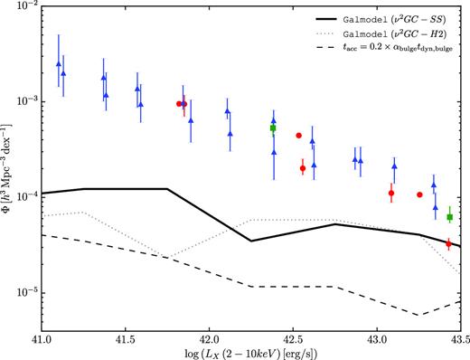
AGN LFs at z ∼ 0. To check the effect of the determination of tdyn,bulge and the accreted gas mass, we compare three models: (1) the Galmodel with the ν2GC-SS simulation (black solid line), (2) the Galmodel with the ν2GC-H2 simulation (black dotted line), and (3) the model in which tacc = 0.2 × αbulgetdyn,bulge (black dashed line). Observational results are the same as the top left panel of Fig. 5.
Another problem of the AGN LFs obtained with the ν2GC is that there are no AGNs with log (LX/erg s−1) > 45.3 at z > 2.6. Such luminous AGNs do not appear even when we employ N-body simulations with larger volumes. The modelling of the radio-mode AGN feedback is likely to be responsible for this, which was originally proposed by Bower et al. (2006) and is similar to other SA models. Host halo masses of AGNs with log (LX/erg s−1) ∼ 45.0 at z ∼ 4 in the fiducial AGN model are |$10^{12-13} \, \mathrm{M}_\odot$|. Such massive haloes could satisfy conditions of equations (22) and (23) and the gas cooling is quenched even at high redshifts. This is shown in Fig. 15, which shows the fraction of galaxies whose gas cooling is quenched by the radio-mode AGN feedback. We find that about the half of galaxies are quenched when |$M_\mathrm{halo} \gt 10^{12.5} \, \mathrm{M}_\odot$| at z ∼ 4. We will address this problem in future studies.
![The fraction of central galaxies whose gas cooling is shut off by the radio-mode AGN feedback at z ∼ 4. The x-axis is the host halo mass of the galaxies. The number means [Quenchedhalo]/[Totalhalo].](https://oup.silverchair-cdn.com/oup/backfile/Content_public/Journal/mnras/482/4/10.1093_mnras_sty2958/1/m_sty2958fig15.jpeg?Expires=1716540970&Signature=pWuRwcKRSCwEA8e1PZNgDNkpVkM6bNVZGwVaM5dTvVZXmaplSd8vCIWxHhQVBBRs0R4tIj2Qt0eV~7I7ekEh~Cvlz7tyAKaDR~ZskrKgaoBcN8rcI81JC69Sr~J6-MNBuoF-tr6os1r1092xIjur9bacHnsBNAUmavfHq2CypDDa~dg6bvORayBgAmj91w4c5a86yo5ygMq1KQprBBR56uDiekyv0WacLYDeGanNjgpUuw2lvU4ZpemEhjXAFBd~jiyMnwWTq8FFe23zVIHlcRspwAVffWh5XCm73QDjvYrvAPrUmMtEy5ATay-mDfXfsuLwC21B7zcDw~1GIrtiDg__&Key-Pair-Id=APKAIE5G5CRDK6RD3PGA)
The fraction of central galaxies whose gas cooling is shut off by the radio-mode AGN feedback at z ∼ 4. The x-axis is the host halo mass of the galaxies. The number means [Quenchedhalo]/[Totalhalo].
ACKNOWLEDGEMENTS
We appreciate the detailed review and useful suggestions by the anonymous referee, which have improved our paper. We would like to express the deepest gratitude to A. R. Pettitt for thorough English proofreading that drastically improves the paper. We thank J. Aird to give the fitting function of hard X-ray luminosity functions of AGNs. We appreciate the fruitful comments from the observational side by T. Izumi, M. Onoue, Y. Ueda, D. Zhao, T. Nagao, Y. Matsuoka, Y. Kimura, and M. Akiyama. We also thank K. Wada for theoretical comments. HS has been supported by the Sasakawa Scientific Research Grant from The Japan Science Society (29-214) and Japan Society for the Promotion of Science (JSPS) KAKENHI (18J12081). TO has been financially supported by the Ministry of Education, Culture, Sports, Science and Technology (MEXT) KAKENHI (16H01085). TK was supported in part by an University Research Support Grant from the National Astronomical Observatory of Jpan (NAOJ) and JSPS KAKENHI (17K05389). MN has been supported by the Grant-in-Aid (25287041 and 17H02867) from the MEXT of Japan. TI and TO have been supported by MEXT as ‘Priority Issue on Post-K computer’ (Elucidation of the Fundamental Laws and Evolution of the Universe) JICFuS. TI has been supported JSPS KAKENHI Grant Number 15K12031. RM was supported in part by MEXT KAKENHI (15H05896). TO was supported by World Premier International Research Center Initiative (WPI). KO has been supported by JSPS KAKENHI (16K05299).
Footnotes
Even when we consider AGNs triggered only by major mergers, the ‘anti-hierarchical trend’ of optical QSOs (i.e. luminous AGNs) can be explained (Enoki et al. 2014).
Cosmological simulation data are available from the following link: http://hpc.imit.chiba-u.jp/∼ishiymtm/db.html.
We assume that gas and stars in the disc have the same scale radius (see, however, Mitchell et al. 2018).
This also corresponds to the star formation time-scale for a starburst (Nagashima et al. 2005).
Mej in Lacey et al. (2016) is the same as Mreheat in ν2GC although both are calculated with the same procedure.
Mreheat is given as Mhot in M16.
M16 assume that only major mergers are induced starbursts in bulges and a galactic disc is completely destroyed by a major merger while it does not change by a minor merger.
Since the stellar mass difference between Chabrier and Kroupa IMF is only ∼ 0.04 dex (Muzzin et al. 2013), we assume a negligible difference in our results.
REFERENCES
APPENDIX A: GALAXY MODELLINGS
A1 Gas cooling
Here, we describe the calculation of the amount of the cold gas, which is accreted on to a central galaxy. In the model, we define a central galaxy of a new common halo as the central galaxy of the most massive progenitor halo.
We note that we assume the existence of a ‘cooling hole’ in the same way as M16. Since we assume that the radial profile of the remaining hot gas is unchanged until the DM halo mass doubles, there is no hot gas at r < rcool once the gas cools and is accreted on to the central galaxy.
A2 Star formation
Our model includes star formation in cold gas discs and reheating of the gas by SNe. The implementation is similar to that of M16.
The gas reheated by SNe would not be available for gas cooling immediately. We do not severely differentiate the ejected and reheated gas by SNe. In our model, the gas with mass βMreheat cannot cool immediately and is stored in a reservoir due to the reheating and ejection by SNe. A fraction of this gas might return to the hot gas halo and cool with some time-scale. Lacey et al. (2016) assume the returned gas mass as αreturn Mej,7 where αreturn is a free parameter. We, however, simply assume that αreturn = 0 and that all of the reheated gas falls back to the halo as hot gas when the halo mass doubles without escaping from the halo. If we set αreturn = 1.0, the cosmic star formation density at z < 1.0 becomes only ∼1.3 times larger.
A3 Size of galaxies
Here, we describe how to estimate galaxy size, the circular velocity of galactic discs, and the velocity dispersion of bulges.
A3.1 Disc size and circular velocity
We assume that DM and hot gas haloes have the same specific angular momentum and that the angular momentum is conserved during the formation of a cold gas disc. We adopt the lognormal distribution for the dimensionless spin parameter, λH ≡ L|E|1/2/GM5/2, where L, E, and M are the angular momentum, binding energy, and DM halo mass, respectively, the same prescription as M16. The mean value of λH is 0.042 and the logarithmic variance is 0.26, which are obtained from N-body simulations of Bett et al. (2007).
We note that Rd becomes smaller than that at the previous time-step when a merger of galaxies or disc instability occurs, by which the disc mass of the primary galaxy decreases. We then consider the conservation of the angular momentum and set the new effective radius, Rd,new, as Rd,new = (M0d/M1d) × Rd, where M0d and M1d are the disc mass (stellar + cold gas) of the primary galaxy after and before the merger or disc instability, respectively.
A3.2 Bulge size and velocity dispersion
We describe how to estimate bulge size and velocity dispersion when a merger of galaxies or a disc instability occurs. There have been several previous studies (e.g. Hopkins et al. 2009b; Covington et al. 2011; Shankar et al. 2013) which investigate how to calculate the size and velocity dispersion of the bulge from the Virial theorem and energy conservation. They, however, only study the major merger case. Applying their result to galaxies experiencing minor mergers or a disc instability, by which a galactic disc is not completely destroyed, is not straightforward. In this paper, we apply the similar formula to M169 to obtain size and velocity dispersion of bulges formed not only by major mergers but also by minor mergers and disc instability.
For the disc instability, we employ the same formulae as those for the merger of galaxies while subscripts, i = {1, 2}, indicate the bulge and disc, respectively and the orbital energy, Eorb, is set to be 0.
A3.3 Dynamical response caused by SNe feedback
We consider the change of the size and velocity caused by SN feedback. The SN feedback continuously expels gas from a galaxy. As a result, the gravitational potential well becomes shallower and the gravitationally bound system expands and its rotation speed slows down (Yoshii & Arimoto 1987). We refer to this effect as dynamical response, which is taken into account the same way as M16. This affects the size of galactic discs and bulges, the rotation velocity of galactic discs and their host haloes, and the velocity dispersion of galactic bulges. See section 2.8 of M16 for farther details.
A4 Photometric properties and morphological identification
The morphological types of model galaxies are determined in the same manner as M16; using bulge-to-total (B/T) luminosity ratio in Bband, galaxies with B/T > 0.6, 0.4 < B/T < 0.6, and B/T < 0.4 are classified as elliptical, lenticular, and spiral galaxies, respectively (Simien & de Vaucouleurs 1986).
APPENDIX B: GENERAL RESULTS OF GALAXIES
In this section, we present properties of galaxies obtained from the fiducial model and compare them with those obtained from observations. First, we run the MCMC fitting with the ν2GC-SS simulation to tune parameters. For the model calibration, we use observed K- and r-band LFs at z ∼ 0 obtained from the Galaxy and Mass Assembly (GAMA) survey, H i mass function at z ∼ 0 extracted from the data of the Arecibo Legacy Fast ALFA (ALFALFA) survey, MBH–Mbulge relation at z ∼ 0 (equation 11 Kormendy & Ho 2013), scaling relations of galactic discs and bulges at z ∼ 0 (Courteau et al. 2007; Forbes et al. 2008, respectively) cosmic SFR density obtained from observations (UV and IR bands, and radio 1.4 GHz), K-band LFs at z = 1, 2, 3 obtained with the UKIDSS Deep Survey (Cirasuolo et al. 2010), and AGN hard X-ray LFs at z = 0.4, 1, 2 (Ueda et al. 2014).
We summarized the fiducial values of our free parameters and related equations in Table B1. We run the calculation with 50 000 realizations, excluding the initial 10 000 steps of the ‘burn-in’ phase (for more details, see Section 3.2 in Makiya et al. 2016). The reduced χ2 decreases at 3.4 per cent of the initial value after the first 10 000 iterations, and at 1.5 per cent after 20 000 iterations. After 20 000 iterations, χ2 becomes a little larger (2.2 per cent/2.3 per cent of the initial value after 40 000/50 000 iterations). The dispersion of values of MCMC-fitted parameters after 50 000 iterations is 1.69/1.29 times larger than that after 20 000/40 000 iterations. The averaged values of parameters, on the other hand, seems to be converged. The change of the averaged values of parameters is 4.7 per cent from 20 000 to 50 000 iterations and 1.4 per cent from 40 000 to 50 000 iterations. The increase of the iterations would thus cause the increase of the dispersion values.
Summary of free parameters in the fiducial model. Almost all parameters are fitted with the MCMC method (iteration = 50 000). We show the (1) parameter name, (2) related equation or section, (3–5) parameter range, best-fitting value, and dispersion (if MCMC fitted parameter), and (6) adopted value.
| Parameter | Related equation | Value range | MCMC best | MCMC dispersion | Adopted value |
|---|---|---|---|---|---|
| Galaxies | |||||
| αstar | Equation (A8) | [−3.0, 0.0] | −2.14 | 0.10 | −2.14 |
| Vstar (km s−1) | Equation (A8) | [100.0, 400.0] | 211.30 | 14.37 | 197.00 |
| εstar | Equation (A8) | [0.05, 0.50] | 0.48 | 0.02 | 0.46 |
| Vhot (km s−1) | Equation (A10) | [50.0, 400.0] | 121.64 | 2.74 | 121.64 |
| αhot | Equation (A10) | [0.0, 4.0] | 3.92 | 0.07 | 3.92 |
| αreturn | Section A2 | 0.00 | |||
| fmrg | Section 2.1.1 | [0.8, 1.0] | 0.98 | 0.01 | 0.81 |
| fmajor | Section 2.1.1 | [0.3, 1.0] | 0.89 | 0.08 | 0.89 |
| κdiss | Equation (A23) | [1.0, 3.0] | 2.70 | 0.20 | 2.75 |
| |$M_\mathrm{h0} \,(10^{14} \, \mathrm{M}_\odot )$| | Equation (A19) | [0.1, 10.0] | 2.10 | 1.43 | 1.00 |
| αh | Equation (A19) | [0.5, 2.0] | 1.82 | 0.13 | 1.82 |
| εDI,crit | Equation (5) | [0.7, 1.1] | 1.05 | 0.01 | 0.75 |
| fbar | Section 2.1.2 | [1e−3, 1.0] | 0.63 | 0.10 | 0.63 |
| τV0 | Section A4 | 2.5 × 10⁻⁹ | |||
| SMBHs and AGNs | |||||
| αcool | Equation (23) | [0.8, 1.2] | 1.14 | 0.04 | 1.14 |
| log (εSMBH) | Equation (24) | [−3.0, 0.0] | −2.66 | 0.53 | −2.66 |
| fBH | Equation (A12) | [1e−3, 8e−2] | 0.06 | 0.01 | 0.02 |
| |$M_\mathrm{seed} \, (\mathrm{M}_\odot )$| | Section 2.2.1 | 103 | |||
| αbulge | Equation (15) | [0.1, 1.2] | 0.77 | 0.24 | 0.58 |
| τloss,0 (Gyr) | Equation (16) | [0.1, 5.0] | 1.56 | 0.71 | 1.00 |
| γgas | Equation (16) | [−5.0, 0.0] | −3.28 | 0.41 | −4.0 |
| γBH | Equation (16) | [0.0, 5.0] | 4.40 | 0.42 | 3.5 |
| |$\skew4\dot{m}_\mathrm{crit}$| | Equation (17) | 10.0 | |||
We have checked the correlations between values of two different parameters by using the Pearson’s r (Table B2). The correlation is weak for most combinations of two parameters although some (αstar–Vstar, κdiss–εSMBH, Mh0–αbulge, Mh0–tloss,0, αbulge–tloss,0, and γgas–γBH) have strong correlations, |r| ≳ 0.8.
List of the Pearson’s r.
| γBH | γgas | αbulge | τloss,0 | fBH | fbar | εDI,crit | log (εSMBH) | αcool | αh | Mh0 | κdiss | fmajor | fmrg | αreturn | αhot | Vhot | εstar | Vstar | |
|---|---|---|---|---|---|---|---|---|---|---|---|---|---|---|---|---|---|---|---|
| αstar | −0.25 | 0.19 | 0.39 | 0.34 | 0.08 | −0.16 | 0.06 | 0.31 | −0.30 | 0.19 | −0.34 | −0.08 | 0.21 | 0.48 | −0.17 | 0.05 | −0.30 | 0.05 | 0.80 |
| Vstar | −0.27 | 0.23 | 0.54 | 0.42 | 0.20 | −0.13 | −0.25 | 0.39 | −0.37 | 0.12 | −0.46 | −0.21 | 0.28 | 0.51 | −0.12 | 0.20 | −0.02 | 0.44 | |
| εstar | −0.02 | 0.10 | 0.31 | 0.27 | 0.38 | −0.22 | −0.09 | 0.16 | −0.18 | 0.11 | −0.32 | −0.20 | 0.26 | 0.17 | 0.13 | 0.20 | −0.05 | ||
| Vhot | 0.22 | −0.25 | −0.20 | −0.29 | −0.36 | 0.33 | −0.74 | −0.21 | 0.16 | −0.47 | 0.23 | 0.12 | −0.35 | −0.08 | 0.08 | −0.62 | |||
| αhot | −0.24 | 0.25 | 0.38 | 0.36 | 0.48 | −0.31 | 0.29 | 0.26 | −0.24 | 0.39 | −0.33 | −0.24 | 0.42 | 0.15 | −0.07 | ||||
| αreturn | −0.06 | 0.07 | −0.17 | −0.26 | −0.25 | 0.07 | −0.09 | −0.03 | 0.39 | −0.03 | 0.35 | 0.14 | −0.45 | −0.19 | |||||
| fmrg | 0.23 | −0.24 | 0.27 | 0.22 | 0.18 | −0.29 | −0.12 | 0.04 | −0.29 | −0.11 | −0.38 | 0.08 | 0.24 | ||||||
| fmajor | −0.38 | 0.41 | 0.62 | 0.69 | 0.75 | −0.47 | 0.18 | 0.23 | −0.33 | 0.57 | −0.71 | −0.20 | |||||||
| κdiss | 0.52 | −0.59 | −0.70 | −0.71 | −0.52 | −0.28 | −0.24 | −0.80 | 0.69 | −0.36 | 0.49 | ||||||||
| Mh0 | 0.29 | −0.36 | −0.82 | −0.89 | −0.79 | 0.16 | −0.17 | −0.45 | 0.73 | −0.42 | |||||||||
| αh | −0.57 | 0.61 | 0.54 | 0.59 | 0.64 | −0.50 | 0.34 | 0.46 | −0.32 | ||||||||||
| αcool | 0.13 | −0.19 | −0.74 | −0.70 | −0.67 | 0.02 | −0.19 | −0.60 | |||||||||||
| log (εSMBH) | −0.61 | 0.67 | 0.72 | 0.68 | 0.42 | 0.10 | 0.23 | ||||||||||||
| εDI,crit | −0.18 | 0.21 | 0.12 | 0.26 | 0.27 | 0.07 | |||||||||||||
| fbar | −0.02 | 0.02 | −0.14 | −0.11 | −0.36 | ||||||||||||||
| fBH | −0.26 | 0.38 | 0.74 | 0.79 | |||||||||||||||
| αbulge | −0.59 | 0.66 | 0.91 | ||||||||||||||||
| τloss,0 | −0.57 | 0.61 | |||||||||||||||||
| γgas | −0.94 |
The MCMC fitting has two crucial problems. First, since the ν2GC-SS simulation has only 703h−3Mpc3, we cannot fit the bright end slope of AGN LFs. The larger box simulations are not realistic considering the computational cost. Secondly, we have to fit parameter values so that all observational results are equally well reproduced. In other words, we cannot prioritize observational properties to fit. We therefore use the ν2GC-SS simulation and refit some ill-fitted parameters by hand so that they are in 1σ in the MCMC-fitted values. The parameters which are refitted by hand are shown in Table B1. We cannot determine the values of fmrg, εDI,crit, fBH, γgas, and γBH because of the degeneracy and the small box size.
The main results of this paper on the statistical properties of SMBHs and AGNs appear in Section 3. Additional properties of galaxies such as size/velocity–magnitude relations of galactic discs, stellar mass–SFR relations appear in Appendix B2.
B1 Properties of galaxies at z ∼ 0
Fig. B1 shows the K- and r-band LFs at z ∼ 0. The results of the fiducial model with the ν2GC-SS and -H2 simulations shown to test the resolution effect. We overplot the results obtained by M16 in grey dash–dotted lines. Red points with errorbars are the observational estimates by the GAMA survey (Driver et al. 2012). Fig. B2 shows the H i mass function (MF) at z ∼ 0. We assume the relation between the cold gas mass and the atomic hydrogen gas mass, MH i, as MH i = 0.54Mcold, which is the same relation used in M16.
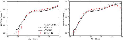
K- and r-band LFs of galaxies. Black dashed and solid lines show the results by the fiducial model with ν2GC -SS and ν2GC -H2 simulations, respectively. We show the result of M16 as grey dot–dashed lines. Red filled circles with error bars are observational estimates by the GAMA survey (Driver et al. 2012).
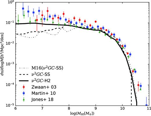
H i MF at z ∼ 0. Black dashed and solid lines show the results obtained from the fiducial model with ν2GC-SS and ν2GC-H2 simulations, respectively. We show the result of M16 as grey dot–dashed lines. Red filled circles, blue filled squares, and green filled triangles with error bars are observational data obtained from the HIPASS (Zwaan et al. 2003) and ALFALFA surveys (Martin et al. 2010; Jones et al. 2018), respectively.
The bright-end slopes of the LFs and the massive-end slope of the H i MF are sensitive to the values of αcool and εSMBH, which are both related to the radio-mode AGN feedback. The faint-end slopes are determined by the energy of the SN feedback determined by αhot and Vhot. The low-mass end slope of the H i MF is also sensitive to the values of αstar and Vstar, which determine the gas consumption time-scale by star formation. Although the model explains the wide range of the observed LFs and H i MF at z ∼ 0, the number of galaxies with smaller H i gas mass (|$M_\mathrm{H\,{\small{I}}} \lt 10^8 \, \mathrm{M}_\odot$|) is underpredicted, which is the same trend as M16 and other SA models (e.g. Gonzalez-Perez et al. 2014; Lagos et al. 2014; Lacey et al. 2016). This is partly due to the insufficient resolution of the employed N-body simulation. As shown in Fig. B2, the result with the ν2GC-H2 simulation (∼43 times higher mass resolution than the ν2GC-SS simulation) explains the H i MF better than that with the ν2GC-SS simulation and the result is nearly consistent with the recent observational estimates (Jones et al. 2018, green triangles) The modelling of the SFR might be important since the low-mass end slope is sensitive to αstar and Vstar. The modelling of the gas stripping and cooling of satellite galaxies should also be important. However, we do not use sub-halo merger trees in this work, and do not consider gas cooling for satellite galaxies. Since such less massive galaxies do not have an impact on the main results of this paper, we leave this issue for future work.
We compare the predicted effective radius and rotation velocity of spiral galaxies at z ∼ 0 with observations. We employ the ν2GC-SS ν2GC-H2 simulations to obtain the result. We use the data obtained from Courteau et al. (2007), who estimated the disc scale lengths from I-band image and the disc rotation velocities from H α or H i line width. Figs B3 and B4 are the scaling relations between the rotation velocity and the I-band magnitude (the so-called Tully–Fisher relation; Tully & Fisher 1977) and the effective radius and the I-band magnitude, respectively. The data obtained from Courteau et al. (2007) are presented as red points. The results of their model are shown as black lines with error bars which are the 10th to 90th percentiles. The model results are consistent with the observational results and the effect of the mass resolution of the simulations is negligible.
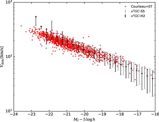
Rotation velocities of spiral galaxies as a function of I-band magnitude (Tully–Fisher relation). The black line shows the median value obtained by the model and the error bars show the 10th and 90th percentiles from the ν2GC-SS ν2GC-H2 simulations. Red points show the observational data obtained from Courteau et al. (2007).
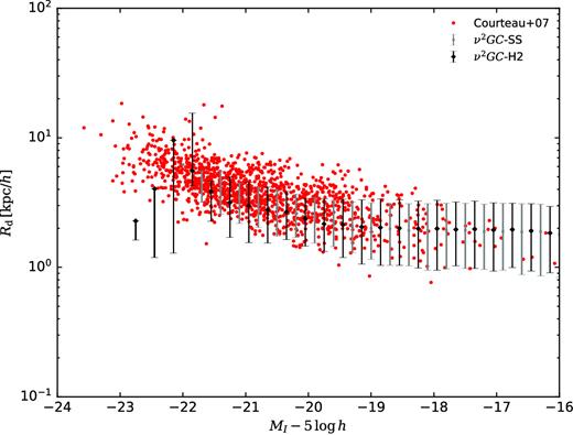
Effective radius of spiral galaxies as a function of I-band magnitude. The black line shows the median value obtained by the model and the error bars show the 10th and 90th percentiles. We employ the ν2GC-SS ν2GC-H2 simulations. Red points show the observational data obtained from Courteau et al. (2007). We convert the scale length obtained by Courteau et al. (2007) to the effective radius with Rd = 1.68rds.
Next, we compare the predicted effective radius and velocity dispersion of elliptical and S0 galaxies at z ∼ 0 with observations since these values are used for calculating the dynamical time of bulges. Here, we also employ the ν2GC-SS and ν2GC-H2 simulations, although the effect of the mass resolution of the simulations is negligible. We use the data obtained from Forbes et al. (2008), who calculate the half-light radii are from 2MASS K-band 20th isophotal by using an empirical relation based on Sérsic light profiles (Forbes et al. 2008). Figs B5 and B6 are the scaling relations between the bulge velocity dispersion and the K-band magnitude (the so-called Faber–Jackson relation; Faber & Jackson 1976) and the effective radius and the K-band magnitude, respectively. The data obtained from Forbes et al. (2008) are shown in red points. The results of the fiducial model with ν2GC-SS/-H2 are described as grey squares/black diamonds with error bars indicating 10th and 90th percentiles. For comparison, we overplot the model results with MDM,1 = 0 as grey diamonds with error bars. We find that the effective radius of bulges with MK − 5log h < −23 becomes smaller when we set MDM,1 = 0. The results obtained from the fiducial model have some discrepancies with the observational results, especially for the velocity dispersion while the bulge MF at z ∼ 0 is consistent with observed bulge MF obtained from Moffett et al. (2016), and Thanjavur et al. (2016), as shown in Fig. B7.
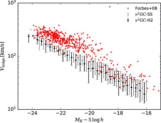
Velocity dispersions of elliptical and S0 galaxies as a function of K-band magnitude (Faber–Jackson relation). The black line shows the median value obtained by the model and the error bars show the 10th and 90th percentiles from the ν2GC-SS and ν2GC-H2 simulations. Red points show the observational data obtained from Forbes et al. (2008).
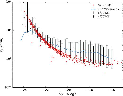
Effective radius of elliptical and S0 galaxies as a function of K-band magnitude. The black line shows the median value obtained by the model and the error bars show the 10th and 90th percentiles. The grey line with errorbars shows the median value obtained by the model considering MDM,1 = 0 from the ν2GC-SS and ν2GC-H2 simulations. Red points show the observational data obtained from Forbes et al. (2008).
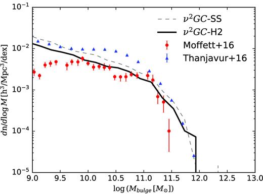
The velocity dispersion obtained from the fiducial model becomes smaller with massive galaxies than those obtained from observations. There might be two possible reason for the inconsistency. First, due to the underestimate of gas mass especially in the small galaxies. We find that the model overproduces gas-poor galaxies, whose r-band magnitude are less than ∼−18.5. The dissipation process plays important roles for calculation of the velocity dispersion (Section A3.2). Since the dissipated energy becomes larger with mergers of more gas-rich galaxies, underestimation of the cold gas mass would cause the underestimation of the velocity dispersion. Another possibility to reproduce Faber–Jackson relation might be related with the estimation of the gravitational potential of galactic discs. Galaxies which experience bulge growths should contain a galactic disc. The potential energy of the remained disc is estimated assuming that the rotation velocity of the disc remain unchanged (equation A20). When the discs have a shallower potential, the bulge should display a larger velocity dispersion.
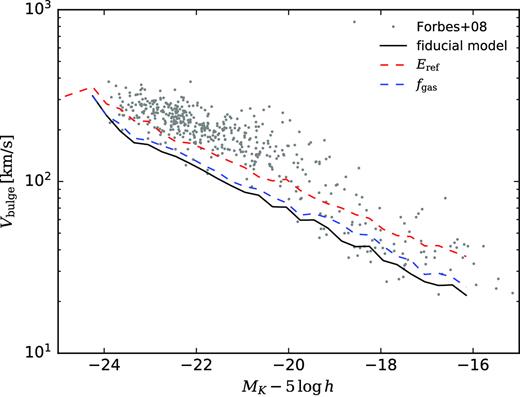
Velocity dispersions of elliptical and S0 galaxies as a function of K-band magnitude (Faber–Jackson relation). The black solid, red dashed, and blue dashed lines show the median value obtained by the fiducial model (ν2GC-SS), that by the artificially fixed gas fraction (equation B1), and that by the artificially fixed energy which remains in the galactic disc, respectively. Grey points show the observational data obtained from Forbes et al. (2008).
B2 Galaxy evolution
We first show the cosmic SFR density as a function of redshift in Fig. B9. The black solid line is the model result obtained with the ν2GC-SS simulation and points are the results obtained from observations in IR bands (Pascale et al. 2009; Rodighiero et al. 2010), radio 1.4 GHz (Karim et al. 2011), UV bands (Cucciati et al. 2012; Bouwens et al. 2014; Ouchi et al. 2004), and a compilation of various observations (Hopkins 2004, and therein). We find that the cosmic SFR density obtained by the fiducial model is consistent with the data over wide redshift range.
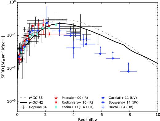
Cosmic SFR density as a function of redshift. The black solid line is the model results obtained with the ν2GC-SS and ν2GC-H2 simulations. Red filled triangles and stars and cyan filled squares are obtained from dust continuum emission (Pascale et al. 2009; Rodighiero et al. 2010; Karim et al. 2011, respectively). Blue stars, filled circles, and filled diamonds are from UV continuum emission (Ouchi et al. 2004; Cucciati et al. 2012; Bouwens et al. 2014, respectively). Black crosses are obtained from Hopkins (2004), which is a compilation of various other observational results.
Next, we present the evolution of K- and B-band LFs and stellar MFs of galaxies obtained by the fiducial model with the ν2GC-M and -H2 simulations to show the result of bright and rare populations of galaxies. The LFs and MFs presented here are volume-weighted. The details of the calculation of LFs and MFs from the simulation are described in Appendix D.
Fig. B10 shows the model K-band LFs (black solid lines) compared with observational results (Bell et al. 2003; Drory et al. 2003; Huang et al. 2003; Pozzetti et al. 2003; Caputi et al. 2006; Saracco et al. 2006; Devereux et al. 2009; Cirasuolo et al. 2010; Driver et al. 2012). Model LFs reproduce observational results well for z < 3.5 including faint-end slopes. The model of M16 also explains observed K-band LFs for z < 2.0 well (figure 21 of M16), although it over estimates number density of less luminous galaxies (MK > −22).
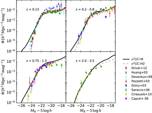
K-band LFs of galaxies at z < 0.13, z = 0.2–0.8, z = 0.75–1.3, and z = 2.0–3.5. The model LFs (volume-weighted) by the ν2GC-M simulation appear as black solid lines. Observational estimates are taken from Bell et al. (2003), Huang et al. (2003), Pozzetti et al. (2003), Drory et al. (2003), Caputi et al. (2006), Saracco et al. (2006), Devereux et al. (2009), Cirasuolo et al. (2010), and Driver et al. (2012).
Fig. B11 compares the model B-band LFs (black lines) with observational results (Norberg et al. 2002; Gabasch et al. 2004; Giallongo et al. 2005; Ilbert et al. 2005; Jones et al. 2006). The dust attenuated model LFs are shown by the solid lines (for dust correction, see Section A4) and LFs without dust attenuation are shown by the dashed lines. We note that the data obtained from Norberg et al. (2002) and Jones et al. (2006) at z < 0.25 are not dust attenuation corrected. Therefore, their results allow a fair comparison with the LF of the dust attenuated model. The dust attenuation corrected model LFs at z > 0.8 seem to be inconsistent with observational estimates. The observational data of Giallongo et al. (2005) are dust attenuation corrected by assuming SMC and Calzetti extinction curves. Considering the correction for the dust attenuation, the model reproduces observed B-band LFs at z < 3.5 reasonably well. The data of Ilbert et al. (2005) and Gabasch et al. (2004) are not dust attenuation corrected. Since the bright-end of LFs of Giallongo et al. (2005), Ilbert et al. (2005), and Gabasch et al. (2004) are similar and the dust attenuation in B band should have less impact than those suggested from the fiducial model, we conclude that some modifications of the dust attenuation are needed, which we leave for future studies.
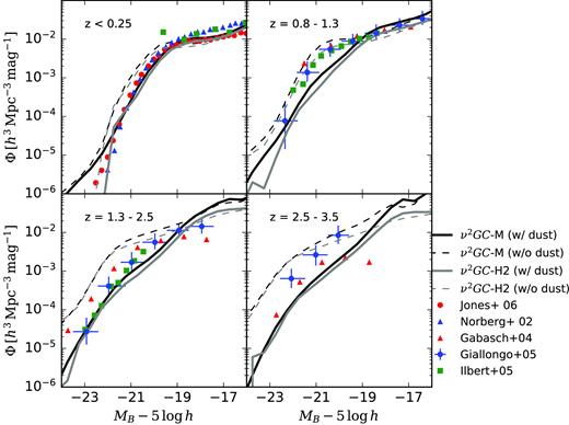
B-band LFs of galaxies at z < 0.25, z = 0.8–1.3, z = 1.3–2.5, and 2.5–3.5. The model LFs (volume-weighted) obtained with the ν2GC-M and -H2 simulations appear in black solid and grey dashed lines (with dust attenuation) and black dashed lines (without dust attenuation). Observational results are obtained from Norberg et al. (2002), Gabasch et al. (2004), Ilbert et al. (2005), Giallongo et al. (2005), and Jones et al. (2006).
Fig. B12 shows the stellar MFs from z ∼ 0 to z ∼ 4.5. We adopt Chabrier IMF (Chabrier 2003) as described in Section A2. We compare our results (black lines) with observational estimates by Li & White (2009), Baldry et al. (2012), Santini et al. (2012), Muzzin et al. (2013), Moustakas et al. (2013), and Tomczak et al. (2014), who employ either a Chabrier IMF (Chabrier 2003) or Kroupa IMF (Kroupa 2001).10 While the model can reproduce the massive end of the stellar MFs at z < 3.5, we find that the model underestimates the number of massive galaxies at z > 3.5 (bottom right panel). This similar feature is seen in other SA models (e.g. Hirschmann et al. 2012; Lacey et al. 2016). The derivation of stellar masses from observations is commonly performed by the broad-band SED fitting with galaxy templates assuming a single dust attenuation law. Alternatively, Mitchell et al. (2013) suggest that the discrepancy between SA models and observations in the stellar MFs at high redshifts stems from the uncertainties in the dust attenuation curve. For less massive galaxies, we also find that we overproduce their number density at 0.4 < z < 2.5, which is the similar trend to other SA models (e.g. Weinmann et al. 2012). Some previous studies with SA models investigate this problem. Henriques et al. (2013) show that the ejected gas should be reincorporated into the system on a time-scale which depends on the halo mass; the smaller halo should have the larger time-scale, and the gas returns to the system more slowly. The importance of the time-scale to reproduce SMFs are also proposed by White, Somerville & Ferguson (2015). They also suggest the mass-loading factor which strongly depends on the redshift also plays a role in reproducing SMFs. White et al. (2015) imply a detailed comparison with observations are required to differentiate these two effects. Hirschmann, De Lucia & Fontanot (2016) consider the decrease of the gas infall rate by ‘pre-heating’ and find that their model can reproduce not only the low-mass end of SMFs but also the metal enrichment of galaxies. We need to consider such effects in the ν2GC, which we leave it for future studies to decrease of the degree of freedom. As White et al. (2015) suggest, the values of parameters which are required for reproducing SMFs strongly depends on the treatment of the reservoir of reheated and/or ejected gas in each SA models. The value of these parameters therefore have almost no constraints now.
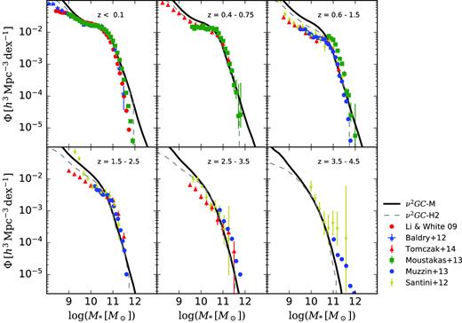
Stellar MFs at z < 0.1, z = 0.4–0.75, z = 0.6–1.5, z = 1.5–2.5, z = 2.5–3.5, and z = 3.5–4.5. The model MFs (volume-weighted) obtained with the ν2GC-M and -H2 simulations are shown in black solid and grey dashed lines. Observational results are obtained from Li & White (2009), Baldry et al. (2012), Santini et al. (2012), Muzzin et al. (2013), Moustakas et al. (2013), and Tomczak et al. (2014).
For checking the mass resolution effect, we overplot the results with the ν2GC-H2 simulation as grey dashed lines in Figs B10–B12, although the ν2GC-H2 simulation has 83 times smaller box size than the ν2GC-M simulation. We find the effect of the resolution is negligible.
We also present the relation between total stellar mass and SFR at z < 6.0 obtained from the fiducial model with the ν2GC-M simulation and compare it with that obtained from observations (Daddi et al. 2007; Elbaz et al. 2007; Salmon et al. 2015) in Fig. B13. We select all galaxies (central + satellite) without any luminosity or surface density limitations. The result is shown as the orange density map. In addition, blue points with errorbars show the relation for luminous galaxies with MFUV < −19.0 (where MFUV is the magnitude of the GALEX FUV band) obtained by the fiducial model, which are consistent with that of Salmon et al. (2015) at z > 4.0. The galaxies obtained by the fiducial model have larger SFRs than those obtained by observations when we take the selection effect into account at z > 4. Since the M*–SFR relation obtained by Salmon et al. (2015) with |$\log (M_\mathrm{*}/\, \mathrm{M}_\odot) \gt 10.3$| has a large dispersion, the slope of the M*–SFR relation would not be strictly constrained. We note that the number of luminous galaxies obtained by the fiducial model with the ν2GC-M simulation is 135.1, 180.9, and 108.1 times larger than that of Salmon et al. (2015) at z ∼ 4, 5, and 6, respectively. The galaxies with |$\log (M_\mathrm{*}/\, \mathrm{M}_\odot) \gt 10.5$| and MFUV < −19.0 at z ∼ 2 have smaller SFR than those predicted by the observational fitting. This could be a result of the AGN feedback effect (see also Section 4). At z ∼ 2, gas cooling of most of such massive galaxies are quenched by the AGN feedback. The cold gas mass, thus, becomes smaller, resulting in lower SFRs.
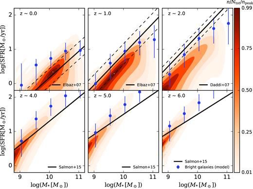
The relation between total stellar mass and SFR at z < 6.0. The model results (obtained with the ν2GC-M simulation) including all galaxies and those including only luminous galaxies (MFUV < −19.0) are shown by the orange colour map and the blue points with errorbars (10th and 90th percentiles), respectively. For comparison, we overplot the results obtained from observations at z ∼ 0 and 1 (Elbaz et al. 2007), z ∼ 2 (Daddi et al. 2007), and z ∼ 4, 5, and 6 (Salmon et al. 2015).
Izumi et al. (2018) compare this relation obtained from the fiducial model employing the ν2GC-L simulation with the data of four observed AGN host galaxies at z ∼ 6. These four AGNs, which are optically low-luminosity quasars (MUV < −25), are originally detected with Subaru Hyper Suprime Cam (HSC) (Matsuoka et al. 2017) and are observed with Atacama Large Millimeter/Submillimeter Array (ALMA) to investigate their host galaxies’ properties. They find that the sample galaxies are on or below the so-called main sequence at z ∼ 6, which are very rare population in the fiducial model of ν2GC. Luminous quasars (MUV < −25) at z ∼ 6, on the other hand, have host galaxies with higher SFR than the ‘main sequence’. The fiducial model of ν2GC can reproduce such a bursty population. As shown in fig. 8 in Izumi et al. (2018) and Fig. B13, the distribution of the SFR seems to have several sub-sequences. These sub-sequences should be artificial which result from time and mass resolution of the simulations and/or the discrete treatment of the time evolution of the hot gas density profiles and cooled gas mass. As we show in Section A1, the radial profiles of hot gas haloes remain unchanged until the DM halo mass doubles. It means that no hot gas distributes in r < rcool until the DM halo mass doubles. Since the minimum halo mass of ν2GC-M and -SS simulations is |$8.79\times 10^{9} \, \mathrm{M}_\odot$|, the radial profile of the hot gas halo of galaxies with |$M_\mathrm{*} \lt 10^9 \, \mathrm{M}_\odot$| is not updated from the formation time. A part of such galaxies therefore would contain an unphysically smaller amount of the cold gas.
APPENDIX C: THE TIME-SCALE DEPENDENCE ON BH AND ACCRETED GAS MASS
We first show that the accretion time-scale from the accretion disc to the SMBH has a negative (positive) dependence on the mass of the accreted gas (SMBH), following the viscous time-scale in the accretion discs. We classify the accretion discs by their accretion rate following Kato, Fukue & Mineshige (2008). Then, we analytically calculate the radial velocity of the gas, |vr|, and the outer radius of the accretion disc which is determined as the boundary between self-gravitating and non-self-gravitating disc, rsg. The details appear in Kawaguchi, Pierens & Huré (2004). Here, we define the Schwarzschild radius, rSch, as 2GMBH/c2, the distance from the BH normalized by rSch, |$\hat{r}$|, the viscous parameter, α, and a non-dimensional variable, |$f = 1 - \sqrt{3r_\mathrm{Sch}/r}$|. The accretion rate is simply described as ΔMacc/tvis for this calculation, where tvis is the viscous time-scale determined as tvis = rsg/|vr|. The accretion rate normalized by the Eddington mass accretion rate, |$\skew4\dot{m}$| (the Eddington mass accretion rate: LEdd/c2), is employed. The disc is classified according to the dominant opacity and pressure sources as follows.
- The outer region in which the main opacity source is (free-free) absorption and the gas is the dominant pressure source. Thenand\begin{eqnarray*} |v_\mathrm{r}| \propto \alpha ^{4/5}M_\mathrm{BH}^{-1/5}\skew4\dot{m}^{3/10}\hat{r}^{-1/4}f^{-7/10} \end{eqnarray*}We obtain |$t_\mathrm{vis}\,\propto \,M_\mathrm{BH}^{15/2}\,\Delta \,M_\mathrm{acc}^{-41/4}$|.\begin{eqnarray*} r_\mathrm{sg}/r_\mathrm{Sch} \propto \alpha ^{28/45}M_\mathrm{BH}^{-52/45}\skew4\dot{m}^{-22/45}. \end{eqnarray*}
- The middle region in which the main opacity source is electron scattering and the gas is the dominant pressure source. Thenand\begin{eqnarray*} |v_\mathrm{r}| \propto \alpha ^{4/5}M_\mathrm{BH}^{-1/5}\skew4\dot{m}^{2/5}\hat{r}^{-2/5}f^{-3/5} \end{eqnarray*}We obtain |$t_\mathrm{vis}\,\propto \,M_\mathrm{BH}^{18/5}\,\Delta \,M_\mathrm{acc}^{-22/5}$|.\begin{eqnarray*} r_\mathrm{sg}/r_\mathrm{Sch} \propto \alpha ^{14/27}M_\mathrm{BH}^{-26/27}\skew4\dot{m}^{-8/27}. \end{eqnarray*}
- The inner region in which the main opacity source is electron scattering and the radiation is the dominant pressure source. Thenand\begin{eqnarray*} |v_\mathrm{r}| \propto \alpha M_\mathrm{BH}^{0}\skew4\dot{m}^{2}\hat{r}^{-5/2}f^{1} \end{eqnarray*}We obtain |$t_\mathrm{vis}\,\propto \,M_\mathrm{BH}^{6/5}\,\Delta \,M_\mathrm{acc}^{-4/5}$|.\begin{eqnarray*} r_\mathrm{sg}/r_\mathrm{Sch} \propto \alpha ^{2/9}M_\mathrm{BH}^{-2/9}\skew4\dot{m}^{4/9}. \end{eqnarray*}
Considering these conditions, we conclude that the viscous time-scale has a positive correlation to the BH mass and negative correlation to the accreted gas mass at all radii.
Next, we consider the circumnuclear disc (CND). We consider the CND model of Kawakatu & Wada (2008), as an example, although the physical mechanisms of how the CND maintains its structure is still under discussion. In Kawakatu & Wada (2008), SNe occurred in the CND induces the tidal torque which enhances the gas accretion rate from the CND to the SMBH. When the CND becomes unstable considering from the Toomre criterion (Toomre 1964), then the star formation occurs and the accretion rate increases. Since the CND becomes stable for the massive SMBH, γBH should be positive. On the other hand, since the SFR becomes more significant for the more gas-rich galaxies, γgas should be negative. We cannot obtain constraints on the values of γBH and γgas since the model of CND is too complicated to construct a single phenomenological model of the accretion time-scale (i.e. the outer radius of the CND depends on the SMBH mass, mass density of CND itself and their host galaxy; see section 2.3 in Kawakatu & Wada 2008). With the simple assumptions (based on Kawakatu & Wada 2008), we estimate γBH ∼ −0.5 and γgas ∼ 1.0, assuming a constant star formation efficiency, constant surface densities of the host galaxy and CND, the outer radius of the CND which is proportional to |$M_\mathrm{BH}^{0.5}$|.
APPENDIX D: THE CALCULATION OF LUMINOSITY AND MASS FUNCTION
We describe the calculation of the volume-weighted LFs and MFs from the model output. We obtain LFs and MFs from the model at discrete output redshifts. On the other hand, LFs and MFs are estimated from observations in continuous redshift ranges. We thus should estimate model LFs and MFs in the same redshift ranges as observations by averaging model LFs and MFs. We will now describe the derivation of the model LFs. The calculation of MFs is the same as that of LFs, with the magnitude replaced by the logarithmic stellar mass.
APPENDIX E: THE DIFFERENCE OF OBSERVABLE FRACTION WITH HOPKINS ET AL. (2007)
The method for the estimation of the observable fraction in this paper is slightly different from that of Hopkins et al. (2007). We convert hard X-ray (2–10 keV) LFs obtained from Aird et al. (2015) to UV (1450 Å) LFs by using a bolometric correction (Marconi et al. 2004) and MUV = MB + 0.85 (Kawaguchi et al. 2001). The LFs obtained from these processes are regarded as the intrinsic UV LFs since hard X-ray (2–10 keV) LFs of Aird et al. (2015) are absorption corrected. By comparing these intrinsic UV LFs with LFs obtained from observations, we obtain the parameters of observable fractions as (A0, A1, β0, β1) = (0.16, 0.07, −0.05, 0.00) (equation 21).
We show the differences of observable fractions obtained by Hopkins et al. (2007) and by our new method in Fig. E1. The grey dotted line indicates intrinsic UV LFs and blue dashed and black solid lines show LFs considering observable fraction obtained from Hopkins et al. (2007) and this paper, respectively. We assume that the observable fraction obtained by Hopkins et al. (2007) is the same in B and UV bands. We find that in such a simple assumption, the observable fraction obtained in this paper is roughly consistent with those obtained by Hopkins et al. (2007), although they have a small (∼20 per cent, at most) difference.
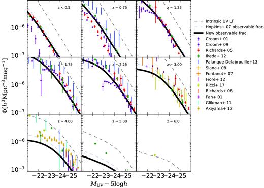
AGN LFs in UV band (1450 Å) in 0.0 < z < 6.5. Grey dashed line is the intrinsic UV LFs. Blue dashed and black solid lines are UV LFs considering observable fractions obtained from Hopkins et al. (2007) and this paper (Section 2.2.5), respectively. Observational results are obtained from Croom et al. (2001, 2009), Fan et al. (2001), Richards et al. (2005, 2006), Fontanot et al. (2007), Siana et al. (2008), Glikman et al. (2011), Fiore et al. (2012), Ikeda et al. (2012), Palanque-Delabrouille et al. (2013), Ricci et al. (2017), and Akiyama et al. (2018).
We note that UV LFs with observable fractions obtained from both Hopkins et al. (2007) and our calculation are inconsistent with observations at z > 5.0 since the fitting function of hard X-ray LFs obtained from Aird et al. (2015) can explain the observational results only at z < 5.0. We also note that the scatter of the conversion from the hard X-ray to UV luminosity are not considered for deriving the observable fraction. Akiyama et al. (2018) suggest that this scatter has significant effect on the shape of the LFs (see fig. 21 in Akiyama et al. 2018). We need to consider the effect although we leave it for future studies.
