


Abstract
Funding for substance misuse services comprises one-third of Public Health spend in England. The current allocation formula contains adjustments for actual activity, performance and need, proxied by the Standardized Mortality Ratio for under-75s (SMR < 75). Additional measures, such as deprivation, may better identify differential service need.
We developed an age-standardized and an age-stratified model (over-18s, under-18s), with the outcome of expected/actual cost at postal sector/Local Authority level. A third, person-based model incorporated predictors of costs at the individual level. Each model incorporated both needs and supply variables, with the relative effects of their inclusion assessed.
Mean estimated annual cost (2013/14) per English Local Authority area was £5 032 802 (sd: 3 951 158). Costs for drug misuse treatment represented the majority (83%) of costs. Models achieved adjusted R-squared values of 0.522 (age-standardized), 0.533 (age-stratified over-18s), 0.232 (age-stratified under-18s) and 0.470 (person-based).
Improvements can be made to the existing resource allocation formulae to better reflect population need. The person-based model permits inclusion of a range of needs variables, in addition to strong predictors of cost based on the receipt of treatment in the previous year. Adoption of this revised person-based formula for substance misuse would shift resources towards more deprived areas.
Introduction
Where local public services are funded through central government taxation, the distribution of local allocations presents a significant challenge.1 In England, the healthcare budget is split into sectors of care, each with a resource allocation formula. In 2012, public health responsibilities were transferred to Local Authorities (LA); regional bodies responsible for the delivery of a range of local services.2 There was no previous formula in place for the allocation of public health funds; a preliminary formula was generated to allocate LA public health budgets (£2.5 bn in 2013–14; 2.6% of total healthcare expenditure).3,4 The Department of Health commissioned research in 2014 to derive needs-based resource allocation formulae for drug and alcohol services (representing 31.5% of total public health expenditure), sexual health services (22.3%), and other public health services (46.2%). This paper describes the approach taken to inform the formula for drug and alcohol services.
Most healthcare systems aim to provide services based on the need for care. Reducing inequality in access and/or health has therefore become a key policy commitment.5 Distributing resources on the basis of need maximizes the efficiency of allocations.1,6 A key requirement of this approach is the ability to identify the need for healthcare. Utilization of healthcare can be used as a proxy for need, but this can be problematic, as use of services is influenced by issues of access (availability of services; patient acceptability of care; affordability). Service use, alone, may not reflect underlying need.7,8
Resource allocation formulae have been used in healthcare in England since the 1970s. Originally, geographic allocations were driven by historical expenditure. Carr-Hill et al.9 proposed utilization-based models, with costed utilization modelled against a range of potential needs measures. The resulting needs estimates informed needs indices, used to generate weighted population-based budget shares. Methodological advances have addressed the extent to which utilization data reflect access to healthcare, rather than need for healthcare. Later developments introduced regional-level indicators to control for differences in supply (access) and non-need variables to control for differentially met need (‘unmet need’).10 Subsequent refinements proposed one-stage stratified models, allowing the effects of need variables to vary across age categories and for the effects of age to be estimated, conditional on variation in supply.11 More recently, person-based allocation methods, preferred where appropriate data are available, have been used for acute hospital12 and mental health services.13
The current substance misuse resource allocation formula3 is based on actual activity (76% weighting in 2014–15), need (proxied by the Standardized Mortality Ratio (SMR) in under 75 year olds; 24% weighting), and performance (20% weighting in 2013–14, 0% after). Treatment activity figures are partitioned into opiate and/or crack cocaine users (OCU) and non-OCUs. This may be improved as follows: SMR is a narrow measure of need—other factors, e.g. deprivation, may better identify need for drug and alcohol services; supply-side and unmet-need biases were not accounted for; and analyses were conducted at an aggregate level. We aimed to develop needs-based formulae for distributing resources for substance misuse services. This entailed:
Expanding measures of need.
Accounting for supply-side influences on service use.
Estimating relative need using person-level data.
Methods
Data sources
Utilization data were sourced from the National Drug Treatment Monitoring System (NDTMS). NDTMS routinely collects data on the use of structured community-based or residential treatment for drug or alcohol misuse in England. The most recent available data (2013/14) were used, relating to c. 319 000 individuals engaging in c. 413 000 treatment episodes. Area of residence was defined by the combination of postcode sector and Local Authority (LA), creating the most granular area of residence available within this dataset (n = 10 039 areas). Multiple areas were created where more than one sector was contained within a LA or where sector and LA were not coterminous. Mid-year population estimates by age, sex and postcode were obtained from the Office for National Statistics (ONS) and converted into the Post Sector/LA level areas.
A literature search informed potential needs variables. Drug treatment clients are characterized by male gender, white ethnicity, involvement in crime, poor mental and physical health, unstable accommodation, unemployment, receipt of welfare benefits and previous drug treatment episodes.14–16 Drug and alcohol misuse in the community has been associated with additional factors, including population density,17 urbanicity,18 neighbourhood instability,19 homelessness,20 low socioeconomic status,18 disadvantaged background,21 poor school performance,21 teenage pregnancy22 and single parenting.18 These were sourced from area-level 2011 Census data, Index of Multiple Deprivation (IMD 2010) and Neighbourhood Statistics and included the following rates: benefit claimants; lone parents; unemployment; 16+ population with no qualifications; population turnover; under-18 conceptions; and homelessness, in addition to SMR, ethnicity, average household size and indicators of population density. Data were required to be readily available, routinely updated and statistically robust with coverage across England.
The needs of young people attending substance misuse services can differ from those of adult clients. In particular, young people are more likely to present with problematic cannabis use than adult clients, which may be associated with different predictors. Younger people are also less likely than adults to present with problematic use of alcohol.23
Where data points were missing because of changes to geographical output areas, 2011 area data were calculated using ONS best-fit lookup tables.24 Remaining missing data points were calculated using the mean score of neighbouring areas. LSOA-, MSOA- (middle-layer super output area, n = 6791) and LA-level (n = 151) predictor variables were mapped into post sector/LA areas by weighting on postcode populations.
Supply variables (extracted from NDTMS) included mean waiting times, the distance (km) from post sector centroid to postcode of the nearest drug treatment service, and the proportion of substitute prescribing accounted for by GPs. As a source of prescribing not sourced via public health budgets, the latter measure acted as a proxy of additional capacity and treatment choice.
Costs
Average costs per day of individual structured drug and alcohol interventions were obtained from Public Health England (PHE). Costs were derived from a 2008/09 survey of treatment agencies (PHE unpublished data) to which inflationary uplifts were applied. Total costs, accounted for by NDTMS-recorded interventions, in 2013/14 were £920 million.
Costs which could not be assigned to an area (5% of total), as client area of residence was not recorded, were assigned geographically, according to the distribution of known cases. Where postcode sector was not recorded, costs were redistributed within the LA, weighted by known treatment costs by age group within that LA. Where LA was missing, costs were redistributed nationally, weighted by known treatment costs by age group nationally.
Analysis
Our analytical approach was to replicate approaches that have been used previously for other elements of health funding in England. Three approaches have been used: (i) age-standardized models, (ii) age stratified models and (iii) person-based models.
A series of models used both needs and supply variables to predict area-level cost of substance misuse service provision. The inclusion of supply measures reduces confounding on the needs estimates where correlations exist between the supply and needs measures, and supply and costed use.
A series of stepwise regressions determined inclusion of needs variables in the final models with the order of inclusion determined by the relative coefficient size of associations between covariate z-scores and the dependent variable. Covariates with a high degree of collinearity with other variables (VIF > 5) were removed. The resulting covariate set was entered into linear regression models, accounting for Upper Tier Local Authority (UTLA), the administrative area responsible for commissioning drug and alcohol treatment provision.
The coefficients of the needs variables were used to generate the needs index. This adds needs-specific ‘weights’ to areas at the commissioning level (UTLA). The inclusion of supply measures in the regression analysis but exclusion in the needs index serves to ‘sterilize’ the formula from reflecting supply-side access bias due to the removal of observable supply-side confounding on the needs estimates.25
Analyses used SPSS version 20 and STATA version 13.
Model 1: age-standardized model
A model was developed to examine predictors of small-area variation in the age-standardized ratio of actual cost to expected cost (1-year period). This was the approach used prior to the CARAN (Combining Age Related and Additional Needs) review.9 Areas with a small population size (n < 30, 7%, n = 673) were excluded to avoid undue leverage on the model by extreme cost ratio values. Expected cost was obtained by calculating national cost per capita for eight age bands (<15, 15–19, 20–24, 25–29, 30–44, 60–64, 65+) and applying these costs to each area, using age-specific 2011 population data. Analyses were weighted by expected costs for each area. Since the need for drug services and alcohol services may differ we estimated three models: all service use, drug services only and alcohol services only.
Model 2: age-stratified model
Model 1 assumes the effects of the needs measures are the same across all age groups. Model 2 relaxes this assumption by analysing predictors of small-area variation in the ratio of actual to expected cost separately for different age groups. This was the econometric approach taken in both the CARAN and the RAMP (Resource Allocation for Mental health and Prescribing) review.26 Younger clients in treatment may differ from over-18s. Separate analyses were therefore performed for over-18s and under-18s. Areas with small (n < 30) adult (18+) populations (n = 760) and under-18 populations (n = 1333) were excluded.
Model 3: person-based model
A model was developed to investigate predictors of costs at individual level using previous year supply-independent risk markers to predict costs in the current year. This was the approach used in the PRAM (Person-based Resource Allocation formula for Mental Health) review.13 Measures of past-year treatment utilization (days of treatment received, whether treatment was completed and receipt of substitute prescribing) were incorporated into the model and used to predict 2013/14 expenditure at the individual level. We also included area-level needs variables stratified by age group. Cases with known receipt of treatment but unknown area of residence were excluded. Non-users of services were included with zero costs, with cases aggregated by age group and area. The model was weighted by area population, set to one for individual case data.
Results
Mean recorded annual (2013/14) cost of treatment per LA area was £5 032 802 (sd 3 951 158). Drug misuse costs comprised the majority (83%) of substance misuse treatment costs (mean £4 107 650, sd 3 398 499) with costs of alcohol misuse treatment considerably lower (mean £108,042, sd 694 558). Costs for under-18s represented 2% of total costs.
Model 1: age-standardized model
Figure 1 shows the age specific per-capita costs used to calculate area-level expected costs for drug and alcohol misuse treatment. Costs peaked within the 30–44 age group; more sharply for drug services. The age-standardized model for combined drug and alcohol misuse costs had an adjusted R-squared of 0.522 (Table 1). Significant predictors of the ratio of actual to expected cost were SMR, the IMD domains of Crime, Environment, Income, population turnover, proportion male and proportion white British. Significant supply variables were the proportion of GP prescribing and distance to nearest service. The inclusion of needs variables (in addition to SMR) reduced the coefficient associated with SMR by 40% and increased the adjusted R-squared substantively (from 0.470 to 0.517). Despite significant associations, the addition of supply variables made little difference to the overall explanatory power of the model, increasing the R-squared from 0.517 to 0.522.
Age-standardized and age-stratified models, drug and alcohol misuse, 2013/14 data
| Variable | All ages (standardized) | 18+ years only | Under 18 years only | ||
|---|---|---|---|---|---|
| SMRa | 0.025** | 0.015** | 0.015** | 0.017** | 0.006** |
| [0.001] | [0.001] | [0.001] | [0.001] | [0.001] | |
| IMD crime | 0.414** | 0.389** | 0.451** | 0.261** | |
| [0.024] | [0.024] | [0.027] | [0.037] | ||
| Population turnoverb | 0.006** | 0.006** | 0.005** | 0.005** | |
| [0.001] | [0.001] | [0.001] | [0.001] | ||
| Proportion white British | 0.790** | 0.829** | 0.535** | 1.177** | |
| [0.093] | [0.093] | [0.111] | [0.160] | ||
| Proportion male | 4.174** | 4.189** | 6.339** | 1.661 | |
| [0.861] | [0.862] | [1.020] | [1.151] | ||
| IMD income | 0.632** | 0.631** | 0.731** | −0.020 | |
| [0.120] | [0.119] | [0.138] | [0.216] | ||
| IMD environment | 0.003** | 0.003** | 0.004** | 0.002 | |
| [0.001] | [0.001] | [0.001] | [0.001] | ||
| Proportion of GP prescribing | −0.571** | −0.630** | 0.148 | ||
| [0.051] | [0.059] | [0.107] | |||
| Distance to nearest servicec | −0.01** | −0.01** | −0.006 | ||
| [0.002] | [0.002] | [0.004] | |||
| Mean waiting time | −0.002 | −0.002 | −0.008** | ||
| [0.001] | [0.001] | [0.002] | |||
| Adj. R-squared | 0.470 | 0.517 | 0.522 | 0.533 | 0.232 |
Notes: *P < 0.05. **P < 0.01. aStandardized Mortality Ratio. bOutflow rate all ages: rate per 1000 (2009–10). cDistance (km) from post sector centroid to post code of the nearest treatment service. The dependent variable is the indirectly standardized cost ratio. Unit of observation is the postcode sector/local authority combination (n = 9366). Robust standard errors in []. All models include indicators for each Upper Tier Local Authority.
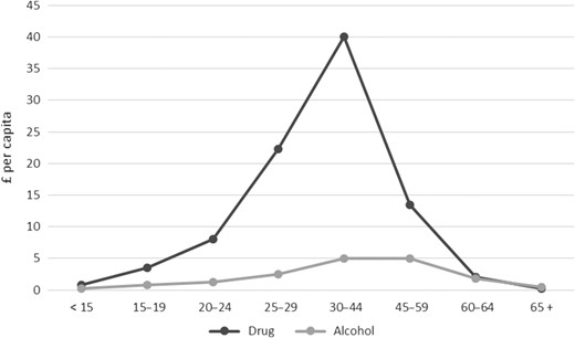
Mean annual costs per capita for drug and alcohol misuse treatment by age group (2013–14 data).
Predictors common to both the drugs misuse and the alcohol misuse model were SMR, IMD Crime, IMD Environment, population turnover, proportion male and proportion white British. A significant predictor in the drugs model but not the alcohol model was IMD Income. The final alcohol model contained the IMD mood and anxiety indicator; not a significant predictor in the drugs model. The final models achieved an adjusted R-squared of 0.513 for the drugs cost ratio but performed less well for the alcohol cost ratio (adjusted R-squared = 0.334).
Model 2: age-stratified model
Table 1 also shows the age-stratified model, applied separately to young people (under-18s) and adults (18+). The removal of the under-18s from the all-age group increased the adjusted R-squared statistic from 0.522 to 0.533. The model performed less well in the under-18s group (adjusted R-squared = 0.232). Variables which were significant predictors of the over-18s group were not significant in the under-18s (IMD Income, IMD Environment, proportion male, proportion GP prescribing and distance to nearest service). Mean waiting time was not significant in the over-18s but was in the under-18s. Additional potential predictor variables, such as proportion in full-time education, were explored to determine whether a better-performing model could be obtained for the under-18s but an adjusted R-squared of higher than 0.232 could not be achieved.
Within a drugs-only model a higher adjusted R-squared (0.526) was achieved for over-18s but was decreased (to 0.169) for under-18s. Within an alcohol-only model, a lower adjusted R-squared was achieved for both over-18s (0.327) and under-18s (0.160).
Model 3: person-based model
Table 2 presents the results of the person-based model for drug and alcohol misuse combined. The best-performing predictors in the model were: received prescribing in the past year; days treated in the past year; and whether treatment was completed in the previous year. These three variables together (plus age dummy variables) explained 46.9% of the variance in expenditure. The addition of other needs variables (SMR, population turnover and proportion male) and supply variables did not add substantially to the final adjusted R-squared statistic (0.470). When aggregated to area level for the purposes of comparison with other models, an R-squared statistic of 0.560 was achieved.
Person-based model, all ages, 2013/14 costs of drug and alcohol misuse treatment
| i | ii | iii | iv | |
|---|---|---|---|---|
| Age | ||||
| Age (15–19 years) | 3.09** | 1.06** | 0.96** | 0.99** |
| [0.167] | [0.101] | [0.108] | [0.113] | |
| Age (20–24) | 7.01** | 1.11** | 0.59** | 0.64** |
| [0.243] | [0.135] | [0.141] | [0.146] | |
| Age (25–29) | 22.31** | 4.30** | 3.95** | 4.04** |
| [0.421] | [0.187] | [0.191] | [0.197] | |
| Age (30–44) | 42.17** | 8.14** | 8.12** | 8.37** |
| [0.598] | [0.165] | [0.169] | [0.177] | |
| Age (45–59) | 16.81** | 2.36** | 2.55** | 2.64** |
| [0.287] | [0.114] | [0.119] | [0.125] | |
| Age (60–64) | 2.93** | −0.21* | 0.09 | 0.11 |
| [0.177] | [0.103] | [0.108] | [0.114] | |
| Age (65+) | −0.11 | −0.65** | −0.33** | −0.34** |
| [0.149] | [0.077] | [0.083] | [0.088] | |
| Individual treatment history | ||||
| Days of treatment previous year | 10.31** | 10.31** | 10.32** | |
| [0.042] | [0.042] | [0.042] | ||
| Completed treatment previous year | −1640.84** | −1641.03** | −1644.97** | |
| [6.475] | [6.474] | [6.527] | ||
| Received prescribing previous year | 1316.24** | 1315.91** | 1319.25** | |
| [13.569] | [13.569] | [13.658] | ||
| Area characteristics | ||||
| SMRa | 0.05** | 0.05** | ||
| [0.003] | [0.003] | |||
| Population turnover b | 0.03** | 0.03** | ||
| [0.002] | [0.003] | |||
| Proportion male | 25.92** | 30.05** | ||
| [3.856] | [4.257] | |||
| Supply variables | ||||
| Proportion of GP prescribing | −8.55** | |||
| [0.351] | ||||
| Distance to nearest servicec | −0.06** | |||
| [0.012] | ||||
| Mean waiting time | −0.01 | |||
| [0.009] | ||||
| Adjusted R-squared | 0.025 | 0.469 | 0.469 | 0.470 |
Notes: *P < 0.05. **P < 0.01. Reference category is age group 1 (under 15). aStandardized Mortality Ratio. bOutflow rate all ages: rate per 1000 (2009–10). cDistance (km) from post sector centroid to post code of the nearest treatment service. The dependent variable is drug and alcohol misuse expenditure for 2013/14. Unit of observation is the individual (n = 53 085 707). Robust standard errors in [ ]. All models account for UTLA.
Separate person-based models for drug and alcohol misuse services were considered. As with the combined model, the three best explanatory variables in both the drugs misuse and the alcohol misuse models were: received prescribing in the past year; days treated in the past year; and whether treatment was completed in the previous year. An adjusted R-squared of 0.490 was obtained in the drug misuse model and a much lower statistic (0.021) in the alcohol misuse model.
Impact of adoption of revised formula on target share
Figure 2 summarizes the impact that adoption of the revised person-based formula for substance misuse would have on existing target share. This shows the size of the impact plotted against a measure of overall deprivation (IMD 2010) and the proportion of young adults (18–30 year olds) for each LA. Adoption of the revised formula would have a net effect of redistributing more resources towards more deprived areas (higher IMD 2010 score). There is no corresponding shift in resources toward areas with a higher or lower proportion of young people.27
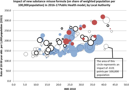
The impact of changing the substance misuse formula on LA target shares. Notes: solid circles indicate an increased target share, open circles a reduced target share, with the area of the circle proportional to the impact (London in solid red or dark shading/ bold, other in solid blue or light shading/ faint). Figure reproduced with permission from: Advisory Committee on Resource Allocation (ACRA) and the Department of Health, London (2015) Public health grant: proposed target allocation formula for 2016/17, https://www.gov.uk/government/consultations/public-health-formula-for-local-authorities-from-april-2016.
Discussion
We developed age-standardized, age-stratified and person-based models of substance misuse treatment costs by Local Authority in England, incorporating both need and supply variables to predict area-level variation in the costs of service provision. These were designed to better inform the allocation of substance misuse-specific public health budgets.
Main findings of this study
The age-standardized model performed well in predicting variation in the ratio of expected to actual cost by area (R-squared = 0.522). A separate model for alcohol misuse performed less well than that for drug misuse. The age-stratified model performed well for over-18s (R-squared = 0.533) but poorly for under-18s (R-squared = 0.232). The person-based model permits the use of a wider range of predictor variables, in particular, very strong predictors based on past-year treatment history. Predictive power was high for a model based on individual-level data (R-squared = 0.470) and conversion to area-level data for comparison purposes identified this model as the strongest of the three. For these reasons, we prefer the use of a person-based model of drug and alcohol misuse services.
What is already known on this topic
Resource allocation formulae have been used in healthcare in England since the 1970s. Needs estimates were generally amalgamated into a needs index, used to generate weighted populations to inform budget share. Developments introduced regional-level indicators to control for differences in supply (access) and non-need variables to control for differentially met need.10 Subsequent refinements incorporated age-stratification. More recently, person-based models have been developed where individual-level data are available. The existing substance misuse allocation formula3 is based on actual activity, need (SMR < 75) and performance. However, SMR is a narrow measure of need, supply-side and unmet-need biases were not accounted for and analyses were conducted at an aggregate level.
What this study adds
We aimed to develop a needs-based formula for distributing resources for substance misuse services that: expands the measures of need over that used currently; accounts for supply-side influences on the use of services; and estimates relative need using individual-level data.
We expanded on current measures of previous year service use data (incorporating days treated, treatment completion, receipt of prescription) and these were found to be strong predictors of current service use. Expanded measures of need, including population turnover and proportion male were also significant predictors of cost. The R-squared statistic achieved by our person-based model (0.470) was higher than that seen in similar work (0.123) to develop formulae to allocate resources for hospital care.12
Our analysis has shown that it is possible to generate statistical models that predict the costs of substance misuse services using measures of population need and supply characteristics. This included approaches to reduce confounding due to observed supply-side provision differences. A range of needs measures were consistently found to predict service use: SMR, the proportion of males in an area, age and population turnover. The ability to identify previous service use substantially improves explanatory power.
These models can be used to generate budgets that reflect variations in need across areas and therefore direct limited resources where they are needed most. Internationally, public health policies have the central aim of tackling inequalities in health.5 Socioeconomic factors, such as income and education, together with physical and social environmental factors, such as crime, are the main determinants of health inequalities.5 Of note, three IMD domains of deprivation, Income (models 1 and 2), Environment (models 1 and 2) and Crime (model 1) were important predictors of the ratio of actual to expected cost in our models, demonstrating the pivotal role of deprivation in describing the need for drug and alcohol misuse services. Adoption of our revised person-based formula for substance misuse would shift resources toward more deprived areas, thereby tackling health inequalities. At the time of writing, these models had not been adopted by the English Department of Health.
Limitations of this study
The available geographic level of analysis (postcode sector/LA combination) did not directly match that of available socio-demographic data, requiring the use of weighted population estimates.
Separate tariffs for alcohol or young people’s services were not available; costs were estimated based on adult drug service estimates. Explanatory power was lower for alcohol and young people’s models. There may be other predictors of these services that are not routinely collected. Although the alcohol model was not as strong, the best alcohol misuse model was highly correlated with the drug misuse model (r = 0.994); a combined model for drug and alcohol misuse was therefore recommended.
Whilst we were able to model observed confounding, there remains the possibility of unobserved confounding due to excluded supply-side factors that are correlated with our needs variables. There may also be measures of need that we have failed to source but that are valid and strong predictors of service use.
There are limitations of the existing approaches. First, the age-standardized approach may lead to biased age estimates—should these be correlated with the additional needs measures they could over- or under-represent the effects of age. In addition, such models impose a restriction that the additional needs measures have the same proportionate effect for all age groups. Age stratified models alleviate this issue to an extent, enabling additional needs measures and their estimated effects to vary across age groups. The recent transition towards a person-based approach enabled historic risk information for each individual captured in prior diagnoses to be factored into the formula. There is a concern that this information may contain non-need influences, such as supply factors that influence the probability of diagnosis. As a consequence, it is recommended to include a rich set of supply variables and include risk markers that are as independent as possible from unmeasured supply factors.28
In common with previous approaches to estimating resource allocation formulae for healthcare services in England, we have analysed variations in cost-weighted utilization and assumed that, once the effects of supply variables have been controlled for, the effects of population characteristics reflect differences in need. If there is systematic unmet need for some population groups, or differences in quality and effectiveness across population groups, this assumption is not met. The adoption of utilization to measure equity has been disputed for many years,29,30 but remains the preferred practical compromise in the absence of less imperfect, comprehensive measures of the need for resources.31
Acknowledgements
We are grateful to members of the UK Department of Health (DH) Technical Advisory Group (TAG) and the DH Advisory Committee on Resource Allocation (ACRA) for advice and comments and specifically would like to thank Michael Chaplin, Stephen Lorrimer and Keith Derbyshire from the Department of Health and Virginia Musto of Public Health England for their guidance and advice.
Conflicts of interest
None.
Funding
This work was supported by the UK Department of Health (DH) Policy Research Programme (now NIHR Policy Research Programme: grant number 085/0010). The views expressed are the sole responsibility of the authors and do not necessarily represent those of the UK DH Technical Advisory Group (TAG), the DH Advisory Committee on Resource Allocation (ACRA) or the Department of Health.
Disclaimer
This report relates to independent research commissioned and funded by the Department of Health Policy Research Programme.The views expressed in this publication are those of the author(s) and not necessarily those of the Department of Health, ‘arms’ length bodies and other government departments.
