Fast Stable Restricted Maximum Likelihood and Marginal Likelihood Estimation of Semiparametric Generalized Linear Models

Wood, Simon N.

doi:10.1111/j.1467-9868.2010.00749.x

Summary

Recent work by Reiss and Ogden provides a theoretical basis for sometimes preferring restricted maximum likelihood (REML) to generalized cross-validation (GCV) for smoothing parameter selection in semiparametric regression. However, existing REML or marginal likelihood (ML) based methods for semiparametric generalized linear models (GLMs) use iterative REML or ML estimation of the smoothing parameters of working linear approximations to the GLM. Such indirect schemes need not converge and fail to do so in a non-negligible proportion of practical analyses. By contrast, very reliable prediction error criteria smoothing parameter selection methods are available, based on direct optimization of GCV, or related criteria, for the GLM itself. Since such methods directly optimize properly defined functions of the smoothing parameters, they have much more reliable convergence properties. The paper develops the first such method for REML or ML estimation of smoothing parameters. A Laplace approximation is used to obtain an approximate REML or ML for any GLM, which is suitable for efficient direct optimization. This REML or ML criterion requires that Newton–Raphson iteration, rather than Fisher scoring, be used for GLM fitting, and a computationally stable approach to this is proposed. The REML or ML criterion itself is optimized by a Newton method, with the derivatives required obtained by a mixture of implicit differentiation and direct methods. The method will cope with numerical rank deficiency in the fitted model and in fact provides a slight improvement in numerical robustness on the earlier method of Wood for prediction error criteria based smoothness selection. Simulation results suggest that the new REML and ML methods offer some improvement in mean-square error performance relative to GCV or Akaike’s information criterion in most cases, without the small number of severe undersmoothing failures to which Akaike’s information criterion and GCV are prone. This is achieved at the same computational cost as GCV or Akaike’s information criterion. The new approach also eliminates the convergence failures of previous REML- or ML-based approaches for penalized GLMs and usually has lower computational cost than these alternatives. Example applications are presented in adaptive smoothing, scalar on function regression and generalized additive model selection.

Adaptive smoothing, Generalized additive mixed model, Generalized additive model, Generalized cross-validation, Marginal likelihood, Model selection, Penalized generalized linear model, Penalized regression splines, Restricted maximum likelihood, Scalar on function regression, Stable computation

1. Introduction

This paper is about reliable and efficient computation of likelihood-based smoothing parameter estimates in penalized generalized linear models (GLMs). Consider a GLM in which n independent univariate response variables y_i, with mean μ_i, depend on predictors via the model

g (μ_{i}) = X_{i}^{*} β^{*} + \sum_{j} L_{i j} f_{j}, y_{i} ~ an exponential family distribution,

(1)

where g is a known monotonic link function, the f_j are smooth but unknown functions of any number of covariates, the L_ij are known linear functionals (usually dependent on covariates) and

X_{i}^{*}

is the ith row of the model matrix for any strictly parametric model components, with corresponding coefficients β^*. Restriction to the exponential family implies that var(y_i) = φ V(μ_i), for some known ‘variance function’V and known or unknown ‘scale parameter’φ. Typical L_ijf_j- terms are f_j(x_i), f_j(x_i)z_i or ∫f_j(x) k_i(x) dx (where k_i is known), corresponding to generalized additive, varying coefficient and signal regression models respectively. For more on such models see, for example, Hastie and Tibshirani (1986, 1990), Ruppert et al. (2003), Wood (2006), Hastie and Tibshirani (1993), Marx and Eilers (1999), Ramsay and Silverman (2005), Reiss and Ogden (2007), Wahba (1990), Eilers and Marx (2002) and Fahrmeir et al. (2004).

To estimate model (1) in practice, the f_j can be represented by intermediate rank spline-type basis expansions (as originally proposed by Wahba (1980) and Parker and Rice (1985), for example), in which case the model becomes the GLM (Nelder and Wedderburn, 1972)

g (μ_{i}) = X_{i} β, y_{i} ~ an exponential family distribution,

(2)

where β now includes β^* and all the basis coefficients, and X is the corresponding n×q model matrix, with q usually substantially less than n. If the spline bases dimensions are sufficiently large to ensure reasonably low bias, then maximum likelihood estimation of model (2) will almost certainly lead to overfitting. To avoid this, the model should be estimated by penalized likelihood maximization, where the penalties suppress overly wiggly components f_j. In particular, the model is estimated by minimizing

D (β) + \sum_{j} λ_{j} β^{T} S_{j} β

(3)

with respect to β, where D is the model deviance, defined as the saturated log-likelihood minus the log-likelihood, all multiplied by 2φ (D is a useful GLM analogue of the residual sum of squares of a linear model, and working in terms of D will allow the direct use of some results from Wood (2008)); the S_j are q×q positive semidefinite matrices and the λ_j are positive smoothing parameters. Usually the β^TS_jβ measure the wiggliness of the f_j. In fact there may be several such penalties per f_j, e.g. when using tensor product (e.g. Wood (2006)) or adaptive (e.g. Krivobokova et al. (2008)) smoothing bases. The S_j may also be components of more general random-effects precision matrices.

Given the λ_j, there is a unique minimizer of expression (3), ${\hat{β}}_{λ}$ ⁠, which is straightforward to compute by a penalized version of the iteratively reweighted least squares method that is used for GLM estimation (penalized iteratively reweighted least squares (PIRLS)) (see for example Wood (2006) or Section 3.2). To select values for the λ_j requires optimization of a separate criterion, $V (λ)$ ⁠, say, which must be chosen.

1.1. Smoothness selection: prediction error or likelihood?

The λ_i selection criteria that have been proposed fall into two main classes. The first group try to minimize model prediction error, by optimizing criteria such as Akaike’s information criterion (AIC), cross-validation or generalized cross-validation (GCV) (see for example Wahba and Wold (1975) and Craven and Wahba (1979)). The second group treat the smooth functions as random effects (Kimeldorf and Wahba, 1970), so that the λ_i are variance parameters which can be estim- ated by maximum (marginal) likelihood (ML) (Anderssen and Bloomfield, 1974), or restricted maximum likelihood (REML), which Wahba (1985) called ‘generalized maximum likelihood’.

Asymptotically prediction error methods give better prediction error performance than likelihood-based methods (e.g. Wahba (1985) and Kauermann (2005)) but also have slower convergence of smoothing parameters to their optimal values (Härdle et al., 1988). Reflecting this, published simulation studies (e.g. Wahba (1985), Gu (2002), Ruppert et al. (2003) and Kohn et al. (1991)) differ about the relative performance of the two classes, although there is agreement that prediction error criteria are prone to occasional severe undersmoothing. Reiss and Ogden (2009) provided a theoretical comparison of REML and GCV at finite sample sizes, showing that GCV is both more likely to develop multiple minima and to give more variable λ_j-estimates. Fig. 1 illustrates the basic issue. GCV penalizes overfit only weakly, with a minimum that tends to be very shallow on the undersmoothing side, relative to sampling variability. This can lead to an overfit. By contrast, REML (and also ML) penalizes overfit more severely and therefore tends to have a much more pronounced optimum, relative to sampling variability. In principle, extreme undersmoothing can also be avoided by use of modified prediction error criteria such as AICc (Hurvich et al., 1998), but in practice the use of low to intermediate rank bases for the f_j already suppresses severe overfit, and AICc then offers little additional benefit relative to GCV, as Fig. 1 also illustrates.

Fig. 1

Example comparison of GCV, AICc and REML criteria: (a) some (x,y)-data modelled as yi = f(xi)+ɛi, ɛi independent and identically distributed N(0,σ2) where smooth function f was represented by using a rank 20 thin plate regression spline (Wood, 2003); (b)–(d) various smoothness selection criteria plotted against logarithmic smoothing parameters, for 10 replicates of the data (each generated from the same ‘truth’) (note how shallow the GCV and AICc minima are relative to the sampling variability, resulting in rather variable optimal λ-values (which are shown as a rug plot), and a propensity to undersmooth; in contrast the REML optima are much better defined, relative to the sampling variability, resulting in a smaller range of λ-estimates); (e)–(h) are equivalent to (a)–(d), but for data with no signal, so that the appropriate smoothing parameter should tend to ∞ (note GCV’s and AICc’s occasional multiple minima and undersmoothing in this case, compared with the excellent behaviour of REML; ML (which is not shown) has a similar shape to REML)

Open in new tab Download slide

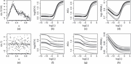
Example comparison of GCV, AICc and REML criteria: (a) some (x,y)-data modelled as y_i = f(x_i)+ɛ_i, ɛ_i independent and identically distributed N(0,σ²) where smooth function f was represented by using a rank 20 thin plate regression spline (Wood, 2003); (b)–(d) various smoothness selection criteria plotted against logarithmic smoothing parameters, for 10 replicates of the data (each generated from the same ‘truth’) (note how shallow the GCV and AICc minima are relative to the sampling variability, resulting in rather variable optimal λ-values (which are shown as a rug plot), and a propensity to undersmooth; in contrast the REML optima are much better defined, relative to the sampling variability, resulting in a smaller range of λ-estimates); (e)–(h) are equivalent to (a)–(d), but for data with no signal, so that the appropriate smoothing parameter should tend to ∞ (note GCV’s and AICc’s occasional multiple minima and undersmoothing in this case, compared with the excellent behaviour of REML; ML (which is not shown) has a similar shape to REML)

Greater resistance to overfit, less smoothing parameter variability and a reduced tendency to multiple minima suggest that REML or ML might be preferable to GCV for semiparametric GLM estimation. But these benefits must be weighed against the fact that existing computational methods for REML or ML estimation of semiparametric GLMs are substantially less reliable than their prediction error equivalents, as the remainder of this section explains.

There are two main classes of computational method for λ_j-estimation: those based on single iterations and those based on nested iterations. In the single-iteration case, each PIRLS step, which is used to update $\hat{β}$ ⁠, is supplemented by a $\hat{λ}$ -update. The latter is based on improving a λ selection criterion $V_{\hat{β}} (λ)$ ⁠, which depends on the estimate of $\hat{β}$ at the start of the step. $V_{\hat{β}} (λ)$ will be some sort of REML, GCV or similar criterion, but it is not a fixed function of λ, instead changing with $\hat{β}$ from iterate to iterate. Consequently single-iteration methods do not guarantee convergence to a fixed $\hat{λ}$ ⁠, ${\hat{β}}_{\hat{λ}}$ (see Gu (2002), page 154, Wood (2006), page 180, and Brezger et al. (2007), reference manual section 8.1.2).

In nested iteration, the smoothness selection criterion $V (λ)$ depends on β only via ${\hat{β}}_{λ}$ ⁠. An outer iteration updates $\hat{λ}$ to optimize $V (λ)$ ⁠, with each iterative step requiring an inner PIRLS iteration to find the current ${\hat{β}}_{λ}$ ⁠. Because nested iteration optimizes a properly defined function of λ, it is possible to guarantee convergence to a fixed optimum, provided that $V$ is bounded below, and expression (3) has a well-defined optimum (conditions which are rather mild, in practice). The disadvantage of nested iteration is substantially increased computational complexity.

To date only single-iteration methods have been proposed for REML or ML estimation of semiparametric GLMs (e.g. Wood (2004), using Breslow and Clayton (1993), or Fahrmeir et al. (2004), using Harville (1977)), and in practice convergence problems are not unusual: examples are provided in Wood (2004, 2008), and in Appendix A. Early prediction-error-based methods were also based on single iteration (e.g. Gu (1992) and Wood (2004)), and suffered similar convergence problems, but these were overcome by Wood’s (2008) nested iteration method for GCV, generalized approximate cross-validation, and AIC smoothness selection. Wood (2008) cannot be extended to REML or ML while maintaining good numerical stability, so the purpose of this paper is to provide an efficient and stable nested iteration method for REML or ML smoothness selection, thereby removing the major practical obstacle to use of these criteria.

2. Approximate restricted maximum likelihood or marginal likelihood for generalized linear model smoothing parameter estimation

Since the work of Kimeldorf and Wahba (1970), Wahba (1983) and Silverman (1985), it has been recognized that the penalized likelihood estimates $\hat{β}$ are also the posterior modes of the distribution of β|y, if β∼N(0,S⁻φ), where S=Σ_i λ_iS_i, and S⁻ is an appropriate generalized inverse (see for example Wood (2006)). Once the elements of β are viewed as random effects in this way, it is natural to try to estimate the λ_i, and possibly φ, by ML or REML (Wahba, 1985).

This preliminary section uses standard methods to obtain an approximate REML expression that is suitable for efficient direct optimization to estimate the smoothing parameters of a semiparametric GLM. Rather than follow Patterson and Thompson (1971) directly, Laird and Ware’s (1982) approach to REML is taken, in which fixed effects are viewed as random effects with improper uniform priors and are integrated out. The key feature of the resulting expression is that it is relatively efficient to compute with and is suitable for optimizing as a properly defined function of the smoothing parameters, i.e., in contrast with previous single-iteration approaches to this problem, there is no need to resort to optimizing the REML score of a working model. Since a very similar approach obtains an approximate ML, this is also derived. ML can be useful for comparing models with different smooth terms included, for example (REML cannot be used for such a comparison because the alternative models will differ in fixed effect structure).

Consider a penalized GLM with log-likelihood l(β)= log {f_y(y|β)}. Under the random-effects formulation we have an improper ‘prior’ density for β,

f_{β} (β) = \frac{| S / ϕ |_{+}^{0.5}}{\sqrt{{(2 π)}^{n_{b} - M_{p}}}} \exp (\frac{- β^{T} S β}{2 ϕ}),

where |B|₊ denotes the product of the non-zero eigenvalues of B. n_b is the dimension of β and M_p is the dimension of the null space of S. To obtain the restricted likelihood for REML we need to integrate β out of f(y,β) = f_y(y|β) f_β(β) (for ML we would need to integrate out the part of β that is in the range space of S). In practice the integral can be approximated as follows. Let H=−∂²l/∂β ∂β^T, and

\hat{β}

be the maximizer of f(y,β), i.e. the penalized likelihood estimates. Then

\begin{matrix} f (y, β) ≃ \exp [\log \{f_{y} (y ∣ \hat{β})\} + \log \{f_{β} (\hat{β})\} - {(β - \hat{β})}^{T} (H + S / ϕ) (β - \hat{β}) / 2] \\ = f_{y} (y ∣ \hat{β}) f_{β} (\hat{β}) \exp \{- {(β - \hat{β})}^{T} (H + S / ϕ) (β - \hat{β}) / 2\} . \end{matrix}

Integrating with respect to β, and denoting the likelihood by L, we obtain the Laplace approximate REML criterion

L_{R} (λ, ϕ) = L (\hat{β}) f_{β} (\hat{β}) \frac{\sqrt{{(2 π)}^{n_{b}}}}{| H + S / ϕ |^{0.5}}

(which is actually exact for Gaussian models with the identity link), i.e., defining l_r = log(L_r),

2 l_{r} = 2 l (\hat{β}) + \log (| S / ϕ |_{+}) - {\hat{β}}^{T} S \hat{β} / ϕ - \log | H + S / ϕ | + M_{p} \log (2 π) .

If the penalized GLM has its coefficients estimated by Newton-based PIRLS, as suggested below, then H = X^TWX/φ, where W is a diagonal weight matrix. To obtain ML, rather than REML, we would need to reparameterize to separate the parameters into penalized and unpenalized. Then H would be the negative Hessian for the penalized parameters only: further details are provided below in Section 2.1.

For ease of computation it helps to separate out l_r into φ-dependent and φ-independent components. For this, let l_s(φ) denote the saturated log-likelihood and define

D_{p} = D (\hat{β}) + {\hat{β}}^{T} S \hat{β}

and (assuming Newton weights)

K = \{\log |X^{T} W X + S| - \log (| S |_{+})\} / 2.

We then have that

- l_{r} = \frac{D_{p}}{2 ϕ} - l_{s} (ϕ) + K - \frac{M_{p}}{2} \log (2 π ϕ) .

(4)

There are two approaches to the estimation of φ:

(a)
estimate φ as part of l_r-maximization, or
(b)
use the Pearson statistic over n−M_p as $\hat{ϕ}$ ⁠, and optimize the resulting criterion, taking account of the derivatives of $\hat{ϕ}$ with respect to the smoothing parameters.

The only advantage of approach (b) is that it may sometimes allow the resulting REML score to be used as a heuristic method of smoothness selection with quasi-likelihood.

The simpler approach of using the expected Hessian in place of H was also investigated, but in simulations it gave worse performance than GCV when non-canonical links were used.

2.1. Marginal likelihood details

For Laplace approximate ML, rather than REML, estimation, the only difference to the criterion is that we now need H to be the negative Hessian with respect to the coefficients of any orthogonal basis for the range space of the penalty. The easiest way to separate out the range space is to form the eigendecomposition

\sum_{j} S_{j} / {‖S_{j}‖}_{F} = U Λ U^{T},

where the scaling of each S_j by its Frobenius norm maintains good numerical conditioning. The first q−M_p columns of U now form an orthogonal basis for the range space of S (see for example Wood (2006), sections 4.8.2 and 6.6.1). In consequence, if we reparameterize by setting

\bar{β} = U^{T} β

then the first q−M_p elements of

\bar{β}

will be penalized and should be integrated out of the joint density of y and

\bar{β}

⁠, whereas the last M_p elements are unpenalized, and hence left alone. Let U₁ be the first q−M_p columns of U. Applying the reparameterization we have

\bar{X} = X U_{1}

and

\bar{S} = U_{1}^{T} S U_{1}

⁠, and some work establishes that the negative (Laplace approximate) log-marginal-likelihood is

- l = \frac{D_{p}}{2 ϕ} - l_{s} (ϕ) + \frac{\log |{\bar{X}}^{T} W \bar{X} + \bar{S}| - \log (| S |_{+})}{2} .

(5)

2.2. Accuracy of the Laplace approximation

For fixed dimension of β, the true REML or ML integral divided by its Laplace approximation is 1+O(n⁻¹) (see for example Davison (2003), section 11.3.1). For consistency, it is usually necessary for the dimension of β to grow with n, which reduces this rate somewhat. However, for spline-type smoothers the dimension need only grow slowly with n (for example Gu and Kim (2002) showed that the rate need only be O(n^2/9) for cubic-spline-like smooths), so convergence is still rapid. Kauermann et al. (2009) showed in detail that the Laplace approximation is well justified asymptotically for ML in the penalized regression spline setting.

Rapid convergence does not in itself guarantee that the approximation is sufficiently accurate for any particular finite sample. Fortunately a simple and computationally efficient accuracy check is readily implemented, since a rather precise unbiased estimator of the REML score can be obtained by importance sampling with a ‘Laplace proposal’. In particular, if R is a square factor such that

R^{T} R = {(X^{T} W X + S)}^{- 1} \hat{ϕ},

and z_i are n_s independent N(0,I) random n_b vectors, then

\frac{{(2 π)}^{n_{b} / 2}}{n_{s} | R |} \sum_{i = 1}^{n_{s}} f_{y} (y ∣ \hat{β} + R^{T} z_{i}) f_{β} (\hat{β} + R^{T} z_{i}) \exp (\frac{{‖z_{i}‖}^{2}}{2})

is an unbiased estimator of the exact REML score (see, for example, Monahan (2001), section 10.4C). In the work that is reported here n_s in the range 1000–10000 was sufficient to ensure that the Monte Carlo variability was at least an order of magnitude smaller than the mean difference between the estimator and the deterministic Laplace approximation. This estimator was used to estimate the Laplace approximation error, at the estimated smoothing parameters, for all the examples that are presented subsequently in this paper. The worst error was for the binary simulations in Section 4, where the magnitude of the error was up to 0.3. The other examples had approximation errors that were an order of magnitude smaller. Hence the error that is induced by the deterministic Laplace approximation is not significant relative to the sampling uncertainty in the smoothing parameters, suggesting that the Laplace approximation is adequate for the examples that are presented here.

Note that the Laplace approximation that is employed here does not suffer from the difficulties that are common to most penalized quasi-likelihood (PQL) (Breslow and Clayton, 1993) implementations when used with binary data. Most PQL implementations must estimate φ for the working model, even with binary data where this is not really satisfactory. In addition, PQL uses the expected Hessian in place of the exact Hessian when non-canonical links are used, which also reduces accuracy. That said, it should still be expected that the accuracy of equations (4) and (5) will reduce for binary or Poisson data when the expectation of the response variable is very low.

3. Optimizing the restricted maximum likelihood criterion

Equations (4) and (5) depend on the smoothing parameter vector λ via the dependence of S and $\hat{β}$ (and hence W) on λ. The proposal here is to optimize equation (4) or (5) with respect to the ρ_i = log (λ_i), by using Newton’s method, with the usual modifications that

(a)
some step length control will be used and
(b)
the Hessian will be perturbed to be positive definite, if it is not (see Nocedal and Wright (2006) for an up-to-date treatment and computational details).

Each trial logarithmic smoothing parameter vector ρ, proposed as part of the Newton method iteration, will require a PIRLS iteration to evaluate the corresponding $\hat{β}$ (and hence W). So the whole optimization consists of two nested iterations: an outer iteration to find $\hat{ρ}$ ⁠, and an inner iteration to find the $\hat{β}$ corresponding to any ρ. The outer iteration requires the gradient and Hessian of equation (4) or (5) with respect to ρ, and this in turn requires first and second derivatives of $\hat{β}$ with respect to ρ.

Irrespective of the details of the optimization method, the major difficulty in minimizing equation (4) or (5) is that, if some λ_j is sufficiently large, then the ‘numerical footprint’ of the corresponding penalty term λ_jβ^TS_jβ can extend well beyond the penalty’s range space, i.e. numerically the penalty can have marked effects in the subspace of the model parameter space for which, formally, β^TS_jβ=0. For example if ‖λ_jS_j‖≫‖λ_kS_k‖ then λ_jS_j can have effects which are ‘numerically zero’ when judged relatively to ‖λ_jS_j‖ (and would be exactly zero in infinite precision arithmetic), but which are larger than the strictly non-zero effects of λ_kS_k. If left uncorrected, this problem leads to serious errors in evaluation of $\hat{β}$ ⁠, |S|₊ and |X^TWX+S| and their derivatives with respect to ρ (see Section 3.1). Because multiple penalties often have overlapping range spaces (i.e. they penalize intersecting subspaces of the parameter space), no single reparameterization can solve this problem for all λ-values, but an adaptive reparameterization approach does work and is outlined in Section 3.1. Note that the Wood (2008) method, for dealing with numerical ill conditioning for prediction error criteria, is hopeless here. That method truncates the parameter space to deal with ill conditioning that is induced by changes in λ, but such an approach would lead to large erroneous and discontinuous changes in |S|₊ and |X^TWX+S| as λ changes. We shall of course still need to truncate the parameter space if some parameters would not be identifiable whatever the value of λ, but such a λ-independent truncation is not problematic.

A second question, when minimizing equation (4) or (5), is what optimization method to use to obtain the ${\hat{β}}_{λ}$ corresponding to any trial λ. If a PIRLS scheme is employed based on Newton (rather than Fisher) updates, then the Hessian that is required in equation (4) or (5) is conveniently obtained as a by-product of fitting, which also means that the same method can be used to stabilize both $\hat{β}$ and REML or ML evaluation. Furthermore the required derivatives of $\hat{β}$ with respect to ρ can be obtained directly from the information that is available as part of the PIRLS, using implicit differentiation, without the need for further iteration. Newton-based PIRLS also leads to more rapid convergence with non-canonical links.

As a result of the preceding considerations, this paper proposes that the following steps should be taken for each trial ρ proposed by the outer Newton iteration.

Step 1: reparameterize to avoid large norm λ_jS_j-terms having effects outside their range spaces, thereby ensuring accurate computation with the current ρ (Section 3.1).
Step 2: estimate $\hat{β}$ by Newton-based PIRLS, setting to 0 any elements of $\hat{β}$ which would be unidentifiable irrespectively of the value ofρ (Sections 3.2 and 3.3).
Step 3: obtain first and second derivatives of $\hat{β}$ with respect to ρ, using implicit differentiation and the quantities that are calculated as part of step 2 (Section 3.4).
Step 4: using the results from steps 2 and 3, evaluate the REML or ML criterion and derivatives with respect to ρ (Section 3.5).

After these four steps, all the ingredients are in place to propose a new ρ by using a further step of Newton’s method.

3.1. Reparameterization, log|S|₊ and √S

log (|S|₊) (where S=Σ_j λ_jS_j) is the most numerically troublesome term in the REML or ML objective. Both λ_i→0 and λ_i→∞ can cause numerical problems when evaluating the determinant. The problem is most easily seen by considering the simple example of evaluating |λ₁S₁+λ₂S₂| when the q×q positive semidefinite dense matrices S_j are not full rank, but λ₁S₁+λ₂S₂ is. In what follows let ‖·‖ denote the matrix 2-norm (although the 1-, ∞- or Frobenius norms would serve as well), and let $\hat{x}$ denote the computed version of any quantity x. Consider a similarity transform based on the eigendecomposition S₁ = UΛU^T, with computed version $S_{1} = \hat{U} \hat{Λ} {\hat{U}}^{T}$ ⁠. Let Λ⁺ denote the vector of strictly positive eigenvalues, and Λ⁰ the vector of zero eigenvalues, and note that ${\hat{Λ}}^{0}$ will have elements of typical magnitude ‖S₁‖ɛ_m where ɛ_m is the computational machine precision (see for example Watkins (1991), section 5.5, or Golub and van Loan (1996), chapter 8).

By standard properties of similarity transforms we have

|λ_{1} S_{1} + λ_{2} S_{2}| = |λ_{1} Λ + λ_{2} U^{T} S_{2} U| .

(6)

Suppose that S_j has rank r_j and rank deficiency d_j = q−r_j. As λ₁/λ₂→∞ it is routine that the r₁ largest eigenvalues of λ₁S₁+λ₂S₂→λ₁Λ⁺, so

|λ_{1} S_{1} + λ_{2} S_{2}| \to λ_{1}^{r_{1}} \prod_{i} Λ_{i}^{+} α,

where the factor α depends on λ₂S₂. However, as λ₁/λ₂→∞all the computed eigenvalues of

λ_{1} S_{1} + λ_{2} S_{2} \to λ_{1} \hat{Λ}

⁠, so

|λ_{1} \hat{S_{1} + λ_{2}} S_{2}| \to λ_{1}^{r_{1}} \prod_{i} {\hat{Λ}}_{i}^{+} λ_{1}^{d_{1}} \prod_{i} {\hat{Λ}}_{i}^{0} .

Hence the computed determinant is seriously in error because the factor

λ_{1}^{d_{1}} Π_{i} {\hat{Λ}}_{i}^{0}

is essentially arbitrary and is unrelated to the correct factor α. (Note that the problem vanishes for a full rank S₁.)

The difficulty arises because the computed version of the matrix λ₁Λ+λ₂U^TS₂U is perturbed by the completely arbitrary error terms in

λ_{1} {\hat{Λ}}^{0}

⁠. In general the effect of a perturbation on the determinant of a positive definite A, with eigenvalues Λ^A, depends on the size of the perturbation relative to min(Λ^A). This is easily seen by considering a simple additive perturbation ɛI (where ɛ is the size of perturbation). Then

| A + ε I | / | A | = \prod_{i} (Λ_{i}^{A} + ε) / Λ_{i}^{A},

where the largest contribution to the right-hand side is from the term {min(Λ^A)+ɛ}/min(Λ^A). Hence we can expect problems when the perturbations

λ_{1} {\hat{Λ}}^{0}

become non-negligible relative to the smallest eigenvalue of λ₁S₁+λ₂S₂, which is bounded below by the smallest positive eigenvalue of λ₂S₂ as λ₁/λ₂→∞.

In short, we can expect this ‘numerical zero leakage’ issue to spoil determinant calculations whenever the ratio of the largest strictly positive eigenvalue of λ₁S₁ (which sets the scale of the arbitrary perturbation, $λ_{1} {\hat{Λ}}^{0}$ ⁠) to the smallest strictly positive eigenvalue of λ₂S₂ is too great. However, the example also suggests a simple way of suppressing the problem. Reparameterize by using the computed eigenbasis of the dominant term S₁, so that S₁ becomes $\hat{Λ}$ and S₂ becomes ${\hat{U}}^{T} S_{2} \hat{U}$ ⁠. In the transformed space it is easy to ensure that the dominant term (now $\hat{Λ}$ ⁠) acts only within its range space, by setting ${\hat{Λ}}^{0} = 0$ (if the rank of S₁ is known then identifying which eigenvalues should be 0 is trivial; if not, see step 3 in Appendix B).

Having reparameterized and truncated in this way, stable evaluation of |λ₁Λ+λ₂U^TS₂U| is straightforward. Only the first r₁ columns of $λ_{1} \hat{Λ} + λ_{2} {\hat{U}}^{T} S_{2} \hat{U}$ now depend on λ₁S₁. Forming a pivoted QR-decomposition $λ_{1} \hat{Λ} + λ_{2} {\hat{U}}^{T} S_{2} \hat{U} = \hat{Q} \hat{R}$ maintains this column separation in $\hat{R}$ (the decomposition acts on columns, without mixing between columns), with the result that $|λ_{1} \hat{S_{1} + λ_{2}} S_{2}| = |λ_{1} \hat{Λ} + λ_{2} {\hat{U}}^{T} S_{2} \hat{U}| = Π_{i} {\hat{R}}_{i i}$ can be accurately computed. Furthermore, pivoting ensures that ${\hat{R}}^{- 1}$ is computable, which is necessary for derivative calculations. See Golub and van Loan (1996) for full discussion of QR-decomposition with pivoting.

The stable computation of $\hat{β}$ ⁠, which was discussed in Section 3.3, will also require that a square root of S can be formed that maintains the required ‘column separation’ of the dominant terms in S (i.e. we must not end up with large magnitude elements in some column j>r₁, just because λ₁‖S₁‖ is large). This is quite straightforward under the reparameterization that was just discussed. For example, let ${\hat{S}}^{'} = λ_{1} \hat{Λ} + λ_{2} {\hat{U}}^{T} S_{2} \hat{U}$ (with $\hat{Λ}$ s ‘machine zeros’ set to true zeros) and $\hat{P}$ be the diagonal matrix such that ${\hat{P}}_{i i} = \sqrt{|{\hat{S}}_{i i}^{'}|}$ ⁠. Forming the Choleski decomposition $\hat{L} {\hat{L}}^{T} = {\hat{P}}^{- 1} {\hat{S}}^{'} {\hat{P}}^{- 1}$ ⁠, then $\hat{E} = {\hat{L}}^{T} \hat{P}$ is a matrix square root such that $\hat{E} \hat{T} E = {\hat{S}}^{'}$ ⁠. Furthermore, λ₁S₁ affects only the size of the elements in $\hat{E}$ ’s first r₁ columns (this is easily seen, since, from the definition of $\hat{E}$ ⁠, the squared Euclidean norm of its jth column is given by ${\hat{S}}_{j j}^{'}$ ⁠, which does not depend on λ₁S₁ if j>r₁). The preconditioning (or ‘scaling’) matrix ${\hat{P}}^{- 1}$ ensures that the Choleski factor can be computed in finite precision, however divergent the sizes of the components of S (see for example Watkins (1991), section 2.9). From now on no further purpose is served by distinguishing between ‘true’ and computed quantities, so circumflexes will be omitted.

Of course S=Σ λ_iS_i generally contains more than two terms and is not full rank, but Appendix B generalizes the similarity-transform-based reparameterization, along with the (generalized) determinant and square-root calculations, to any number of components of a rank deficient S. It also provides the expressions for the derivatives of log (|S|₊) with respect to ρ. The operations count for Appendix B is O(q³).

The stable matrix square root E, produced by the Appendix B method, is only useful if the rest of the model fitting adopts the Appendix B reparameterization, i.e. the transformed S_i, S and E, computed by Appendix B, must be used in place of the original untransformed versions, along with a transformed version of the model matrix. To compute the latter, let Q_s be the orthogonal matrix describing the similarity transform applied by Appendix B, i.e., if S is the transformed total penalty matrix, then formally $Q_{s} S Q_{s}^{T}$ is the untransformed original. Then the transformed model matrix should be XQ_s (obtained at O(nq²) cost). In what follows it is assumed that this reparameterization is always adopted, being recomputed for each new ρ-value. So the model matrix and penalty matrices are taken to be the transformed versions, from now on. If the coefficient estimates in this parameterization are $\hat{β}$ ⁠, then the estimates in the original parameterization are $Q_{s} \hat{β}$ ⁠.

Finally, reparameterization is preferable to simply limiting the working λ-range. To keep the non-zero eigenvalues of all λ_iS_i within limits that guarantee computational stability usually entails unacceptably restrictive limits on the λ_i, i.e. limits that are sufficiently restrictive to ensure numerical stability have statistically noticeable effects.

3.2. Estimating the regression coefficients given smoothing parameters

Minimizing expression (3) by Newton’s method or Fisher scoring both result in a PIRLS method, as follows. Pseudodata and weights are defined first:

\begin{matrix} z_{i} = η_{i} + \frac{(y_{i} - μ_{i}) g_{i}^{'}}{α_{i}}, \\ w_{i} = \frac{ω_{i} α_{i}}{V_{i} g_{i}^{' 2}}, \end{matrix}

where η_i = g(μ_i) = X_iβ,V_i = V(μ_i),

α_{i} = \{\begin{array}{l} 1 + (y_{i} - μ_{i}) (V_{i}^{'} / V_{i} + g_{i}^{''} / g_{i}^{'}) & for Newton' s method, \\ 1 & for Fisher scoring \end{array}

and x^′ denotes dx/dμ_i, whatever x. These quantities are always evaluated at the current μ_i-estimates. The ω_i are any prior weights and are usually 1. If a canonical link function is used then α_i = 1,∀i, and Newton’s method and Fisher scoring coincide.

Estimation of the coefficients β is performed by the modified IRLS scheme of iterating the following two steps to convergence (μ-estimates are initialized by using the previous ${\hat{β}}_{λ}$ ⁠, or directly from y).

Step 1: given the current estimate of μ (and hence η), evaluate z and w.
Step 2: solve the weighted penalized least squares problem of minimizing
$\sum_{i = 1}^{n} w_{i} {(z_{i} - X_{i} β)}^{2} + \sum_{j} λ_{j} β^{T} S_{j} β$
(7)
with respect to β, to obtain the updated estimate of β and hence μ (and η). See Section 3.3.

At convergence of the Newton-type iteration the Hessian of the deviance with respect to β is given by 2X^TWX, where W=diag(w_i). Under Fisher scoring 2X^TWX is the expected Hessian. See for example Green and Silverman (1994) or Wood (2006) for further information on (Fisher-based) PIRLS.

Several points should be noted.

(a)
Step halving will be needed in the event that the penalized deviance increases at any iteration, but the Newton method should never require it at the end of the iteration.
(b)
The Newton scheme tends to converge faster than Fisher scoring in non-canonical link situations, an effect which can be particularly marked when using Tweedie (1984) distributions.
(c)
With non-canonical links, the w_i need not all be positive for the Newton scheme, and in practice negative weights are encountered for perfectly reasonable models: the next section deals with this. Negative w_i provide the second reason that the Wood (2008) method cannot be extended to REML.

3.3. Stable least squares with negative weights

This section develops a method for stable computation of weighted least squares problems when some weights are negative, as required by the Newton-based PIRLS that was described in Section 3.2. The method also deals with identifiability problems that do not depend on the magnitude of λ.

The obvious approach to solving expression (7) in the presence of negative weights would be to solve directly

(X^{T} W X + S) \hat{β} = X^{T} W z

(8)

for

\hat{β}

⁠, where W=diag(w_i), z is the vector of z_i from Section 3.2 and S=Σ_jλ_jS_j. However, it is well known that direct formation of X^TWX results in a system with a condition number that is the square of what is necessary (see for example Golub and van Loan (1996), sections 5.3.2 and 5.3.8). Given that penalized GLMs are frequently complex models in which concurvity effects can easily lead to quite high condition numbers, this approach is not sensible.

When weights are non-negative, a stable solution of equation (8) is based on orthogonal decomposition of √WX (e.g. Wood (2004)), but this does not work if some weights are negative. This section proposes a stable solution method, by starting with a ‘nearby’ penalized least squares problem, for which all the weights are non-negative, applying a stable orthogonal decomposition approach to this, but at the same time developing the correction terms that are necessary to end up with the solution to equation (8) itself.

To make progress then, let W⁻ denote the diagonal matrix such that

W_{i i}^{-}

equals 0 if w_i⩾0 and −w_i otherwise. Also let

\bar{W}

be a diagonal matrix with

{\bar{W}}_{i i} = |w_{i}|

⁠. In this case

X^{T} W X = X^{T} \bar{W} X - 2 X^{T} W^{-} X .

So X^TWX has been split into a component that is straightforward to compute with stably, and a ‘correction’ term. Starting with the straightforward term, perform a QR-decomposition

\sqrt{W} X = Q R

(9)

(either without pivoting, or reversing the pivoting of

R

after the decomposition). At this stage it is necessary to test for any inherent lack of identifiability in the problem (i.e. lack of identifiability which is λ independent). Section 3.3.1 describes how to do this. For the moment suppose that the inherent rank of the problem is r, and we have a list of any unidentifiable parameters. Then drop the columns of

R

and X and the rows and columns of the S_i corresponding to any unidentifiable parameters.

R

is now a square root of

X^{T} \bar{W} X

⁠, but we really need a square root of

X^{T} \bar{W} X + S

⁠, to move towards solution of equation (8). For this, let E be a matrix such that E^TE = S, computed as described in Appendix B and Section 3.1. Drop the columns of E corresponding to any unidentifiable parameters, and form a further pivoted QR-decomposition

(\begin{array}{l} R \\ E \end{array}) = Q R .

(10)

R is the required pivoted square root of

X^{T} \bar{W} X + S

⁠. Now define n×r matrix

Q_{1} = Q Q [1 : q,]

⁠, where q is the number of columns of X and Q[1:q,] denotes the first q rows of Q. Hence

\sqrt{W} X = Q_{1} R .

(11)

For what follows, the pivoting that is used in the QR-step (10) will have to be applied to the rows and columns of S_j and the columns of X.

Now we need to correct the matrix square root R to obtain what is actually needed to solve equation (8):

\begin{matrix} X^{T} W X + S = R^{T} R - 2 X^{T} W^{-} X \\ = R^{T} (I - 2 R^{- T} X^{T} W^{-} X R^{- 1}) R \\ = R^{T} (I - 2 R^{- T} R^{T} Q_{1}^{T} I^{-} Q_{1} R R^{- 1}) R \\ = R^{T} (I - 2 Q_{1}^{T} I^{-} Q_{1}) R, \end{matrix}

where I⁻ denotes the diagonal matrix such that

I_{i i}^{-}

equals 0 if w_i>0 and 1 otherwise, and

W^{-} = I^{-} \bar{W}

⁠. The matrix

I - 2 Q_{1}^{T} I^{-} Q_{1}

is not necessarily positive semidefinite and so requires careful handling. Forming the singular value decomposition

I^{-} Q_{1} = U D V^{T}

(12)

(of course, in practice the zero rows of I⁻Q₁ can be dropped before decomposition) then we obtain

\begin{matrix} X^{T} W X + S = R^{T} (I - 2 V D^{2} V^{T}) R \\ = R^{T} V (I - 2 D^{2}) V^{T} R \end{matrix}

(13)

(and additionally

X^{T} W X = R^{T} R - 2 R^{T} V D^{2} V^{T} R)

⁠). Now define

\begin{array}{l} P = R^{- 1} V {(I - 2 D^{2})}^{- 1 / 2}, \\ K = Q_{1} V {(I - 2 D^{2})}^{- 1 / 2} . \end{array}

(14)

If

\bar{z}

is the vector such that

{\bar{z}}_{i} = z_{i}

if w_i⩾0 and

{\bar{z}}_{i} = - z_{i}

otherwise, then substituting from equations (14), (13) and (11) into (8) and solving gives

\hat{β} = P K^{T} \sqrt{W} \bar{z} .

The key point about this calculation is that its condition number will be dominated by that of R, the matrix which must be inverted in the definition of P. This is approximately the square root of the condition number for using X^TWX+S directly, since the term to be inverted in this latter case would be dominated by R^TR (see Golub and van Loan (1996), sections 2.7.2 and 3.5.4 if this is unclear). The key computational steps that are involved in finding

\hat{β}

are equations (9), (10), (12) and (14), plus the rank identification of Section 3.3.1.

Given equation (13), it is now possible to compute one of the REML log-determinant components by using

|X^{T} W X + S| = | R |^{2} |I - 2 D^{2}|,

and it is also worth noting, from equations (13) and (14), that (X^TWX+S)⁻¹ = PP^T (strictly some sort of pseudoinverse if there is rank deficiency).

There is an important additional detail. At the penalized MLE, X^TWX+S will be positive semidefinite, so d_i⩽1/√2 (reparameterize so that R is the identity to see this), but en route to the optimum there is no guarantee that the penalized likelihood is positive semidefinite. So, if d_i>1/√2, for any i, then a Fisher step should be substituted, i.e. set α_i = 1, so that w_i⩾0, ∀i. Then

P = R^{- 1} and K = Q_{1}

and the expression for

\hat{β}

⁠, above, simplifies to

\hat{β} = P K^{T} \sqrt{W z}

⁠, while |X^TWX+S|=|R|².

At the end of model fitting, $\hat{β}$ will need to have the pivoting that was applied at equation (10) reversed, and the elements of $\hat{β}$ that were dropped by the truncation step after equation (9) will have to be reinserted as 0s. Note that the leading order cost of the method that is described here is the O(nq²) of the first QR-decomposition. LAPACK can be used for all decompositions (Anderson et al., 1999).

3.3.1. λ-independent rank deficiency

As mentioned above, it is necessary to deal with any rank deficiency of the weighted penalized least squares problem that is ‘structural’ to the problem, rather than being the numerical consequence of some smoothing parameter tending to 0 or ∞, i.e. we need to find which, if any, parameters β would be unidentifiable, even if the penalties and models matrix were all evenly scaled relative to each other.

To achieve this, first find

\bar{E}

⁠, a matrix such that

{\bar{E}}^{T} \bar{E} = \sum_{i} S_{i} / {‖S_{i}‖}_{F} .

The scaling of each component of S by its Frobenius norm is simply to achieve even scaling of the components. The required square root can be obtained by symmetric eigendecomposition or pivoted Choleski decomposition. Now, using the factor

R

⁠, from equation (9), and scaling it by its Frobenius norm, form a pivoted QR-decomposition

(\begin{matrix} R / ‖ R ‖_{F} \\ \bar{E} / ‖ \bar{E} ‖_{F} \end{matrix}) = \bar{Q} \bar{R}

and determine the rank r of the problem from the pivoted triangular factor

\bar{R}

(see Cline et al. (1979) and Golub and van Loan (1996)). The pivoting and rank determination indicates which parameters are unidentifiable (e.g. Golub and van Loan (1996), section 5.5).

3.4. Derivatives of $\hat{β}$ with respect to the logarithmic smoothing parameters

The preceding Newton-based computation of the coefficients,

\hat{β}

⁠, leads to some moderately simple expressions for the derivatives of

\hat{β}

with respect to ρ_j = log (λ_j), which will be needed subsequently. Specifically

\frac{d \hat{β}}{d ρ_{j}} = - \exp (ρ_{j}) P P^{T} S_{j} \hat{β}

and

\frac{d^{2} \hat{β}}{d ρ_{j} d ρ_{k}} = δ_{j}^{k} \frac{d \hat{β}}{d ρ_{k}} - P P^{T} \{X^{T} f^{j k} + \exp (ρ_{j}) S_{j} \frac{d \hat{β}}{d ρ_{k}} + \exp (ρ_{k}) S_{k} \frac{d \hat{β}}{d ρ_{j}}\}

where

δ_{j}^{k} = 1

if j = k and

δ_{j}^{k} = 0

otherwise, and

\begin{matrix} f_{i}^{j k} = \frac{1}{2} \frac{d η_{i}}{d ρ_{j}} \frac{d η_{i}}{d ρ_{k}} \frac{d w_{i}}{d η_{i}}, \\ \frac{d η}{d ρ_{j}} = X \frac{d \hat{β}}{d ρ_{j}} . \end{matrix}

Appendix C provides the derivation of these results, and Appendix D gives the expression for dw_i/dη_i. The leading order cost of these calculations is O(M²nq) where M is the number of smoothing parameters.

3.5. The rest of the restricted maximum likelihood objective and its derivatives

Given $d \hat{β} / d ρ_{j}$ and $d^{2} \hat{β} / d ρ_{j} d ρ_{k}$ then the corresponding derivatives of μ and η follow immediately. The derivatives of D with respect to ρ are then routine to calculate (see Wood (2008) for full details). The remaining quantities in the REML (or ML) calculation are |X^TWX+S|, ${\hat{β}}^{T} S \hat{β}$ and the log-saturated-likelihood. These are covered here.

3.5.1. Derivatives of log|X^TWX+S|

Computation of log |X^TWX+S| itself was covered in Section 3.3. It will be stable provided that computations are conducted in the transformed space. The derivatives are also needed. Defining (with reference to Appendix D)

\begin{matrix} T_{j} = diag (\frac{1}{|w_{i}|} \frac{\partial w_{i}}{\partial ρ_{j}}), \\ T_{j k} = diag (\frac{1}{|w_{i}|} \frac{\partial^{2} w_{i}}{\partial ρ_{j} \partial ρ_{k}}), \end{matrix}

then some calculations using equations (16) and (17) from Appendix B show that

\frac{\partial \log |X^{T} W X + S|}{\partial ρ_{k}} = tr (K^{T} T_{k} K) + \exp (ρ_{k}) tr (P^{T} S_{k} P)

and

\begin{matrix} \frac{\partial^{2} \log |X^{T} W X + S|}{\partial ρ_{k} \partial ρ_{j}} = tr (K^{T} T_{k j} K) + δ_{k}^{j} \exp (ρ_{k}) tr (P^{T} S_{k} P) - tr (K^{T} T_{k} K K^{T} T_{j} K) \\ - \exp (ρ_{j}) tr (K^{T} T_{k} K P^{T} S_{j} P) - \exp (ρ_{k}) tr (K^{T} T_{j} K P^{T} S_{k} P) \\ - \exp (ρ_{k} + ρ_{j}) tr (P^{T} S_{k} P P^{T} S_{j} P) . \end{matrix}

Although the K-, P- and the T-matrices all differ from those in Wood (2008), it is nonetheless possible to employ the tricks that are laid out in Appendix C of Wood (2008) to evaluate the various traces in these expressions efficiently. The equivalent term for ML is slightly more involved and Appendix E provides details. Note that this step dominates the method’s computational cost. The cost of second derivatives is O(Mnq²/2), whereas the cost of first derivatives is O(nq²) (the same as estimating β). For large M, these costs suggest that quasi-Newton optimization, which only requires first derivatives, will sometimes be more efficient than full Newton optimization for optimization with respect to ρ, although the fact that quasi-Newton optimization converges more slowly than Newton optimization complicates the comparison.

3.5.2. Derivatives of ${\hat{β}}^{T} S \hat{β}$

To complete the derivatives of D_p requires the derivatives of

{\hat{β}}^{T} S \hat{β}

⁠. These are readily seen to be

\frac{\partial {\hat{β}}^{T} S \hat{β}}{\partial ρ_{k}} = 2 \frac{\partial {\hat{β}}^{T}}{\partial ρ_{k}} S \hat{β} + \exp (ρ_{k}) {\hat{β}}^{T} S_{k} \hat{β}

and

\begin{matrix} \frac{\partial^{2} {\hat{β}}^{T} S \hat{β}}{\partial ρ_{k} \partial ρ_{j}} = 2 \frac{\partial^{2} {\hat{β}}^{T}}{\partial ρ_{k} \partial ρ_{j}} S \hat{β} + 2 \frac{\partial {\hat{β}}^{T}}{\partial ρ_{k}} S_{j} \hat{β} \exp (ρ_{j}) + 2 \frac{\partial {\hat{β}}^{T}}{\partial ρ_{j}} S_{k} \hat{β} \exp (ρ_{k}) + 2 \frac{\partial {\hat{β}}^{T}}{\partial ρ_{k}} S \frac{\partial \hat{β}}{\partial ρ_{j}} \\ + δ_{j}^{k} \exp (ρ_{k}) {\hat{β}}^{T} S_{k} \hat{β}, \end{matrix}

which have O(M²q²) computational cost.

3.5.3. Scale-parameter-related derivatives

For known scale parameter cases, all the derivatives that are required for direct Newton optimization of the REML or ML criteria have now been obtained. However, when φ is unknown some further work is still needed (the dependence on φ has none of the exploitable linearity of the dependence on λ_i, which is why it must be treated separately).

If φ = exp (ρ) is estimated by direct REML then we need only

\begin{matrix} - \frac{\partial l_{r}}{\partial ρ_{ϕ}} = - \frac{D_{p}}{2 ϕ} - l_{s}^{'} (ϕ) ϕ - \frac{M_{p}}{2}, \\ - \frac{\partial^{2} l_{r}}{\partial ρ_{ϕ}^{2}} = \frac{D_{p}}{2 ϕ} - l_{s}^{''} (ϕ) ϕ^{2} - l_{s}^{'} (ϕ) ϕ, \\ - \frac{\partial^{2} l_{r}}{\partial ρ_{ϕ} \partial ρ_{k}} = - \frac{1}{2 ϕ} \frac{\partial D_{p}}{\partial ρ_{k}} \end{matrix}

and the derivatives of l_r with respect to ρ. (These derivatives also serve to emphasize that direct estimation works only with full likelihood, not quasi-likelihood.)

If

\hat{ϕ}

is the Pearson statistic over n−M_p, where M_p is the penalty null space dimension (the number of fixed effects), then an alternative version of the REML score and its derivatives is

\begin{matrix} - {\hat{l}}_{r} = \frac{D_{p}}{2 \hat{ϕ}} - l_{s} (\hat{ϕ}) + K - \frac{M_{p}}{2} \log (2 π \hat{ϕ}), \\ - \frac{\partial {\hat{l}}_{r}}{\partial ρ_{k}} = \frac{\partial D_{p}}{\partial ρ_{k}} \frac{1}{2 \hat{ϕ}} - \{\frac{D_{p}}{2 {\hat{ϕ}}^{2}} + l_{s}^{'} (\hat{ϕ}) + \frac{M_{p}}{2 \hat{ϕ}}\} \frac{\partial \hat{ϕ}}{\partial ρ_{k}} + \frac{\partial K}{\partial ρ_{k}}, \end{matrix}

and

\begin{matrix} - \frac{\partial^{2} {\hat{l}}_{r}}{\partial ρ_{k} \partial ρ_{j}} = \frac{\partial^{2} D_{p}}{\partial ρ_{k} \partial ρ_{j}} \frac{1}{2 \hat{ϕ}} - (\frac{\partial D_{p}}{\partial ρ_{k}} \frac{\partial \hat{ϕ}}{\partial ρ_{j}} + \frac{\partial D_{p}}{\partial ρ_{j}} \frac{\partial \hat{ϕ}}{\partial ρ_{k}}) \frac{1}{2 {\hat{ϕ}}^{2}} + \{\frac{D_{p}}{{\hat{ϕ}}^{3}} - l_{s}^{''} (\hat{ϕ}) + \frac{M_{p}}{2 {\hat{ϕ}}^{2}}\} \frac{\partial \hat{ϕ}}{\partial ρ_{k}} \frac{\partial \hat{ϕ}}{\partial ρ_{j}} \\ - \{\frac{D_{p}}{2 ϕ^{2}} + l_{s}^{'} (\hat{ϕ}) + \frac{M_{p}}{2 \hat{ϕ}}\} \frac{\partial^{2} \hat{ϕ}}{\partial ρ_{k} \partial ρ_{j}} + \frac{\partial^{2} K}{\partial ρ_{k} \partial ρ_{j}} . \end{matrix}

These require the derivatives of

\hat{ϕ}

⁠, which are easily obtained from the known derivatives of

\hat{β}

with respect to the smoothing parameters, combined with the derivatives of the Pearson statistic, which are given in Appendix F.

The ML derivative expressions are identical to those given in this subsection, if we set M_p = 0 (for ML, the fixed effects are not integrated out, and in consequence the direct dependence on the number of fixed effects goes). Whichever version of REML or ML is used, derivatives of the saturated log-likelihood with respect to φ are required: Appendix G gives some common examples.

3.6. Other smoothness selection criteria

Although it was not possible to adapt the Wood (2008) method to optimize REML or ML reliably, the method that is proposed here can readily optimize prediction error criteria of the sort that were discussed in Wood (2008). In fact the new method has the advantage of eliminating a potential difficulty with the Wood (2008) method, namely that, when using a non-canonical link in the presence of outliers, the Fisher-based PIRLS could (rarely) require step length reduction at convergence, which could cause the subsequent derivative iterations to fail.

Prediction error criteria are based on the the deviance, Pearson statistic and effective degrees of freedom of the model, formally defined as tr(F) where

F = {(X^{T} W X + S)}^{- 1} X^{T} W X .

Clearly the methods that have been described so far deal with the deviance and Pearson statistic, but the derivatives of tr(F) require some more work. The results of this are provided in Appendix H. There are good reasons for preferring W to be based on the Fisher weights in the computation of F. Doing so guarantees that both X^TWX+S and X^TWX are positive definite, which ensures that the effective degrees of freedom are well defined. There are also robustness-to-outlier arguments (e.g. Demidenko (2004)) for using the Fisher weights for constructing variance estimates, despite the general superiority of observed information over expected information for this purpose (Efron and Hinkley, 1978).

4. Some simulation comparisons

The REML- and ML-based methods, which are proposed here, were compared with GCV (AIC for known scale parameters) and PQL (based on the version that is implemented in R function glmmPQL; Venables and Ripley (2002)), as means for selecting smoothing parameters. For each replicate, 400 data y_i were simulated (independently) from an exponential family distribution, with mean μ_i where

g (μ_{i}) / k = f_{1} (x_{1 i}) + f_{2} (x_{2 i}) + f_{3} (x_{3 i}) .

g is a known link function and the x_ji are independent identically distributed (IID) uniform on (0,1). k is used to control the signal-to-noise ratio. The f_j are plotted in Fig. 2(f). Five distribution–link combinations were used, with 200 replicates performed for each: normal–identity, gamma–log-, Tweedie–log- (variance power 1.5), binary–logit and Poisson–log-link. For each case k was set to achieve a squared correlation coefficient between μ_i and y_i of about 0.5. A generalized additive model (GAM) with the correct link–error structure was fitted to each replicate, but with the linear predictor given by a sum of smooth functions of the three actual predictors plus a smooth function of a nuisance predictor, which was IID uniform, but did not influence the true μ_i. The four-component smooth models were represented by rank 10 thin plate regression splines (Wood, 2003), except for the third component, for which a rank of 30 was used. Smoothing parameters were chosen by each of REML, ML, PQL and GCV (or AIC when the scale parameter was known), for each replicate.

Fig. 2

Open in new tab Download slide

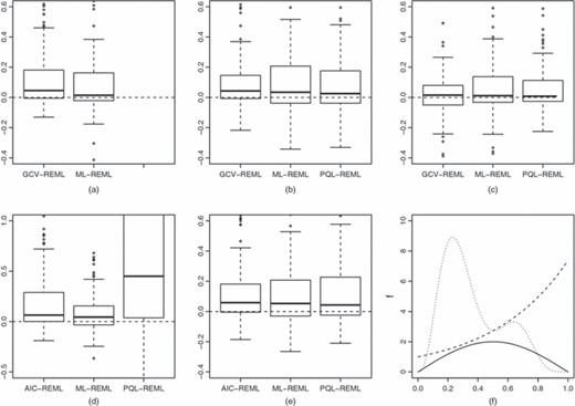
Mean-square error (MSE) comparisons between REML and other methods for five distributions: (a) normal; (b) gamma; (c) Tweedie; (d) binary; (e) Poisson; (f) components

Model performance was judged by calculating the mean-square error (MSE) in reconstructing the true linear predictor, at the observed covariate values. In the case of binary data, this measure is rather unstable for fitted probabilities in the vicinity of 0 or 1, so the probability scale was used in place of the linear predictor scale.

The results are summarized in Fig. 2. Boxplots show the distributions, over 200 replicates, of differences in MSE between each alternative method and REML. Before plotting, the MSEs are divided by the MSE for REML estimation, averaged over the the case being plotted. In all cases a Wilcoxon signed rank test indicates that REML has lower MSE than the competing method (p-value less than 10⁻³ except for the PQL–ML comparison for the Tweedie distribution where p = 0.04). The Tweedie variance power was 1.5. PQL failed in 16, 10, 22 and seven replicates, for the gamma, Tweedie, binary and Poisson data respectively. The other methods converged successfully for every replicate. The most dramatic difference is between REML and PQL for binary data, where PQL has a substantial tail of poor fits, reflecting the well-known fact that PQL is poor for binary data. Note also the skew in the GCV–REML comparisons: this seems to result from a smallish proportion of GCV- or AIC-based replicates substantially overfitting. The mean time per replicate for GCV or AIC, REML and ML was about 0.7 s on a 1.33-GHz Intel U7700 computer running LINUX (on a mid-range laptop). PQL took between 10 and 20 times longer. All computations were performed with R 2.9.2 (R Development Core Team, 2008) and R package mgcv version 1.6-1 (which includes a Tweedie family based on Dunn and Smith (2005)).

The experiment was repeated at lower noise levels: first for noise levels such that the r²-value between μ_i and y_i was about 0.7 and then for still lower noise levels so that the r²-value was about 0.95. Fig. 3 shows the results for the lowest noise level. In this case ML gives the best MSE performance, although REML is not much worse and still better than the prediction error criteria. The intermediate noise level results are not shown, but indicate ML and REML to be almost indistinguishable, and both better than prediction error criteria. It seems likely that the superiority of ML over REML in the lowest noise case relates to Wahba’s (1985) demonstration that REML undersmooths, asymptotically: ML will of course smooth more but is still consistent (Kauermann et al., 2009). Similarly the failure of prediction error methods to show any appreciable catch-up as noise levels were reduced, despite their asymptotic superiority in MSE terms, presumably relates to the excruciatingly slow convergence rates for prediction-criteria-based estimates, obtained in Härdle et al. (1988).

Fig. 3

Open in new tab Download slide

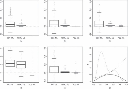
As for Fig. 2, but using data for which only 5% of the variance in the response was noise: in this case ML gave the best MSE performance and so has replaced REML as the reference method (all differences are significant at p<0.000 04 except the PQL–ML comparisons for the gamma, Tweedie and Poisson distributions for which the p-values are 0.01, 0.01 and 0.0006)

The two problematic examples from the introduction to Wood (2008), Figs 1 and 2, were also repeated with the methods that are developed here: convergence was unproblematic and reasonable fits were obtained. See Appendix A for some further comparisons with another alternative method.

The simulation evidence supports the implication of Reiss and Ogden’s (2009) work, that REML (and hence the structurally very similar ML) may have practical advantages over GCV or AIC for smoothing parameter selection, and reinforces the message from Wood (2008), that direct nested optimization is quicker and more reliable than selecting smoothing parameters on the basis of approximate working models.

5. Examples

This section presents three example applications which, as special cases of penalized GLMs, are straightforward given the general method that is proposed in this paper.

5.1. Simple P-spline adaptive smoothing

An important feature of the method proposed is that it is stable even when different penalties act on intersecting sets of parameters. Tensor product smooths that are used for smooth interaction terms are an obvious important case where this occurs (see for example Wood (2006), section 4.1.8), but adaptive smoothing provides a less-well-known example, as illustrated in this section, using adaptive P-splines.

The ‘P-splines’ of Eilers and Marx (1996) combine B-spline basis functions and discrete penalties on the basis coefficients, to obtain flexible spline-like smoothers. For example, if we let b_j(x) denote B-spline basis functions, with evenly spaced knots, then an unknown function f can be represented (approximately) as

f (x) = \sum_{i = 1}^{K} β_{i} b_{i} (x)

and the wiggliness of this function can be measured by using the discrete penalty

P_{ordinary} = \sum_{i = 2}^{K - 1} {(β_{i - 1} - 2 β_{i} + β_{i + 1})}^{2},

or higher or lower order alternatives. The penalty can be used as a smoothing penalty in fitting. One of the reasons that P-splines have proved so popular is the ease with which they can be modified to perform non-standard smoothing tasks, at relatively little loss of performance relative to more computationally complex smoothers. Adaptive smoothing illustrates this.

An adaptive penalty is easily constructed by allowing the terms in the penalty to have different weights, depending on i, and hence on x. For example:

P = \sum_{i = 2}^{K - 1} c_{i} {(β_{i - 1} - 2 β_{i} + β_{i + 1})}^{2} .

Now defining d_i = β_i−1−2β_i+β_i+1, and D to be the matrix of coefficients such that d = Dβ, we have

P = β^{T} D^{T} diag (c) D β .

The elements c_i are unknown, but we could use a B-spline basis to model the c_i as a smooth function of i or x so that c = Cλ, where λ is a vector of unknown (positive) coefficients. In this case

P = \sum_{j} λ_{j} β^{T} D^{T} diag (C \cdot, j) D β

where C_·,j is column j of C, i.e. the adaptive penalty has become a sum of penalties multiplied by smoothing parameters λ_j. The same construction can be used for smooths of several covariates, using tensor products of P-splines. See Krivobokova et al. (2008) for a more sophisticated P-spline-based approach to this problem.

The obvious advantage of the approach that is given here is that it allows adaptive smoothers to be used as components of penalized GLMs in the same way as any other smooth. As an example consider smoothing the well-known motorcycle crash data that were used in Silverman (1985). The response a_i is acceleration of the head of a test dummy in a simulated motorcycle crash, and it depends on time t_i. A simple model is

a_{i} = f (t_{i}) + ε_{i}

where the ɛ_i are IID N(0,σ²) (although a better model would have σ² depending on time as well). Given that the data show a low acceleration phase followed by rapid changes in acceleration followed by a smooth return to zero, it is possible to make the case that the degree of penalization of f should depend on t. A model was therefore fitted in which f was represented by using a rank 40 cubic B-spline basis (even knot spacing), penalized by using the adaptive penalty given above, λ having dimension 5 (although the results are rather insensitive to the exact choice here). The smoothing parameters λ were chosen by REML.

The results are shown in Fig. 4, which also includes a fit in which a single-penalty rank 40 thin plate regression spline is used to represent f(t). The single-penalty case must use the same degree of penalization for all t, with the result that the curve at low and high times appears underpenalized and too bumpy, presumably to accommodate the high degree of variability at intermediate times. The adaptive fit took 1.3 s, compared with 0.15 s for the single-penalty fit (see Section 4, for computer details).

Fig. 4

Open in new tab Download slide

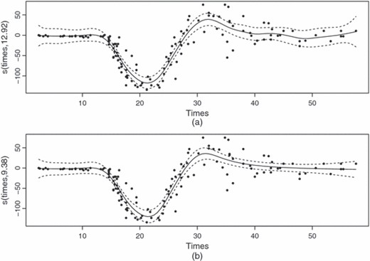
Two attempts to smooth the motorcycle crash data (all smoothing parameters were chosen by REML; note that the adaptive smoother uses fewer effective degrees of freedom and produces a fit which appears to show better adaptation to the data): (a) the smooth as a rank 40 penalized thin plate regression spline; (b) a simple adaptive smoother of the type discussed in Section 5.1

5.2. Generalized regression of scalars on functions

The fact that the method that is described in this paper has been developed for the rather general model (1) means that it can be used for models that superficially appear to be rather different from a GAM. To illustrate this, this section revisits an example from Reiss and Ogden (2009) but makes use of the new method to employ a more general model than theirs, based on non-Gaussian errors with multiple penalties.

Consider a response y_i which is dependent on predictor function z_i(x), where x may be univariate or multivariate. In this case an appropriate model might be

g (μ_{i}) = α + \int f (x) z_{i} (x) d x,

(15)

with y_i an observation from some exponential family distribution, with mean μ_i. f(x) is an unknown ‘coefficient’ function and must be estimated. It is straightforward to extend the model by adding other smooth terms to the linear predictor (the right-hand side). In practice the integral will be approximated by quadrature, with the midpoint rule being adequate in most cases. Suppose that the domain of z_i(x) is finite and let x_j denote points at which z_i has been observed (with even spacing h). The model becomes

g (μ_{i}) = α + h \sum_{j} f (x_{j}) z_{i} (x_{j}) .

Any penalized regression spline basis can be used for f, and model estimation proceeds as for any other penalized GLM. For more detail on such models see Marx and Eilers (1999), Escabias et al. (2004), Ramsay and Silverman (2005) or Reiss and Ogden (2007) (and also Wahba (1990)).

As an example, consider trying to predict the octane rating of gasoline (or petrol) from its near infrared spectrum. For internal combustion engines in which a fuel–air mixture is compressed within the cylinders before combustion, it is important that the fuel–air mixture does not spontaneously ignite owing to compressive heating. Such early combustion results in ‘knocking’ and poor engine performance. The octane rating of fuel measures its resistance to knocking. It is a somewhat indirect measure: the lowest compression ratio at which the fuel causes knocking is recorded. The octane rating is the percentage of iso-octane in the mixture of n-heptane and iso-octane with the same lowest knocking compression ratio as the fuel sample. Measuring octane rating requires special variable compression test engines, and it would be rather simpler to measure the octane from spectral measurements on a fuel sample, if this were possible.

Fig. 5(a) shows near infrared spectra for 60 gasoline samples (from Kalivas (1997), as provided by Wehrens and Mevik (2007)). The octane rating of each sample has also been measured. Model (15) is a possibility for such data (where y_i is octane rating, z_i(x) is the ith spectrum and x is wavelength). The octane rating is positive and continuous (at least in theory), and there is some indication of increasing variance with mean (see Fig. 5(c)), so a gamma distribution with log-link is an appropriate initial model. The spectra themselves are rather spiky, with some smooth regions interspersed with regions of very rapid variation. It seems sensible to allow the coefficient function f(x) the possibility of behaving in a similar way, so representing f by using the same sort of adaptive smooth as was used in the previous section is appropriate. Estimation of this model is then just a case of estimating a GLM subject to multiple penalization. The remaining panels of Fig. 5 show the results of this fitting, with REML smoothness selection.

Fig. 5

Open in new tab Download slide

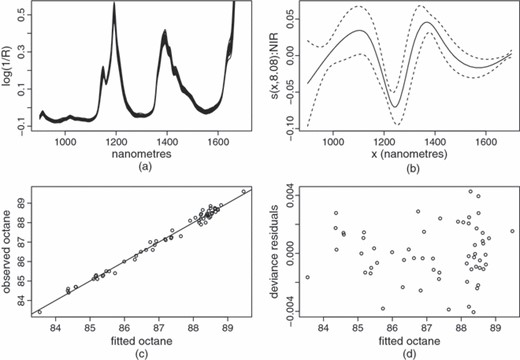
(a) Near infrared spectra for 60 samples of gasoline (the y-axis is the logarithm of the inverse of reflectance, which is measured every 2 nm; these spectra ought to be able to predict the octane rating of the samples; the spectra actually reach 1.2 at the right-hand end but, since this region turns out to have little predictive power, the y-axis has been truncated to show more detail at lower wavelengths); (b) estimated coefficient function for the model given in Section 5.2, with factor h absorbed (the inner product of this with the spectrum for a sample gives the predicted octane rating); (c) observed versus fitted ratings; (d) deviance residuals for the model versus fitted octane rating

Note that the coefficient function appears to be contrasting the two peak regions with the trough between them, with the extreme ends of the spectra apparently adding little. The model explains around 98% of the deviance in octane rating, and the residual plots look plausible (including a QQ-plot of deviance residuals, which is not shown).

5.3. Generalized additive model term selection and null space penalties

Smoothing parameter selection does most of the work in selecting between models of differing complexity, but it does not usually remove a term from the model altogether. If the smoothing parameter for a term tends to ∞, this usually causes the term to tend towards some simple, but non-zero, function of its covariate. For example, as its smoothing parameter tends to ∞, a cubic regression spline term will tend to a straight line. It seems logical to decide on whether or not terms should be included in the model by using the same criterion as used for smoothness selection, but how should this be achieved in practice? Tutz and Binder (2006) proposed one solution to the model selection problem, by using a boosting approach to perform fitting, smoothness selection and term selection simultaneously. They also provided evidence that in very data poor settings, with many spurious covariates, this approach can be much better than the alternatives. This section proposes a possible alternative to boosting, in which each smooth term is given an extra penalty, which will shrink to zero any functions that are in the null space of the usual penalty.

For example, consider a smooth with K coefficients β and penalty matrix $S$ ⁠, with null space dimension M_s, so that the wiggliness penalty is $β^{T} S β$ ⁠. Now consider the eigendecomposition $S = U Λ U^{T}$ ⁠. The first K−M_s eigenvalues Λ_i will be positive, and the last M_s will be 0. Writing Λ₊ for the (K−M_s)×(K−M_s) diagonal matrix containing only the positive eigenvalues, and U₊ for the K×(K−M_s) matrix of corresponding eigenvectors, then $S = U Λ U^{T}$ ⁠. Now let U₋ be the K×M_s matrix of the eigenvectors corresponding to zero eigenvalues. U₊ forms a basis for the space of coefficients corresponding to the ‘wiggly’ component of the smooth, whereas U₋ is a basis for the components of zero wiggliness—the null space of the penalty. The two bases are orthogonal. So, if we want to produce a penalty which penalizes only the null space of the penalty, we could use $β^{T} S_{N} β$ where $S_{N} = U_{-} U_{-}^{T}$ ⁠. If a smooth term is already subject to multiple penalties (e.g. a tensor product smooth or an adaptive smooth), the same basic construction holds, but the null space is obtained from the eigendecomposition of the sum of the original penalty matrices. Note that this construction is general and completely automatic.

This sort of construction could be used with any smoothing parameter selection method, not just REML or ML, but it is less appealing if used with a method which is prone to undersmoothing, as GCV seems to be.

As a small example, Poisson data were simulated assuming a log-link and a linear predictor made up of the sum of the three functions shown in Fig. 2(f) applied to three sets of 200 IID U(0,1) covariates. Six more IID U(0,1) nuisance covariates were simulated. A GAM was fitted to the simulated data, assuming a Poisson distribution and log-link, and with a linear predictor consisting of a sum of nine smooth functions of the nine covariates. Each smooth function was represented by using a rank 10 cubic regression spline (actually P-splines for GAM boosting). The model was fitted by using four different methods: the GAM boosting method of Tutz and Binder (2006), using version 1.1 of R package GAMBoost (with penalty set to 500 to ensure that each fit used well over the 50 boosting steps that were suggested as the minimum by Tutz and Binder (2006)); GCV smoothness selection, with the null space penalties that were suggested here, REML with no null space penalties and REML with null space penalties. 200 replicates of this experiment were run, and the MSE in the linear predictor at the covariate values was recorded for each method for each replicate.

Fig. 6 shows the results. REML with null space penalties achieves lower MSE than REML without null space penalties, and substantially better performance than GCV with null space penalties or GAM boosting. The success of the methods in identifying which components should be in the model at all was also recorded. For GAM boosting the methods given in the GAMBoost package were employed, whereas, for the null space penalties, terms with effective degrees of freedom greater than 0.2 were deemed to have been selected. On this basis the false negative selection rates (rates at which influential covariates were not selected) were 0.6% for boosting and 0.16% for the other methods. The false positive selection rates (rates at which spurious terms were selected) were 67%, 71% and 62% for boosting, GCV and REML respectively. REML with null space penalties took just under 6 s per fit, on average, whereas boosting took about 2.5 min per fit. Note that the example here has relatively high information content, relative to the scenarios that were investigated by Binder and Tutz (2006): with less information boosting is still appealing.

Fig. 6

Open in new tab Download slide

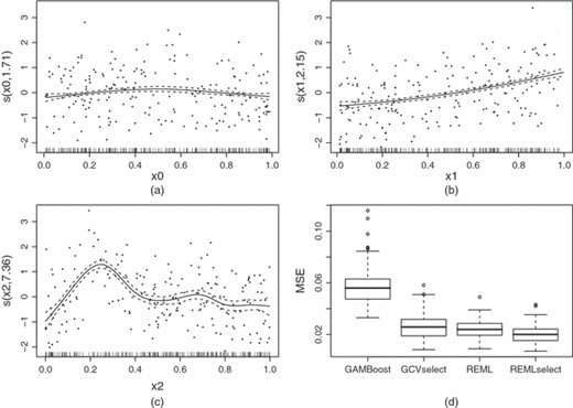
Model selection example (models were fitted to Poisson data simulated from a linear predictor made up of the three terms shown in Fig. 2(f); the linear predictors of the fitted models also included smooth functions of six additional nuisance predictors; four alternative fitting methods were used for each replicate simulation): (a)–(c) typical estimates of the terms that actually made up the true linear predictor, using REML, with selection penalties (partial Pearson residuals are shown for each smooth estimate); (d) distribution, over 200 replicates, of the MSE of the models fitted by each of the methods (‘GAMBoost’ is fitted by using Tutz and Binder’s (2006) boosting method, ‘GCVselect’ is for models with selection penalties under GCV smoothness selection, ‘REML’ is REML smoothness selection without selection penalties and ‘REMLselect’ is for REML smoothness selection with selection penalties)

6. Discussion

The method that was proposed in this paper offers a general computationally efficient way of estimating the smoothing parameters of models of the form (1), when the f_j are represented by using penalized regression splines and the coefficients β are estimated by optimizing expression (3). With this method, REML- or ML-based estimation of semiparametric GLMs can rival the estimation of ordinary parametric GLMs for routine computational reliability. Previously such efficiency and reliability were only available for prediction error criteria, such as GCV. This means that the advantages of REML or ML estimation that were outlined in Section 1.1 need no longer be balanced against the more reliable fitting methods that are available for GCV or AIC. The cost of this enhancement is that the method proposed has a somewhat more complex mathematical structure than the previous prediction-error-based methods (e.g. Wood (2008)), but since the method is freely available in R package mgcv (from version 1.5) this is not an obstacle to its use.

Given that REML or ML estimation requires that we view model (1) as a generalized linear mixed model, then an obvious question is why should it be treated as a special case for estimation purposes, rather than estimated by general generalized linear mixed model software? The answer lies in the special nature of the λ_i. The fact that they enter the penalty or precision matrix linearly, facilitates both the evaluation of derivatives to computational accuracy and the ability to stabilize the computations via the method of Appendix B. In addition the λ_i are unusual precision parameters in that their ‘true’ value is often infinite. This behaviour can cause problems for general purpose methods, which cannot exploit the advantages of the linear structure. Conversely, the method that is proposed here can be used to fit any generalized linear mixed model where the precision matrix is a linear combination of known matrices but, since it is not designed to exploit the sparse structure that many random effects have, it may not be the most efficient method for so doing.

A limitation of the method that was presented here is that it is designed to be efficient when the f_j are represented by using penalized regression splines as described in Wahba (1980), Parker and Rice (1985), Eilers and Marx (1996), Marx and Eilers (1998), Ruppert et al. (2003), Wood (2003) etc. These ‘intermediate rank’ smoothers have become very popular over the last decade, as researchers realized that many of the advantages of splines could be obtained without the computational expense of full splines: an opinion which turns out to be well founded theoretically (see Gu and Kim (2002), Hall and Opsomer (2005) and Kauermann et al. (2009)). But, despite its wide applicability, the penalized regression spline approach has limitations. The most obvious is that relatively low rank smooths are unsuitable for modelling short-range auto-correlation (particularly spatial). Where this deficiency matters, Rue et al. (2009) offer an attractive alternative approach, by directly estimating additive smooth components of the linear predictor, with very sparse S_j-matrices directly penalizing these components. The required sparsity can be obtained by modelling the smooth components as Markov random fields of some sort. Provided that the number of smoothing parameters is quite low, then the methods offer very efficient computation for this class of problem, as well as better inferences about the smoothing parameters themselves. When the model includes large numbers of random effects, but not all components have the sparsity that is required by Rue et al. (2009), or when the number of smoothing parameters or variance parameters is moderate to large, then the simulation-based Bayesian approach of Fahrmeir, Lang and co-workers (e.g. Lang and Brezger (2004), Brezger and Lang (2006) and Fahrmeir and Lang (2001)) is likely to be more efficient than the method that is proposed here, albeit applicable to a more restricted range of penalized GLMs, because of restrictions on the S_j that are required to maintain computational efficiency.

An interesting area for further work would be to establish relative convergence rates for the ${\hat{f}}_{j}$ under REML, ML and GCV smoothness selection. It is not difficult to arrange for ${\hat{f}}_{j}$ to be consistent under either approach, at least when spline-like bases are used for the f_j in model (1). Without penalization, all that we require is that the basis dimension grows with sample size n sufficiently fast that the spline approximation error declines at a faster rate than the sampling variance of ${\hat{f}}_{j}$ ⁠, but sufficiently slow that dim(β)/n→0 (so that the observed likelihood converges to its expectation). This is not difficult to achieve, given the good approximation theoretic properties of splines. If smoothing parameters are chosen to be sufficiently small, then penalization will reduce the MSE at any n, so consistency can be maintained under penalized estimation. In fact, asymptotically, GCV minimizes the MSE (or a generalized equivalent), so the ${\hat{f}}_{j}$ will be consistent under GCV estimation. Since REML smooths less than GCV, asymptotically (Wahba, 1985), then the same must hold for REML. However, establishing the relative convergence rates that are actually achieved under the two alternatives appears to be more involved.

Acknowledgements

I am especially grateful to Mark Bravington for explanation of the implicit function theorem, and for providing the original fisheries modelling examples that broke Fisher-scoring-based approaches, and to Phil Reiss for first alerting me to the real practical advantages of REML and providing an early preprint of Reiss and Ogden (2009). The Commonwealth Scientific and Industrial Research Organisation paid for a visit to Hobart where the Tweedie work was done, and it became clear that the Wood (2008) method could not be extended to REML. Thanks also go to Mark Bravington, Merrilee Hurn and Alistair Spence for some helpful discussions during the painful process that led to the Section 3.1– Appendix B method. Phil Reiss, Mark Bravington, Nicole Augustin and Giampiero Marra all provided very helpful comments on an earlier draft of this paper. The Joint Editor, Associate Editor and two referees all made suggestions which substantially improved the paper, for which I am also grateful.

References

Anderson

,

E.

,

Bai

,

Z.

,

Bischof

,

C.

,

Blackford

,

S.

,

Demmel

,

J.

,

Donngarra

,

J.

,

Du Croz

,

J.

,

Greenbaum

,

A.

,

Hammerling

,

S.

,

McKenney

,

A.

and

Sorenson

,

D.

(

1999

)

LAPACK Users’ Guide

, 3rd edn.

Philadelphia

:

Society for Industrial and Applied Mathematics

.

Anderssen

,

R. S.

and

Bloomfield

,

P.

(

1974

)

A time series approach to numerical differentiation

.

Technometrics

,

16

,

69

–

75

.

Google Scholar

Crossref

WorldCat

Breslow

,

N. E.

and

Clayton

,

D. G.

(

1993

)

Approximate inference in generalized linear mixed models

.

J. Am. Statist. Ass.

,

88

,

9

–

25

.

Google Scholar

OpenURL Placeholder Text

WorldCat

Brezger

,

A.

,

Kneib

,

T.

and

Lang

,

S.

(

2007

)

BayesX 1.5.0

.

University of Munich

,

Munich

. (Available from http://www.stat.uni-muenchen.de/~bayesx.)

Brezger

,

A.

and

Lang

,

S.

(

2006

)

Generalized structured additive regression based on Bayesian P-splines

.

Computnl Statist. Data Anal.

,

50

,

967

–

991

.

Google Scholar

Crossref

WorldCat

Cline

,

A. K.

,

Moler

,

C. B.

,

Stewart

,

G. W.

and

Wilkinson

,

J. H.

(

1979

)

An estimate for the condition number of a matrix

.

SIAM J. Numer. Anal.

,

13

,

293

–

309

.

Google Scholar

Crossref

WorldCat

Craven

,

P.

and

Wahba

,

G.

(

1979

)

Smoothing noisy data with spline functions: estimating the correct degree of smoothing by the method of generalized cross validation

.

Numer. Math.

,

31

,

377

–

403

.

Google Scholar

Crossref

WorldCat

Davison

,

A. C.

(

2003

)

Statistical Models

.

Cambridge

:

Cambridge University Press

.

Demidenko

,

E.

(

2004

)

Mixed Models: Theory and Applications

.

Hoboken

:

Wiley

.

Dunn

,

P. K.

and

Smith

,

G. K.

(

2005

)

Series evaluation of Tweedie exponential dispersion model densities

.

Statist. Comput.

,

15

,

267

–

280

.

Google Scholar

Crossref

WorldCat

Efron

,

B.

and

Hinkley

,

D. V.

(

1978

)

Assessing the accuracy of the maximum likelihood estimator: observed versus expected Fisher information

.

Biometrika

,

65

,

457

–

487

.

Google Scholar

Crossref

WorldCat

Eilers

,

P. H. C.

and

Marx

,

B. D.

(

1996

)

Flexible smoothing with B-splines and penalties

.

Statist. Sci.

,

11

,

89

–

121

.

Google Scholar

Crossref

WorldCat

Eilers

,

P. H. C.

and

Marx

,

B. D.

(

2002

)

Generalized linear additive smooth structures

.

J. Computnl Graph. Statist.

,

11

,

758

–

783

.

Google Scholar

Crossref

WorldCat

Escabias

,

M.

,

Aguilera

,

A. M.

and

Valderrama

,

M. J.

(

2004

)

Principal component estimation of functional logistic regression: discussion of two different approaches

.

Nonparam. Statist.

,

16

,

365

–

384

.

Google Scholar

Crossref

WorldCat

Fahrmeir

,

L.

,

Kneib

,

T.

and

Lang

,

S.

(

2004

)

Penalized structured additive regression for space time data: a Bayesian perspective

.

Statist. Sin.

,

14

,

731

–

761

.

Google Scholar

OpenURL Placeholder Text

WorldCat

Fahrmeir

,

L.

and

Lang

,

S.

(

2001

)

Bayesian inference for generalized additive mixed models based on Markov random field priors

.

Appl. Statist.

,

50

,

201

–

220

.

Google Scholar

OpenURL Placeholder Text

WorldCat

Golub

,

G. H.

and

van Loan

,

C. F.

(

1996

)

Matrix Computations

, 3rd edn.

Baltimore

:

Johns Hopkins University Press

.

Google Scholar

Google Preview

OpenURL Placeholder Text

WorldCat

Green

,

P. J.

and

Silverman

,

B. W.

(

1994

)

Nonparametric Regression and Generalized Linear Models

.

London

:

Chapman and Hall

.

Gu

,

C.

(

1992

)

Cross validating non-Gaussian data

.

J. Computnl Graph. Statist.

,

1

,

169

–

179

.

Google Scholar

OpenURL Placeholder Text

WorldCat

Gu

,

C.

(

2002

)

Smoothing Spline ANOVA Models

.

New York

:

Springer

.

Gu

,

C.

and

Kim

,

Y.-J.

(

2002

)

Penalized likelihood regression: general formulation and efficient approximation

.

Can. J. Statist.

,

30

,

619

–

628

.

Google Scholar

Crossref

WorldCat

Hall

,

P.

and

Opsomer

,

J. D.

(

2005

)

Theory for penalised spline regression

.

Biometrika

,

92

,

105

–

118

.

Google Scholar

Crossref

WorldCat

Härdle

,

W.

,

Hall

,

P.

and

Marron

,

J. S.

(

1988

)

How far are automatically chosen regression smoothing parameters from their optimum?

J. Am. Statist. Ass.

,

83

,

86

–

95

.

Google Scholar

OpenURL Placeholder Text

WorldCat

Harville

,

D. A.

(

1977

)

Maximum likelihood approaches to variance component estimation and to related problems

.

J. Am. Statist. Ass.

,

72

,

320

–

338

.

Google Scholar

Crossref

WorldCat

Harville

,

D. A.

(

1997

)

Matrix Algebra from a Statistician’s Perspective

.

New York

:

Springer

.

Hastie

,

T.

and

Tibshirani

,

R.

(

1986

)

Generalized additive models (with discussion)

.

Statist. Sci.

,

1

,

297

–

318

.

Google Scholar

OpenURL Placeholder Text

WorldCat

Hastie

,

T.

and

Tibshirani

,

R.

(

1990

)

Generalized Additive Models

.

London

:

Chapman and Hall

.

Google Scholar

Google Preview

OpenURL Placeholder Text

WorldCat

Hastie

,

T.

and

Tibshirani

,

R.

(

1993

)

Varying-coefficient models (with discussion)

.

J. R. Statist. Soc. B

,

55

,

757

–

796

.

Google Scholar

OpenURL Placeholder Text

WorldCat

Hurvich

,

C. M.

,

Simonoff

,

J. S.

and

Tsai

,

C.-L.

(

1998

)

Smoothing parameter selection in nonparametric regression using an improved Akaike information criterion

.

J. R. Statist. Soc. B

,

60

,

271

–

293

.

Google Scholar

Crossref

WorldCat

Kalivas

,

J. H.

(

1997

)

Two data sets of near infrared spectra

.

Chemometr. Intell. Lab. Syst.

,

37

,

255

–

259

.

Google Scholar

Crossref

WorldCat

Kauermann

,

G.

(

2005

)

A note on smoothing parameter selection for penalized spline smoothing

.

J. Statist. Planng Inf.

,

127

,

53

–

69

.

Google Scholar

Crossref

WorldCat

Kauermann

,

G.

,

Krivobokova

,

T.

and

Fahrmeir

,

L.

(

2009

)

Some asymptotic results on generalized penalized spline smoothing

.

J. R. Statist. Soc. B

,

71

,

487

–

503

.

Google Scholar

Crossref

WorldCat

Kimeldorf

,

G.

and

Wahba

,

G.

(

1970

)

A correspondence between Bayesian estimation of stochastic processes and smoothing by splines

.

Ann. Math. Statist.

,

41

,

495

–

502

.

Google Scholar

Crossref

WorldCat

Kohn

,

R.

,

Ansley

,

C. F.

and

Tharm

,

D.

(

1991

)

The performance of cross-validation and maximum likelihood estimators of spline smoothing parameters

.

J. Am. Statist. Ass.

,

86

,

1042

–

1050

.

Google Scholar

Crossref

WorldCat

Krivobokova

,

T.

,

Crainiceanu

,

C. M.

and

Kauermann

,

G.

(

2008

)

Fast adaptive penalized splines

.

J. Computnl Graph. Statist.

,

17

,

1

–

20

.

Google Scholar

Crossref

WorldCat

Laird

,

N. M.

and

Ware

,

J. H.

(

1982

)

Random-effects models for longitudinal data

.

Biometrics

,

38

,

963

–

974

.

Lang

,

S.

and

Brezger

,

A.

(

2004

)

Bayesian P-splines

.

J. Computnl Graph. Statist.

,

13

,

183

–

212

.

Google Scholar

Crossref

WorldCat

Marx

,

B. D.

and

Eilers

,

P. H.

(

1998

)

Direct generalized additive modeling with penalized likelihood

.

Computnl Statist. Data Anal.

,

28

,

193

–

209

.

Google Scholar

Crossref

WorldCat

Marx

,

B. D.

and

Eilers

,

P. H.

(

1999

)

Generalized linear regression on sampled signals and curves: a P-spline approach

.

Technometrics

,

41

,

1

–

13

.

Google Scholar

Crossref

WorldCat

Monahan

,

J. F.

(

2001

)

Numerical Methods of Statistics

.

Cambridge

:

Cambridge University Press

.

Nelder

,

J. A.

and

Wedderburn

,

R. W. M.

(

1972

)

Generalized linear models

.

J. R. Statist. Soc. A

,

135

,

370

–

384

Google Scholar

Crossref

WorldCat

Nocedal

,

J.

and

Wright

,

S. J.

(

2006

)

Numerical Optimization

, 2nd edn.

New York

:

Springer

.

Google Scholar

Google Preview

OpenURL Placeholder Text

WorldCat

Parker

,

R. L.

and

Rice

,

J. A.

(

1985

)

Discussion on ‘Some aspects of the spline smoothing approach to non-parametric regression curve fitting’ (by B. W. Silverman)

.

J. R. Statist. Soc. B

,

47

,

40

–

42

.

Google Scholar

OpenURL Placeholder Text

WorldCat

Patterson

,

H. D.

and

Thompson

,

R.

(

1971

)

Recovery of interblock information when block sizes are unequal

.

Biometrika

,

58

,

545

–

554

.

Google Scholar

Crossref

WorldCat

Ramsay

,

J. O.

and

Silverman

,

B. W.

(

2005

)

Functional Data Analysis

.

New York

:

Springer

.

R Development Core Team

(

2008

)

R 2.8.1: a Language and Environment for Statistical Computing

.

Vienna

:

R Foundation for Statistical Computing

.

Google Scholar

Google Preview

OpenURL Placeholder Text

WorldCat

Reiss

,

P. T.

and

Ogden

,

R. T.

(

2007

)

Functional principal component regression and functional partial least squares

.

J. Am. Statist. Ass.

,

102

,

984

–

996

.

Google Scholar

Crossref

WorldCat

Reiss

,

P. T.

and

Ogden

,

R. T.

(

2009

)

Smoothing parameter selection for a class of semiparametric linear models

.

J. R. Statist. Soc. B

,

71

,

505

–

523

.

Google Scholar

Crossref

WorldCat

Rue

,

H.

,

Martino

,

S.

and

Chopin

,

N.

(

2009

)

Approximate Bayesian inference for latent Gaussian models by using integrated nested Laplace approximations (with discussion)

.

J. R. Statist. Soc. B

,

71

,

319

–

392

.

Google Scholar

Crossref

WorldCat

Ruppert

,

D.

,

Wand

,

M. P.

and

Carroll

,

R. J.

(

2003

)

Semiparametric Regression

.

Cambridge

:

Cambridge University Press

.

Silverman

,

B. W.

(

1985

)

Some aspects of the spline smoothing approach to non-parametric regression curve fitting (with discussion)

.

J. R. Statist. Soc. B

,

47

,

1

–

52

.

Google Scholar

OpenURL Placeholder Text

WorldCat

Tutz

,

G.

and

Binder

,

H.

(

2006

)

Generalized additive modeling with implicit variable selection by likelihood-based boosting

.

Biometrics

,

62

,

961

–

971

.

Tweedie

,

M. C. K.

(

1984

) An index which distinguishes between some important exponential families. In

Statistics: Applications and New Directions: Proc. Indian Statistical Institute Golden Jubilee Int. Conf

. (eds

J. K.

Ghosh

and

J.

Roy

), pp.

579

–

604

.

Calcutta

:

Indian Statistical Institute

.

Google Scholar

Google Preview

OpenURL Placeholder Text

WorldCat

Venables

,

W. N.

and

Ripley

,

B. D.

(

2002

)

Modern Applied Statistics with S

, 4th edn.

New York

:

Springer

.

Wahba

,

G.

(

1980

) Spline bases, regularization and generalized cross validation for solving approximation problems with large quantities of noisy data. In

Approximation Theory III

(ed.

E.

Cheney

).

London

:

Academic Press

.

Google Scholar

Google Preview

OpenURL Placeholder Text

WorldCat

Wahba

,

G.

(

1983

)

Bayesian ‘‘confidence intervals’’ for the cross-validated smoothing spline

.

J. R. Statist. Soc. B

,

45

,

133

–

150

.

Google Scholar

OpenURL Placeholder Text

WorldCat

Wahba

,

G.

(

1985

)

A comparison of GCV and GML for choosing the smoothing parameter in the generalized spline smoothing problem

.

Ann. Statist.

,

13

,

1378

–

1402

.

Google Scholar

OpenURL Placeholder Text

WorldCat

Wahba

,

G.

(

1990

)

Spline Models for Observational Data

.

Philadelphia

:

Society for Industrial and Applied Mathematics

.

Wahba

,

G.

and

Wold

,

S.

(

1975

)

A completely automatic French curve: fitting spline functions by cross-validation

.

Communs Statist. Theor. Meth.

,

4

,

125

–

141

.

Google Scholar

OpenURL Placeholder Text

WorldCat

Watkins

,

D. S.

(

1991

)

Fundamentals of Matrix Computations

.

New York

:

Wiley

.

Google Scholar

Google Preview

OpenURL Placeholder Text

WorldCat

Wehrens

,

R.

and

Mevik

,

B.-H.

(

2007

) pls: Partial Least Squares Regression (PLSR) and Principal Component Regression (PCR).

R Package Version 2.1-0

. (Available from http://mevik.net/work/software/pls.html.)

Google Scholar

Google Preview

OpenURL Placeholder Text

WorldCat

Wood

,

S. N.

(

2003

)

Thin plate regression splines

.

J. R. Statist. Soc. B

,

65

,

95

–

114

.

Google Scholar

Crossref

WorldCat

Wood

,

S. N.

(

2004

)

Stable and efficient multiple smoothing parameter estimation for generalized additive models

.

J. Am. Statist. Ass.

,

99

,

673

–

686

.

Google Scholar

Crossref

WorldCat

Wood

,

S. N.

(

2006

)

Generalized Additive Models: an Introduction with R

.

Boca Raton

:

CRC–Chapman and Hall

.

Wood

,

S. N.

(

2008

)

Fast stable direct fitting and smoothness selection for generalized additive models

.

J. R. Statist. Soc. B

,

70

,

495

–

518

.

Google Scholar

Crossref

WorldCat

Appendix A: Convergence failures of previous restricted maximum likelihood schemes

Wood (2008) provides some examples of convergence failure for the PQL approach, in which smoothing parameters are estimated iteratively by REML or ML estimation of working linear mixed models. The alternative scheme that is proposed in the literature has been implemented by Brezger et al. (2007) in the BayesX package. Like PQL, this scheme need not converge (as Brezger et al. (2007) explicitly pointed out), but Brezger et al. (2007) employed an ingenious heuristic stabilization trick which seems to lead to superior performance to that of PQL in this regard. However, it is not difficult to find realistic examples that still give convergence problems. For example the following code was used in R version 2.7.1 to generate data with a relatively benign collinearity problem and a mild mean–variance relationship problem:

\begin{array}{l} set . seed (1); n < - 1000; alpha < - .75 \\ x 0 < - runif (n); x 1 < - x 0 * alpha + (1 - alpha) * runif (n) \\ x 2 < - runif (n); x 3 < - x 2 * alpha + (1 - alpha) * runif (n) \\ x 4 < - runif (n); x 5 < - runif (n) \\ f 0 < - function (x) 2 * \sin (p i * x) \\ f1 < - function (x) exp (2 * x) \\ f2 < -function (x) 0.2 * x^{\land} 11 * (10 * (1 - x)) \land 6 + 10 * (10 * x) \land 3 * (1 - x) \land 10 \\ f<-f 0(x 0)+f 1(x 1)+f 2(x 2) \\ y < - rgamma (f, \exp (f / 4), scale = 1.2) \end{array}

Fitting the model

\log \{E (y_{i})\} = f_{1} (x_{1 i}) + f_{2} (x_{2 i}) + f_{3} (x_{3 i}) + f_{4} (x_{4 i}) + f_{5} (x_{5 i}) + f_{6} (x_{6 i}),

y_i∼ gamma, in BayesX version 1.5.0, representing each f by a (default) rank 20 P-spline, resulted in convergence failure, with the estimates zigzagging without ever converging. Nine subsequent replicates of this experiment yielded two more convergence failures of the same sort, three catastrophic divergences and four problem-free convergences (although one of these took more than 200 iterations). Fitting the same model to these data sets by using the methods that are proposed in this paper gave no problems and sensible function reconstructions in each case.

Appendix B: |∑_iλ_iS_i|₊

As discussed in Section 3.1, a stable method for calculating log (|Σ_i λ_iS_i|₊) and its derivatives with respect to ρ_i = log (λ_i) is required, when the λ_i may be wildly different in magnitude. This appendix provides such a method by extending the simple approach that was described in Section 3.1.

Here it is assumed that q×q matrix S=Σ_i λ_iS_i is formally of full rank. When this is not so then the following initial transformation will be required. First form the symmetric eigendecomposition:

\tilde{U} \tilde{Λ} {\tilde{U}}^{T} = \sum_{i} S_{i} / {‖S_{i}‖}_{F},

where ‖·‖_F is the Frobenius norm. Now let U₊ denote the columns of

\tilde{U}

corresponding to positive eigenvalues. The transformation

{\tilde{S}}_{i} = U_{+}^{T} S_{i} U_{+}

is then applied and the methods of this appendix are utilized on the transformed matrices. It is easy to show that

| S |_{+} = |Σ_{i} λ_{i} {\tilde{S}}_{i}|

⁠, and that

Σ_{i} λ_{i} {\tilde{S}}_{i}

has full rank. For the rest of this appendix it is assumed that this transformation has been applied if necessary, and the tildes are dropped.

Initialization: set K = 0, Q = q and ${\bar{S}}_{i} = S_{i}, \forall i$ ⁠. Set γ = {1…M}, where M is the number of S_i-matrices.

Similarity transformation: the following steps are iterated until the termination criterion is met (at step 4).

Step 1: set $Ω_{i} = {‖{\bar{S}}_{i}‖}_{F} λ_{i}, \forall i \in γ$ ⁠.
Step 2: create α = {i:Ω_i⩾ɛ max(Ω_i),i ∈ γ} and γ^′={i:Ω_i<ɛ max(Ω_i),i ∈ γ} where ɛ is, for example, the cube root of the machine precision. So α indexes the dominant terms out of those remaining.
Step 3: find the eigenvalues of $Σ_{i \in α} {\bar{S}}_{i} / {‖{\bar{S}}_{i}‖}_{F}$ and use these to determine the formal rank r of any summation of the form $Σ_{i \in α} λ_{i} {\bar{S}}_{i}$ where the λ_i are positive. The rank is determined by counting the number of eigenvalues that are larger than ɛ times the dominant eigenvalue. ɛ is typically the machine precision raised to a power in [0.7,0.9].
Step 4: if r = Q then terminate. The current S is the S to use for determinant calculation.
Step 5: find the eigendecomposition $U D U^{T} = Σ_{i \in α} λ_{i} {\bar{S}}_{i}$ ⁠, where the eigenvalues are arranged in descending order on the leading diagonal of D. Let U_r be the first r columns of U and U_n the remaining columns.
Step 6: write S in partitioned form
$S = (\begin{array}{l} A_{K \times K} & B_{K \times Q} \\ B_{Q \times K}^{T} & C_{Q \times Q} \end{array})$
where the subscripts denote dimensions (rows × columns). Then set B^′ = BU and
$C^{'} = (\begin{matrix} D_{r} + U_{r}^{T} S_{γ^{'}} U_{r} & U_{r}^{T} S_{γ^{'}} U_{n} \\ U_{n}^{T} S_{γ^{'}} U_{r} & U_{n}^{T} S_{γ^{'}} U_{n} \end{matrix})$
where $S_{γ^{'}} = Σ_{i \in γ^{'}} λ_{i} {\bar{S}}_{i}$ ⁠. Then
$S^{'} = (\begin{matrix} I_{K} & 0 \\ 0 & U^{T} \end{matrix}) S (\begin{matrix} I_{K} & 0 \\ 0 & U \end{matrix}) = (\begin{matrix} A & B^{'} \\ B^{'} & C^{'} \end{matrix})$
and |S|=|S^′|. The key point here is that the effect of the terms that are indexed by α has been concentrated into an r×r block, with rows and columns to the lower right of that block uncontaminated by ‘large machine 0s’ from the terms indexed by α.
Step 7: define
$\begin{matrix} T_{α} = (\begin{matrix} I_{K} & 0 & 0 \\ 0 & U_{r} & 0 \end{matrix}), \\ T_{γ^{'}} = (\begin{matrix} I_{K} & 0 \\ 0 & U \end{matrix}) \end{matrix}$
and transform
$S_{i} \leftarrow T_{α}^{T} S_{i} T_{α} \forall i \in α$
and
$S_{i} \leftarrow T_{γ^{'}}^{T} S_{i} T_{γ^{'}} \forall i \in γ^{'} .$
These transformations facilitate derivative calculations using the transformed S.
Step 8: transform ${\bar{S}}_{i} \leftarrow U_{n}^{T} {\bar{S}}_{i} U_{n}, \forall i \in γ^{'}$ ⁠.
Step 9: set K←K+r, Q←Q−r, S←S^′ and γ←γ^′. Return to step 1.

Note that the orthogonal matrix which similarity transforms the original S to the final transformed version can be accumulated as the algorithm progresses, to produce the Q_s of Section 3.1.

The effect of the preceding iteration is to concentrate the dominant terms in S into the smallest possible block of leftmost columns, with these terms having no effect beyond those columns. Next the most dominant terms in the remainder are concentrated in the smallest possible number of immediately succeeding columns, again with no effect to the right of these columns. This pattern is repeated. Since QR-decomposition operates on columns of S, without mixing columns, it can now be used to evaluate stably the determinant of the transformed S. Alternative methods of determinant calculation (e.g. Choleski or symmetric eigendecomposition) would require an additional preconditioning step.

It is straightforward to obtain a stable matrix square root of the transformed S, which maintains the column separation that is evident in S itself. Defining diagonal matrix P_ii = |S_ii|^1/2, form the Choleski factor of the diagonally preconditioned version of S, i.e.

L L^{T} = P^{- 1} S P^{- 1} .

Then E = L^TP is a matrix square root, such that E^TE = S. Preconditioning is essential to ensure that the square root is computable without ever requiring numerical truncation, since the latter would cause spurious discontinuous changes in the numerical value of |X^TWX+S|, which depends on E.

Finally, note that, on the basis of the general results,

\frac{\partial \log | F |}{\partial x_{j}} = tr (F^{- 1} \frac{\partial F}{\partial x_{j}})

(16)

and

\frac{\partial^{2} \log | F |}{\partial x_{i} \partial x_{j}} = tr (F^{- 1} \frac{\partial^{2} F}{\partial x_{i} \partial x_{j}}) - tr (F^{- 1} \frac{\partial F}{\partial x_{i}} F^{- 1} \frac{\partial F}{\partial x_{j}})

(17)

(see Harville (1997)), the expressions for the derivatives are as follows (all right-hand side terms are transformed versions):

\frac{\partial \log | S |}{\partial ρ_{j}} = λ_{j} tr (S^{- 1} S_{j})

and

\frac{\partial^{2} \log | S |}{\partial ρ_{i} \partial ρ_{j}} = δ_{j}^{i} λ_{i} tr (S^{- 1} S_{i}) - λ_{i} λ_{j} tr (S^{- 1} S_{i} S^{- 1} S_{j}) .

Appendix C: Derivatives of $\hat{β}$ by using implicit differentiation

When full Newton optimization is used in place of Fisher scoring to obtain $\hat{β}$ ⁠, then there is no computational advantage in iterating for the derivatives of $\hat{β}$ with respect to ρ (as in Wood (2008)), rather than exploiting the implicit function theorem to obtain them directly by implicit differentiation. This is because Newton-based PIRLS requires exactly the same quantities as implicit differentiation. This appendix provides the details.

Define

D_{p} = D (β) + \sum_{m} \exp (ρ_{m}) β^{T} S_{m} β,

and note that in this appendix some care must be taken to distinguish total derivatives of D_p, which encompass all variability with respect to a variable, as opposed to partial derivatives of the expression for D_p, which ignore dependence of

\hat{β}

on ρ.

C.1. Partial derivatives of D_p

\begin{matrix} \frac{\partial D}{\partial β_{r}} = - 2 \sum_{i} ω_{i} \frac{y - μ_{i}}{V (μ_{i}) g^{'} (μ_{i})} X_{i r}, \\ \frac{d μ_{i}}{d β_{r}} = \frac{X_{i r}}{g^{'} (μ_{i})}, \end{matrix}

from which it follows (after some calculation) that

\frac{\partial^{2} D}{\partial β_{r} \partial β_{m}} = \sum_{i} 2 w_{i} X_{i m} X_{i r}

where w_i is the Newton version. Consequently

\frac{\partial^{3} D}{\partial β_{r} \partial β_{m} \partial β_{l}} = \sum_{i} \frac{d w_{i}}{d η_{i}} X_{i m} X_{i r} X_{i l} .

Note that the partials of D with respect to ρ are 0.

Turning to P = Σ_m exp (ρ_m)β^TS_mβ (so D_p = D+P) we have

\begin{matrix} \nabla_{β} P = 2 \sum_{m} \exp (ρ_{m}) S_{m} β, \\ \nabla_{β}^{2} P = 2 \sum_{m} \exp (ρ_{m}) S_{m} . \end{matrix}

Furthermore

\begin{matrix} \frac{\partial \nabla_{β} P}{\partial ρ_{j}} = 2 \exp (ρ_{j}) S_{j} β, \\ \frac{\partial^{2} \nabla_{β} P}{\partial ρ_{j} \partial ρ_{k}} = 2 δ_{j}^{k} \exp (ρ_{j}) S_{j} β, \\ \frac{\partial \nabla_{β}^{2} P}{\partial ρ_{j}} = 2 \exp (ρ_{j}) S_{j} . \end{matrix}

C.2. Derivatives of $\hat{β}$ with respect to ρ

\hat{β}

is the solution to

\frac{d D_{p}}{d β_{r}} = 0.

Since this equation always holds at

\hat{β}

⁠, we have

\frac{d^{2} D_{p}}{d β_{r} d ρ_{j}} = \sum_{m} \frac{\partial^{2} D_{p}}{\partial β_{r} \partial β_{m}} \frac{d β_{m}}{d ρ_{j}} + \frac{\partial^{2} D_{p}}{\partial β_{r} \partial ρ_{j}} = 0,

at

\hat{β}

⁠, i.e.

\frac{d \hat{β}}{d ρ_{j}} = - {(\frac{\partial^{2} D_{p}}{\partial β \partial β^{T}})}^{- 1} \frac{\partial \nabla_{β} D_{p}}{\partial ρ_{j}} .

Differentiating again we obtain

\begin{array}{l} \frac{d^{3} D_{p}}{d β_{r} d ρ_{j} d ρ_{k}} = \sum_{l} \sum_{m} \frac{\partial^{3} D_{p}}{\partial β_{r} \partial β_{m} \partial β_{l}} \frac{d β_{m}}{d ρ_{j}} \frac{d β_{l}}{d ρ_{k}} + \sum_{m} \frac{\partial^{3} D_{p}}{\partial β_{r} \partial β_{m} \partial ρ_{k}} \frac{d \hat{β}}{d ρ_{j}} + \sum_{m} \frac{\partial^{2} D_{p}}{\partial β_{r} \partial β_{m}} \frac{d^{2} β_{m}}{d ρ_{j} d ρ_{k}} \\ + \sum_{m} \frac{\partial^{3} D_{p}}{\partial β_{r} \partial β_{m} \partial ρ_{j}} \frac{d \hat{β}}{d ρ_{k}} + \frac{\partial^{3} D_{p}}{\partial β_{r} \partial ρ_{j} \partial ρ_{k}} = 0. \end{array}

Now

\frac{d η}{d ρ_{j}} = X \frac{d β}{d ρ_{j}},

so using the expression for the third partial of D/D_p with respect to ρ and rearranging we obtain

\begin{matrix} \frac{d^{2} \hat{β}}{d ρ_{j} d ρ_{k}} = - {(\frac{\partial^{2} D_{p}}{\partial β \partial β^{T}})}^{- 1} \{\frac{\partial^{2} \nabla_{β} D_{p}}{\partial ρ_{j} \partial ρ_{k}} + X^{T} f^{j k} + 2 \exp (ρ_{j}) S_{j} \frac{d \hat{β}}{d ρ_{k}} + 2 \exp (ρ_{k}) S_{k} \frac{d \hat{β}}{d ρ_{j}}\} \\ = δ_{j}^{k} \frac{d \hat{β}}{d ρ_{k}} - {(\frac{\partial^{2} D_{p}}{\partial β \partial β^{T}})}^{- 1} \{X^{T} f^{j k} + 2 \exp (ρ_{j}) S_{j} \frac{d \hat{β}}{d ρ_{k}} + 2 \exp (ρ_{k}) S_{k} \frac{d \hat{β}}{d ρ_{j}}\} \end{matrix}

where

f_{i}^{j k} = \frac{d η_{i}}{d ρ_{j}} \frac{d η_{i}}{d ρ_{k}} \frac{d w_{i}}{d η_{i}} .

The inverse required is PP^T/2 (with derivatives of dropped parameters set to 0 by this choice).

Appendix D: Derivatives of w

In this appendix primes denote differentiation with respect to μ_i. First the derivatives of α_i are useful:

α_{i}^{'} = - (\frac{V_{i}^{'}}{V_{i}} + \frac{g_{i}^{''}}{g_{i}^{'}}) + (y_{i} - μ_{i}) (\frac{V_{i}^{''}}{V_{i}} - \frac{V_{i}^{' 2}}{V_{i}^{2}} + \frac{g_{i}^{'''}}{g_{i}^{'}} - \frac{g_{i}^{'' 2}}{g_{i}^{' 2}})

and

α_{i}^{''} = - 2 (\frac{V_{i}^{''}}{V_{i}} - \frac{V_{i}^{' 2}}{V_{i}^{2}} + \frac{g_{i}^{'''}}{g_{i}^{'}} - \frac{g_{i}^{'' 2}}{g_{i}^{' 2}}) + (y_{i} - μ_{i}) (\frac{V_{i}^{'''}}{V_{i}} - \frac{3 V_{i}^{'} V_{i}^{''}}{V_{i}^{2}} + \frac{2 V_{i}^{' 3}}{V_{i}^{3}} + \frac{g_{i}^{''''}}{g_{i}^{'}} - \frac{3 g_{i}^{'''} g_{i}^{''}}{g_{i}^{' 2}} + \frac{2 g_{i}^{'' 3}}{g_{i}^{' 3}}) .

The key derivatives of w_i are then

\frac{d w_{i}}{d η_{i}} = \frac{w_{i}}{g_{i}^{'}} (\frac{α_{i}^{'}}{α_{i}} - \frac{V_{i}^{'}}{V_{i}} - 2 \frac{g_{i}^{''}}{g_{i}^{'}})

and

\frac{d^{2} w_{i}}{d η_{i}^{2}} = \frac{1}{w_{i}} {(\frac{d w_{i}}{d η_{i}})}^{2} - \frac{d w_{i}}{d η_{i}} \frac{g_{i}^{''}}{g_{i}^{' 2}} + \frac{w_{i}}{g_{i}^{' 2}} (\frac{α_{i}^{''}}{α_{i}} - \frac{α_{i}^{' 2}}{α_{i}^{2}} - \frac{V_{i}^{''}}{V_{i}} + \frac{V_{i}^{' 2}}{V_{i}^{2}} - 2 \frac{g^{'''}}{g_{i}^{'}} + 2 \frac{g_{i}^{'' 2}}{g_{i}^{' 2}}) .

The derivatives of η with respect to ρ are obtained from the derivatives of

\hat{β}

with respect to ρ, so the derivatives of w_i with respect to ρ follow easily. Note that setting α_i≡1, and its derivatives to 0, recovers Fisher scoring.

Appendix E: Marginal likelihood determinant term and derivatives

ML requires computation of

\log |{\bar{X}}^{T} W \bar{X} + \bar{S}|

and its derivatives (see Section 2.1). This requires further work. First note that explicit formation and decomposition of

\sqrt{\bar{w} X U_{1}}

would be wasteful. All that is needed is the (pivoted) QR-decomposition

R U_{1} = \bar{Q} \bar{R}

where R is from Section 3.3. R (and Q₁) should not be truncated here, even if there is rank deficiency: instead

\bar{R}

and

\bar{Q}

should be. It is then easy to show that

{\bar{X}}^{T} W \bar{X} + \bar{S} = {\bar{R}}^{T} (I - 2 {\bar{Q}}^{T} Q_{1}^{T} I^{-} Q_{1} \bar{Q}) \bar{R} .

Forming the singular value decomposition

I^{-} Q_{1} \bar{Q} = \bar{U} \bar{D} {\bar{V}}^{T},

define

\begin{matrix} \bar{P} = (\begin{matrix} {\bar{R}}^{- 1} \bar{V} {(I - 2 {\bar{D}}^{2})}^{- 1 / 2} \\ 0 \end{matrix}), \\ \bar{K} = Q_{1} \bar{Q} \bar{V} {(I - 2 {\bar{D}}^{2})}^{- 1 / 2} . \end{matrix}

Then

|{\bar{X}}^{T} X + \bar{S}| = |\bar{R} {\underline{l}}^{2}| I - 2 {\bar{D}}^{2} ∣

and the expressions for the derivatives of

\log |{\bar{X}}^{T} W \bar{X} + \bar{S}|

are as in Section 3.5.1, but with

\bar{P}

and

\bar{K}

in place of P and K and the S_k replaced by

{\bar{S}}_{k} = U_{1}^{T} S_{k} U_{1}

(pivoted in the same way as the

\bar{R}

⁠).

Appendix F: Pearson statistic

The derivatives of the Pearson statistic with respect to the coefficients are required. Wood (2008) provided these in a form which holds only under Fisher scoring. Here is the general form.

P = \sum_{i} P_{i} P_{i} = \frac{ω_{i} {(y_{i} - μ_{i})}^{2}}{V_{i}} .

So we need

\begin{matrix} \frac{d P_{i}}{d β_{j}} = \frac{d P_{i}}{d η_{i}} X_{i j}, \\ \frac{d^{2} P_{i}}{d β_{j} d β_{k}} = \frac{d^{2} P_{i}}{d η_{i}^{2}} X_{i j} X_{i k} . \end{matrix}

The requisite derivatives are

\frac{d P_{i}}{d η_{i}} = - \frac{1}{g_{i}^{'}} \{\frac{2 ω_{i} (y_{i} - μ_{i})}{V_{i}} + P_{i} \frac{V_{i}^{'}}{V_{i}}\}

and

\frac{d^{2} P_{i}}{d η_{i}^{2}} = \frac{g_{i}^{''}}{g_{i}^{' 3}} \{\frac{2 ω_{i} (y_{i} - μ_{i})}{V_{i}} + P_{i} \frac{V_{i}^{'}}{V_{i}}\} + \frac{1}{g_{i}^{' 2}} \{\frac{2 ω_{i}}{V_{i}} + \frac{2 ω_{i} (y_{i} - μ_{i})}{V_{i}} \frac{V_{i}^{'}}{V_{i}} - g_{i}^{'} \frac{d P_{i}}{d η_{i}} \frac{V_{i}^{'}}{V_{i}} - P_{i} (\frac{V_{i}^{''}}{V_{i}} - \frac{V_{i}^{' 2}}{V_{i}^{2}})\} .

Appendix G: Derivatives of the saturated log-likelihood

When the scale parameter is fixed and known, as in the binomial and Poisson cases, then l_s is irrelevant and its derivative with respect to φ is 0. Otherwise l_s and derivatives are needed. Here are three common examples.

(a)
Gaussian:
$\begin{matrix} l_{s} = - \log (ϕ) / 2 - \log (2 π) / 2, \\ l_{s}^{'} = - 1 / 2 ϕ, \\ l_{s}^{''} = 1 / 2 ϕ^{2} . \end{matrix}$
(b)
Inverse Gaussian:
$\begin{matrix} l_{s} = - \log (ϕ) / 2 - \log (2 π y^{3}) / 2, \\ l_{s}^{'} = - 1 / 2 ϕ, \\ l_{s}^{''} = 1 / 2 ϕ^{2} . \end{matrix}$
(c)
Gamma:
$l_{s} = - \log Γ (1 / ϕ) - \frac{\log (ϕ)}{ϕ} - \frac{1}{ϕ} - \log (y) .$
Writing log Γ to mean the log-gamma function (to be differentiated as a whole):
$\begin{matrix} l_{s}^{'} = \frac{\log Γ^{'} (1 / ϕ)}{ϕ^{2}} + \frac{\log (ϕ)}{ϕ^{2}}, \\ l_{s}^{''} = - \frac{\log Γ^{''} (1 / ϕ)}{ϕ^{4}} - \frac{2 \log Γ^{'} (1 / ϕ)}{ϕ^{3}} + \frac{1 - 2 \log (ϕ)}{ϕ^{3}} . \end{matrix}$
The lgamma, digamma and trigamma functions in R evaluate log Γ, log Γ^′ and log Γ^′′ respec-tively.

Appendix H: Derivatives of tr(F)

Prediction error criteria, such as GCV, involve the effective degrees of freedom of a model defined as tr(F) where

F = {(X^{T} W X + S)}^{- 1} X^{T} W X .

To optimize such criteria by using the method that was developed here requires differentiation of tr(F) with respect to the logarithmic smoothing parameters. Define G = X^TWX+S. Note that

G^{- 1} X^{T} \sqrt{\bar{W}} = P K^{T}

⁠,

\sqrt{\hat{W} X G^{- 1} X^{T}} \sqrt{\bar{W}} = K K^{T}

and G⁻¹ = PP^T. Also define T_j and T_jk as in Section 3.5.1 (and not as in Wood (2008)), and diagonal matrix I⁺ where

I_{i i}^{+} = - 1

if w_i<0 and

I_{i i}^{+} = 1

otherwise. Now

F = P K^{T} I^{+} \sqrt{\bar{W} X}

and

\frac{\partial F}{\partial ρ_{j}} = - G^{- 1} (X^{T} \frac{\partial W}{\partial ρ_{j}} X + \exp (ρ_{j}) S_{j}) G^{- 1} X^{T} W X + G^{- 1} X^{T} \frac{\partial W}{\partial ρ_{j}} X,

so that

\frac{\partial tr (F)}{\partial ρ_{j}} = - tr (K K^{T} T_{j} K K^{T} I^{+}) - \exp (ρ_{j}) tr (K P^{T} S_{j} P K K^{T} I^{+}) + tr (K K^{T} T_{j}) .

Second derivatives are more tedious:

\begin{matrix} \frac{\partial^{2} F}{\partial ρ_{j} \partial ρ_{k}} = {[G^{- 1} (X^{T} \frac{\partial W}{\partial ρ_{j}} X + \exp (ρ_{j}) S_{j}) G^{- 1} (X^{T} \frac{\partial W}{\partial ρ_{k}} X + \exp (ρ_{k}) S_{k}) G^{- 1}]}^{‡} X^{T} W X \\ - G^{- 1} (X^{T} \frac{\partial^{2} W}{\partial ρ_{j} \partial ρ_{k}} X + δ_{j}^{k} \exp (ρ_{j}) S_{j}) G^{- 1} X^{T} W X - G^{- 1} (X^{T} \frac{\partial W}{\partial ρ_{j}} X + \exp (ρ_{j}) S_{j}) G^{- 1} X^{T} \frac{\partial W}{\partial ρ_{k}} X \\ - G^{- 1} (X^{T} \frac{\partial W}{\partial ρ_{k}} X + \exp (ρ_{k}) S_{k}) G^{- 1} X^{T} \frac{\partial W}{\partial ρ_{j}} X + G^{- 1} X^{T} \frac{\partial^{2} W}{\partial ρ_{j} \partial ρ_{k}} X, \end{matrix}

where [A]^‡ = A+A^T. It follows that

\begin{matrix} \frac{\partial^{2} tr (F)}{\partial ρ_{j} \partial ρ_{k}} = 2 tr (K K^{T} T_{k} K K^{T} T_{j} K K^{T} I^{+}) + 2 \exp (ρ_{j}) tr (K K^{T} T_{k} K P^{T} S_{j} P K^{T} I^{+}) \\ + 2 \exp (ρ_{k}) tr (K P^{T} S_{k} P K^{T} T_{j} K K^{T} I^{+}) + 2 \exp (ρ_{k} + ρ_{j}) tr (K P^{T} S_{k} P P^{T} S_{j} P K^{T} I^{+}) \\ - tr (K K^{T} T_{j k} K K^{T} I^{+}) - δ_{j}^{k} \exp (ρ_{j}) tr (K P^{T} S_{j} P K^{T} I^{+}) - 2 tr (K K^{T} T_{k} K K^{T} T_{j}) \\ - \exp (ρ_{j}) tr (K P^{T} S_{j} P K^{T} T_{k}) - \exp (ρ_{k}) tr (K P^{T} S_{k} P K^{T} T_{j}) + tr (K K^{T} T_{j k}) . \end{matrix}

Although the K-, P- and T-matrices are all different from those in Wood (2008), and the I⁺-matrices did not feature there at all, it is still possible to use the tricks that are listed in Appendix C of Wood (2008) to evaluate these terms efficiently, with only minor adjustment.

There is a strong argument for employing Fisher-scoring-based weights in place of Newton-based weights in the definition of F. This requires redefining W, T_k and T_jk and setting I⁺ to I, but otherwise the computations are identical. This change removes the possibility of X^TWX having negative eigenvalues, which can occasionally lead to nonsensical computed effective degrees of freedom.

This article is published and distributed under the terms of the Oxford University Press, Standard Journals Publication Model (https://academic.oup.com/journals/pages/open_access/funder_policies/chorus/standard_publication_model)

Download all slides

Month:	Total Views:
February 2023	193
March 2023	311
April 2023	253
May 2023	256
June 2023	267
July 2023	286
August 2023	356
September 2023	345
October 2023	354
November 2023	351
December 2023	434
January 2024	431
February 2024	513
March 2024	444
April 2024	353

Article Contents

Fast Stable Restricted Maximum Likelihood and Marginal Likelihood Estimation of Semiparametric Generalized Linear Models

Summary

1. Introduction

1.1. Smoothness selection: prediction error or likelihood?

2. Approximate restricted maximum likelihood or marginal likelihood for generalized linear model smoothing parameter estimation

2.1. Marginal likelihood details

2.2. Accuracy of the Laplace approximation

3. Optimizing the restricted maximum likelihood criterion

3.1. Reparameterization, log|S|+ and √S

3.2. Estimating the regression coefficients given smoothing parameters

3.3. Stable least squares with negative weights

3.3.1. λ-independent rank deficiency

3.4. Derivatives of β^ with respect to the logarithmic smoothing parameters

3.5. The rest of the restricted maximum likelihood objective and its derivatives

3.5.1. Derivatives of log|XTWX+S|

3.5.2. Derivatives of β^TSβ^

3.5.3. Scale-parameter-related derivatives

3.6. Other smoothness selection criteria

4. Some simulation comparisons

5. Examples

5.1. Simple P-spline adaptive smoothing

5.2. Generalized regression of scalars on functions

5.3. Generalized additive model term selection and null space penalties

6. Discussion

Acknowledgements

References

Appendix A: Convergence failures of previous restricted maximum likelihood schemes

Appendix B: |∑iλiSi|+

Appendix C: Derivatives of β^ by using implicit differentiation

C.1. Partial derivatives of Dp

C.2. Derivatives of β^ with respect to ρ

Appendix D: Derivatives of w

Appendix E: Marginal likelihood determinant term and derivatives

Appendix F: Pearson statistic

Appendix G: Derivatives of the saturated log-likelihood

Appendix H: Derivatives of tr(F)

Citations

Views

Altmetric

Email alerts

Citing articles via

Latest

Most Read

Most Cited

This Feature Is Available To Subscribers Only

3.1. Reparameterization, log|S|₊ and √S

3.4. Derivatives of $\hat{β}$ with respect to the logarithmic smoothing parameters

3.5.1. Derivatives of log|X^TWX+S|

3.5.2. Derivatives of ${\hat{β}}^{T} S \hat{β}$

Appendix B: |∑_iλ_iS_i|₊

Appendix C: Derivatives of $\hat{β}$ by using implicit differentiation

C.1. Partial derivatives of D_p

C.2. Derivatives of $\hat{β}$ with respect to ρ