
Abstract
A two-dimensional thermal model is developed to establish a standard for the simulation of spirally wound cells. It properly deals with the geometric characteristics and the boundary conditions to avoid the distorted simulation results due to improper approximation of the spiral geometry. Furthermore, the flexible architecture makes it possible that the precision of the numerical solutions can be elevated by spending more time on calculation. According to the simulation of lithium batteries under natural convection, the hottest temperatures are in a circular region near the liquid-filled hollow core but not at the exact center. Furthermore, radiation contributes as much as 53.6% to the heat dissipation if the surface emissivity approaches unity. Adopting an air flow parallel to the cylinder axis is effective to suppress the surface temperature, but the hottest temperature inside a battery remains high if a battery has a large radius. The heat dissipation rate of an air flow perpendicular to the cylinder axis is slightly lower than that of a parallel flow, and a battery case with high thermal conductivity is suggested to maintain the temperature uniformity of a battery.
Export citation and abstract BibTeX RIS
The spirally wound configuration, a stack of spirally wound elements which includes electrodes, separators, and current collectors, has been widely used in a variety of battery systems because the battery can be assembled by automatic processes. Due to the necessity for large-capacity batteries used in consumer electronic products, the number of winds in the spiral should be large enough to satisfy the power requirements. That greatly enhances the thermal resistance inside a battery, and the heat dissipation should be considered carefully to avoid potential problems, such as thermal runaway during a high rate of operation. Furthermore, the battery should not cause drastic damage when operated improperly, such as overcharging or internal short-circuiting. Hence, thermal analysis is indispensable for the design of a secure battery.
Thermal modeling with proper numerical techniques is an effective, efficient, and economic way to analyze the heat flow and to develop the thermal management strategy for a battery. It offers much valuable information on the temperature distribution during the battery discharge, which can be applied to avoid the thermal problems and to optimize the battery performance. However, the anisotropic structure of the roll, the extreme thickness of each layer, and the complicated interfaces between different materials make this task quite complex. Hence, a few simplification strategies are generally adopted to facilitate the system so a solution can be obtained in a limited time.
Cho et al. used the lumped system analysis, a widely used simplification method for transient heat conduction, to investigate the heat dissipation of primary lithium cells.1, 2 The main idea of this method is that it treats the battery as a lump whose interior temperature is uniform at all times. They also developed a more precise thermal model for cylindrical lithium cells based on a lumped analysis for each electrode layer instead of that for the whole battery.3 Al-Hallaj et al. approximated the cylindrical cell to a thermally homogeneous substance with effective thermophysical properties.4 By adopting this strategy, the complicated interfaces between different materials were eliminated and the numerical calculation was therefore facilitated.
There is an alternative approach that applies the geometric analogy to represent the spirally wound cell. Hatchard et al. used a series of concentric rings to approximate the configuration of the spirally wound cells.5 Evans and White,6 Kalu and White,7 as well as Harb and LaFollette8 introduced the use of connected semicircles to depict the spiral and then adopted the finite element technique to obtain results. Gomadam et al. recently presented a 1D-radial-spiral model based on a coordinate transformation to reduce the 2D problem to a 1D representation.9 The complicated interfaces of the spiral were eliminated by assuming a single pseudohomogeneous material representing the rolled multiplayer of the cell and averaged properties at any point of a spiral so that the thermal profile of the spirally wound cell could be expressed analytically.
Although the strategies mentioned earlier are convenient and valuable for a thermal model aimed at the practical applications, they have a problem in that some of the physical phenomena may be altered or distorted due to approximation of the spiral geometry or effective homogeneous properties. In this paper, a two-dimensional thermal model that deals properly with the complicated spiral geometry is developed which establishes a standard for the simulation of spirally wound cells with a numerical solution of high precision. The model is adopted to simulate the battery discharge to investigate the detailed thermal behavior under various operating conditions.
Model Development
A schematic representation for the spiral roll cell of a cylindrical lithium battery that is analyzed is shown in Fig. 1. According to the function and characteristic in a battery, it can be categorized into four major parts: the hollow core, the spiral, the contact layer, and the case. The hollow core is at the center of a roll and is simply filled with liquid electrolytes. The spiral in which most of the reactions take place is fabricated by rolling the electrodes and the separators. The contact layer is a small gap between the spiral and the battery case. The case, which is usually fabricated by metals, alloys, or plastics, is the rigid container of the battery.
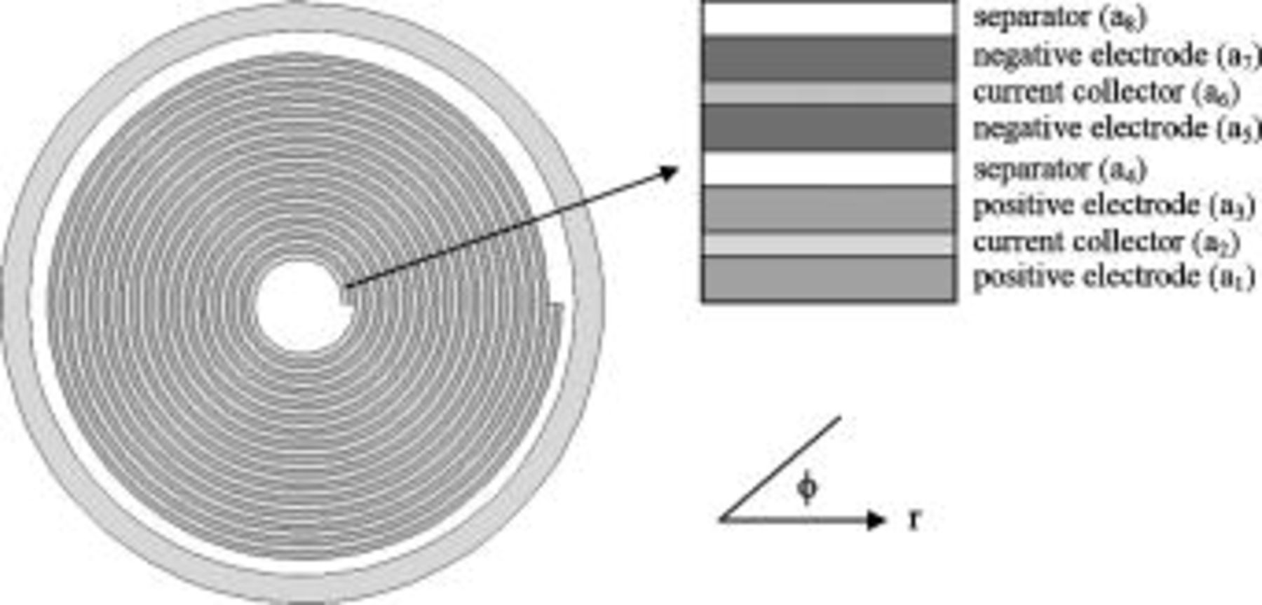
Figure 1. Cross-sectional view of a typical cylindrical battery with spirally wound design.
Development of the thermal model equations and external boundary conditions
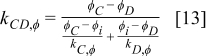
Although a battery is composed of solid materials as well as liquid electrolytes, the liquids are trapped into small pores or gaps so that their mobility is highly restricted, and therefore the contribution of convection inside a battery can be neglected. Besides, radiation effects can be neglected inside a battery because most parts of the battery are opaque materials. In this work, the adiabatic planer end surface of a battery is assumed so the axial heat flow is neglected. Hence, heat flow inside a battery is exceedingly dominated by conduction in radial and angular directions, which is given by

Note that the density, heat capacity, and thermal conductivity vary with location, because the interior of a battery is a heterogeneous system. Due to a lack of detailed information, the effects of temperature change on thermal expansion and thermal conductivity are ignored, although these factors can be included into the model with a relatively minor effort. It works well when the physical properties of these materials are not strongly dependent on temperature, or the temperature change in the system is not significant.
The heat generation rate of a battery during its operation is expressed by the following general formula


Note that most of the electrochemical reactions take place in the spiral region, and therefore the hollow core, the contact layer, and the case do not generate heat during the operation. This equation is merely for the interface of a thermal model, and the heat generation rate should be obtained from an electrochemical model. The selection of the electrochemical model depends on the objectives and the requirements of the simulation. In this work, the formula proposed by Bernardi et al.10 is adopted and written as

where  ,
,  ,
,  , and
, and  denote the current drawn from the battery, the volume of a spiral, the open-circuit potential, and the working voltage, respectively. This formula is derived based on heat generation being uniform throughout the spiral, and the effect of temperature distribution on the theoretical heat generation rate is not considered. We prefer to adopt a compact electrochemical model instead of rigorous ones to represent the heat generation rate, because the simulation results can be efficiently obtained so that we can pay full attention to thermal analysis.
The initial temperature of the battery is equal to the surrounding temperature, which is assumed constant in this work, as follows

At the boundary, both convection and radiation are considered. The boundary equations adopted in this work are analogous to those developed in our previous work11


where  is the radius of the battery,
  ,
,  , and
, and  denote the combined, convective, and radiative heat-transfer coefficient, respectively, ε means the emissivity, and σ signifies the Stefan-Boltzmann constant. The definition of
  and
and  depends on the convection type at the boundary, and three types of convective heat-transfer are discussed, as given by


where  is the height of a cylindrical battery,
  is the air velocity,
  is the distance to the leading edge,
  denotes the thermal conductivity of air,
  signifies the diameter of the battery, and
  is the local Nusselt number. The main advantage of these boundary equations is that any modification is unnecessary when the mode of convection is changed. Furthermore, by introducing the semiempirical equations instead of arbitrarily choosing a value, the heat-transfer phenomena at the boundary can be properly represented.
Internal interface and local property approximations
We need to cope with the complicated problems arising from the material interfaces in a battery. As mentioned earlier, the density, heat capacity, and thermal conductivity vary with location, and these properties cannot be represented by any continuous equation due to the existence of material interfaces. Therefore, the analytical approach is impractical to solve the governing equations, and the control-volume formulation,14 one of the prevalent numerical techniques, is adopted to analyze the thermal system. In this work, each material interface in a battery is described as an Archimedes spiral, as shown in Fig. 1, in which the locus is written as a general equation  , where
  and
and  are real numbers. The main difficulty in analyzing these interfaces is that the loci of the material interfaces are not orthogonal to any coordinate we defined. Furthermore, the contact resistance due to the imperfect contact also affects the analysis. Fortunately, this effect is insignificant and can be neglected, because most of the interfaces are filled with liquid electrolyte, and the thermal conductivity of the liquid electrolyte is comparable to that of the materials in the battery, such as the separators and the electrodes.
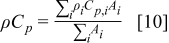
A schematic representation of the control volume is shown in Fig. 3. Note that the control volume is a fundamental block of the numerical analysis that has single and uniform physical properties. The physical properties of a control volume that does not have any interface in it are equal to the physical properties of the material on which the control volume is located. However, if a control volume contains one or more interfaces, the corresponding physical properties of the control volume should be calculated to obey the basic definition. Based on the concept that the total heat capacity of a control volume is identical before and after the transformation, the product value of density and heat capacity in a control volume can be expressed as
where  denotes the area of the material
  in a control volume. Note that it is unnecessary to calculate the individual value of the density and heat capacity, because these properties are always in product form. Based on a similar concept, the corresponding heat generation rate per unit volume can be expressed as follows
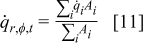
Figure 3. A schematic representation of the grid point, control volume, material interface and local thermal conductivity: (a) an orthogonal material interface and (b) a nonorthogonal material interface.
The thermal conductivity, however, cannot be transformed to the corresponding value by following a simple rule when the control volume is composed of more than one substance, because it depends on the arrangement, ratio, and individual thermal conductivity of each material. Due to the numerical formulas, the local thermal conductivity to be determined is not exactly located on a control volume but on a region between two grid points such as the gray area in Fig. 3. We started the discussion by considering the simplest case that the interfaces are orthogonal to the coordinates and are located on the boundaries of the control volumes, as shown in Fig. 3a. The interfacial thermal conductivity can be derived based on a steady one-dimensional analysis as presented by Patankar.14 For  , the following formula is derived
The expression of  can be derived in a similar way and is written as
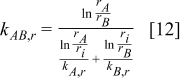
Due to the nonorthogonal material interface, as shown in Fig. 3b, the method discussed above cannot be applied and another strategy should be developed. Applying the volume fraction to estimate the local thermal conductivity may be straightforward, but it neglects the arrangement of constituent materials. Therefore, an advanced method was developed in this work to properly solve the problem. The first row of Fig. 4 shows several typical conditions for which the local thermal conductivity of a region containing material interface needs to be determined, and evidently the nonorthogonal material interface is an obstacle to obtain the solution. Therefore, the material interface is modified to several regular segments that are always parallel to the boundaries, as shown in the second row of Fig. 4, and the total area of both materials does not change after the modification. Because the local thermal conductivity of the approximated configuration can be efficiently obtained by adopting the thermal network model,15 it is applied to estimate the local thermal conductivity of the real configuration.
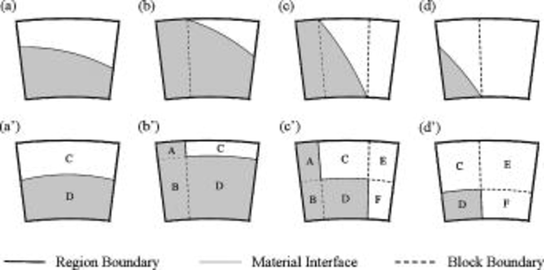
Figure 4. The actual material interface (a, b, c, d) and the first-level approximation  used to calculate the local thermal conductivity.
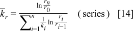
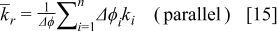
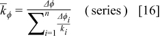
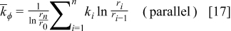
The radial thermal conductivity is calculated by connecting regions C and D in series and then combining regions AB, CD, and EF in parallel if the blocks exist. Similarly, the angular thermal conductivity is evaluated by connecting regions C and D in parallel and then combining regions AB, CD, and EF in series if the blocks exist. Note that the thermal conductivity of the combined elements can be derived based on the concept of thermal resistance15 and is expressed as follows
The approximation strategy shown above can be further extended to the high-level approximation (as shown in Fig. 5), and the accuracy of the approximated configuration as well as the calculation time increases with increase in the approximation level. This shows great flexibility because a suitable approximation level can be chosen according to the precision and the efficiency requirements. It is noteworthy that increase of the approximation level does not always increase the precision of the approximated local thermal conductivity, although it is usually true, for small levels especially.
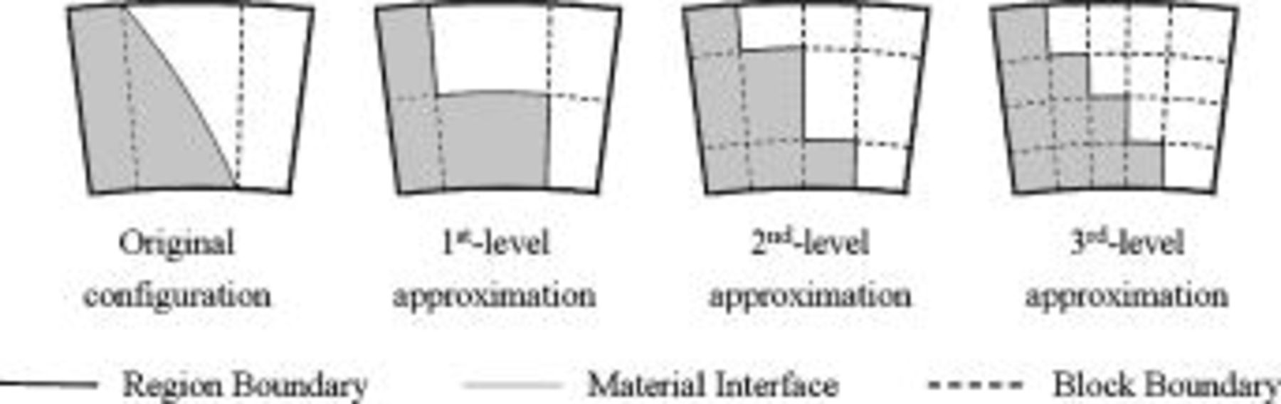
Figure 5. High-level approximation of the geometry for calculation of the local thermal conductivity.
Besides the approximation technique of the local thermal conductivity, the grid size chosen in the simulation is also an important factor. If the grid points are not dense enough, there may be several material interfaces in each control volume, and most of the local thermal conductivity should be determined by approximation. For a typical example shown in Fig. 6, when there are enough grid points, a continuous channel will exists, as shown in Fig. 6a, and distinct properties of each material can be reflected in the results. However, the continuous channel decreases or totally disappears, as shown in Fig. 6b and 6c, when the number of grid points decreases, and the simulation results do not directly come from the contribution of each material. Therefore, it is important to ensure that there are enough grid points to retain the material properties.
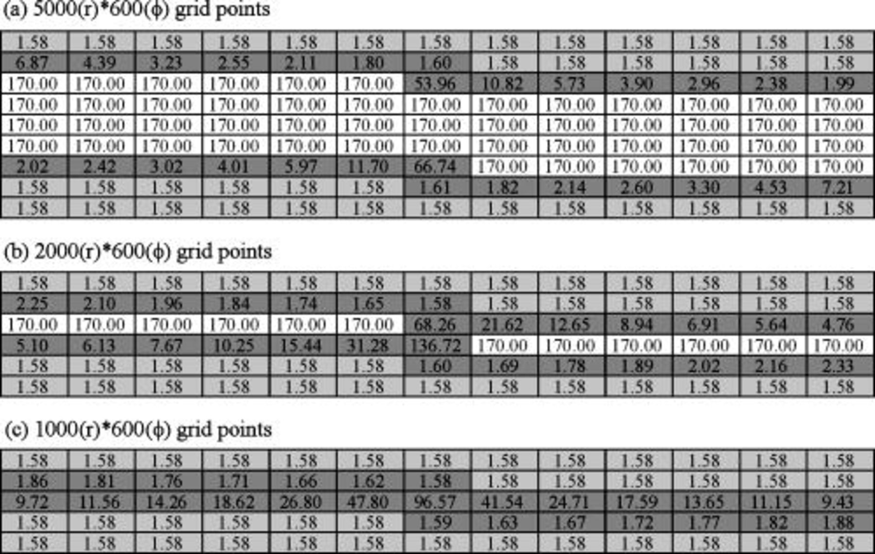
Figure 6. Partial matrices of local thermal conductivity  in various grid densities. The values are in
  . The white cell is the region of Al foil, the light gray cell denotes the electrode, and the dark gray cell indicates the interface region containing both materials.
The formulas of the detailed thermal model developed above are solved by developing a powerful program based on a multithread architecture that processes the simulation concurrently on parallel processors. The control-volume formulation with implicit alternative-direction iteration16 is the main algorithm of the solver, and each simulation proceeds until the temperature is converged to  . Although the model is designed for a spirally wound lithium battery, it can be applied to various battery systems with an analogous configuration. The model is applied to simulate the thermal behavior of a spirally wound lithium battery under typical operating conditions, including the natural convection and forced convection with a parallel flow as well as a cross flow.
Accuracy of the thermal conductivity formulations and precision of calculations
Because parts of the local thermal conductivity in the model are determined by estimation, it is necessary to examine the deviation of estimation formulas. Accuracy means deviations of thermal conductivity formulations to estimate the actual local thermal conductivity. It can be obtained by finding the upper bound and lower bound of the exact local thermal conductivity. The detailed procedure is demonstrated in the Appendix, and the results are shown in the following section.
In addition to the deviation coming from the thermal conductivity formulations, deviations are also generated from calculations—such as the tolerance of the iteration procedure, the truncation error, the round-off error, and the numerical scheme itself—although they are usually small in comparison with the previous factor. Due to errors generated from calculations, the conservation of energy may not exactly hold, and therefore it can be an index to evaluate precision of the results, which is defined as follows
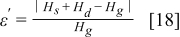
where  ,
,  , and
, and  denote heat accumulated in the system, heat dissipated from the boundary, and heat generated during the discharge, respectively. This formula is adopted to examine precision of the simulation results.
Results and Discussion
Accuracy of the thermal conductivity formulations and precision of calculations are determined according to the methods discussed above because they are the major sources that may induce departure from the actual solution. After certification, the model is adopted to analyze the thermal behavior of typical cylindrical lithium batteries. The configuration of batteries to be examined and the nomination of these batteries are listed in Table I and II, and the physical properties of the materials are summarized in Table III. Three typical operating conditions are investigated, and the detailed descriptions are listed in Table IV. Cell potential with respect to depth of discharge under 1- and 3-C discharge rate is obtained from experiments of a 10-Ah cylindrical lithium battery (no. 3), as shown in Fig. 7. Because all of the batteries listed in Table II are directly scale-up or scale-down of a 10-Ah battery (no. 3), the experimental results shown in Fig. 7 are extensively applied to all simulations due to a lack of detailed data for the other batteries.
Table III. Physical properties of each material in the battery.11
| Material | Thermal conductivity
| Density
| Heat capacity
|
|---|---|---|---|
Positive electrode 
| 1.58 | 2328.5 | 1269.21 |
| Negative electrode (carbonaceous material) | 1.04 | 1347.33 | 1437.4 |
| Current collector of positive electrode (Al alloy) | 170 | 2770 | 875 |
| Current collector of negative electrode (Cu) | 398 | 8933 | 385 |
| Separator (PP) | 0.3344 | 1008.98 | 1978.16 |
| Liquid electrolyte | 0.6 | 1129.95 | 2055.1 |
| Case (Al alloy) | 170 | 2770 | 875 |
Table IV. Discharge conditions of lithium batteries in the simulation.
| Name | Description | Boundary condition | Initial condition and heat generation |
|---|---|---|---|
| Natural convection | Natural convection (vertical cylinder) with radiation | The heat-transfer coefficient is automatically generated, and 
| Initial temperature:  Surrounding temperature: Surrounding temperature:  Heat generation rate: Eq. 3 with Heat generation rate: Eq. 3 with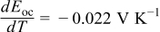 |
| Symmetrical forced convection | Symmetrical forced convection (parallel flow) with radiation |
 , ,  , and , and 
| |
| Asymmetrical forced convection | Asymmetrical forced convection (cross flow) with radiation |
 ,800, and ,800, and 
|
bFrom Ref. 17.
Figure 7. Cell potential as a function of utilization. The results are obtained from experiments of a 10-Ah cylindrical lithium battery (no. 3).
Table I. The values of  and
and  used in Eq. 7.12
| Geometry | Condition |
 
|
|

|
|---|---|---|---|---|
| Vertical plate or |
| 1.485088 | 0.0024 | 0.25 |
| Vertical cylinder |
| 0.941145 | 0.0022 | 0.35 |
Table II. Physical details of the batteries in the simulation.
| No. | Battery size (cm) | Capacity (Ah) | Dimension (cm) | Thickness of each layer 
|

| Grid points
| |||||||
|---|---|---|---|---|---|---|---|---|---|---|---|---|---|
| Diameter | Height |

|

|

|
 , , 
|

|
 , , 
|
 , , 
|

| ||||
| 1 | 0.804 | 2.36 | 0.08 | 0.04430 | 0.00230 | 0.01 | 55 | 20 | 30 | 55 | 14 | 10 |

|
| 2 | 2.412 | 7.08 | 2.16 | 0.16430 | 0.03830 | 0.03 | 55 | 20 | 30 | 55 | 14 | 30 |

|
| 3 | 4.020 | 11.80 | 10.00 | 0.28430 | 0.07430 | 0.05 | 55 | 20 | 30 | 55 | 14 | 50 |

|
| 4 | 5.628 | 16.52 | 27.44 | 0.40430 | 0.11030 | 0.07 | 55 | 20 | 30 | 55 | 14 | 70 |

|
| 5 | 7.236 | 21.24 | 58.32 | 0.52430 | 0.14630 | 0.09 | 55 | 20 | 30 | 55 | 14 | 90 |

|
| 6 | 8.844 | 25.96 | 106.48 | 0.64430 | 0.18230 | 0.11 | 55 | 20 | 30 | 55 | 14 | 110 |

|
a
 is the distance between the center and the inner radius of the spiral at
  ;
;  denotes the distance between the outer radius of the spiral and the inner radius of the case at
  ;
;  signifies the thickness of the case, and
  means the number of revolutions of the spiral. The notation of
  refers to Fig. 1.
Accuracy of the thermal conductivity formulations and precision of calculations
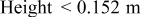
The relative deviation with respect to the whole system in various approximation levels and number of grid points due to approximation of the local thermal conductivity is depicted in Fig. 8. Because of the similar trends found in all simulations, only the results of a 10-Ah battery (no. 3) are shown in this figure. According to the results, all of the deviations of 1st-level approximation are less than 0.5%, which indicates that the thermal conductivity formulations developed in this work have high accuracy to estimate the local thermal conductivity. Increasing the approximation level or the number of grid points can further reduce the deviation, and that is quite valuable when a simulation requires very high accuracy.
Figure 8. Relative deviation of the local thermal conductivity with respect to the whole system in various approximation levels and number of grid points. The results are calculated based on a 10-Ah lithium battery (no. 3).
The model possesses great flexibility, in that accuracy of a simulation can be adjusted by changing the parameters, and more accurate results can be gained by spending more time. This is quite different from the thermal models that have been presented in the literature, because these models are physically restricted by the fundamental elements used to construct the approximated object, such as the semicircles or the concentric circles. The number of grid points used in this work is listed in Table II, and the 5th-level approximation is adopted, because the deviation shown in Fig. 8 is small enough to ensure the accuracy of approximation.
Precision of calculations, another factor that affects deviations of the simulation results, is examined based on the conservation of energy discussed above, and the maximum error of precision found in this work is  (0.00294%), which is small enough and can be neglected. Therefore, it is expected that calculations in this work possess very high precision and the simulation results are reliable.
Battery discharge under natural convection
It is sensible to investigate the thermal behavior of batteries discharged under natural convection because most batteries are designed to operate in this condition. The temperature variation of a 10-Ah battery (no. 3) under 1- and  discharge rate is depicted in Fig. 9. The average temperature15 in this figure is calculated as follows
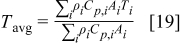
The results show that temperature rise is much more significant when a battery undergoes high-rate discharge, so thermal management is relatively important under this condition. Because a  discharge, a battery exhausting its electricity in
  , is a typical condition of high-rate discharge, this condition is chosen in this work to analyze the thermal behavior of battery discharge.
Figure 9. Variations in maximum temperature, minimum temperature and average temperature of a 10-Ah lithium battery (no. 3) under 1- and  discharge.
Temperature variation of batteries under natural convection is depicted in Fig. 10. According to the results, the maximum temperature as well as average temperature at the end of discharge increase with increasing battery size due to enhancement of the internal thermal resistance. Thermal management may not be important for the smallest battery (no. 1), because temperature rise is no more than  during discharge. However, temperature rise more than
  for the other batteries (no. 2–6) may be hazardous and should be properly handled. Due to the internal thermal resistance, the minimum temperature of a battery, which is located on the surface, approaches a constant
  when the diameter of a battery is larger than
  (no. 3), as shown in Fig. 10.
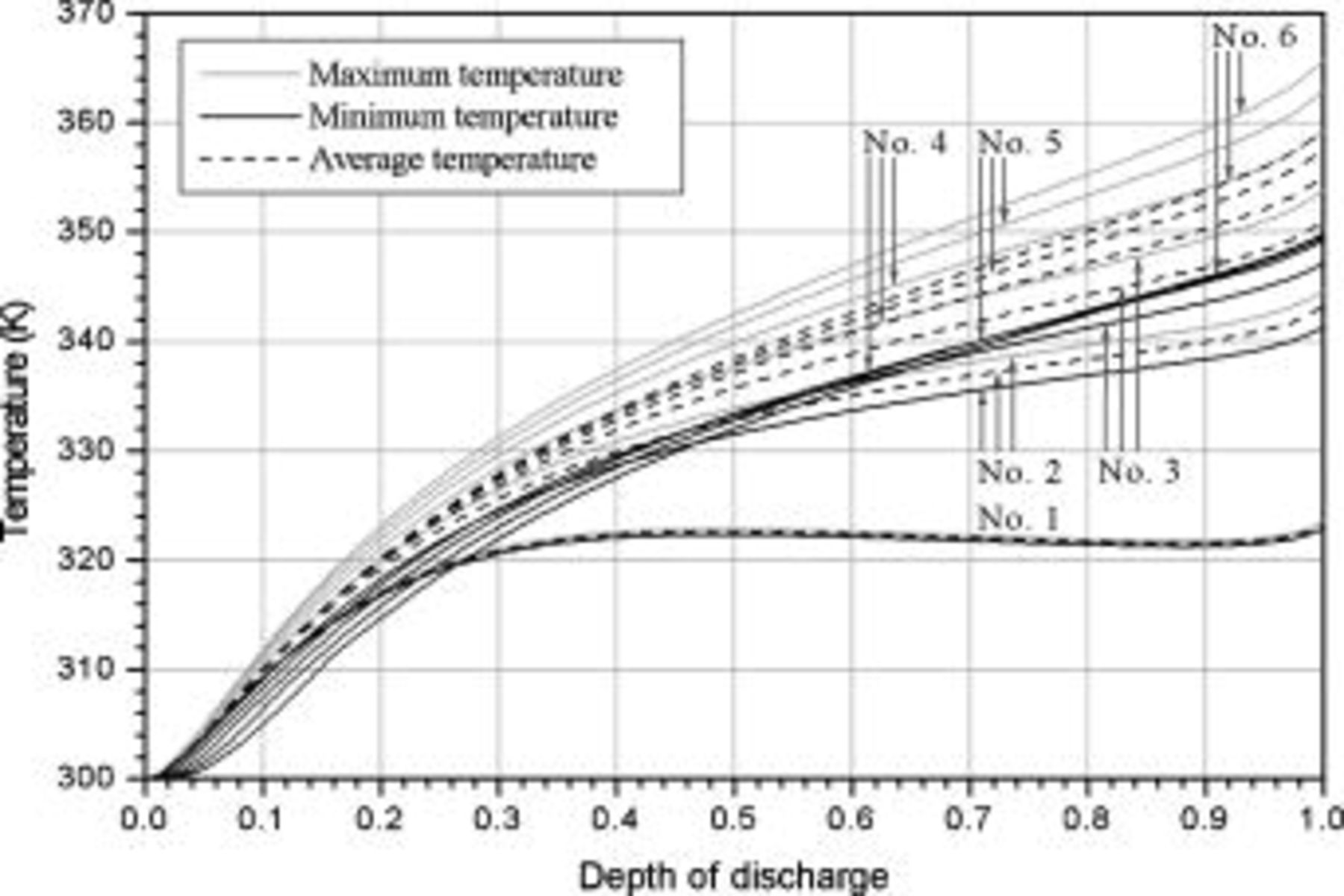
Figure 10. Variations in maximum temperature, minimum temperature, and average temperature under natural convection.
Temperature distribution at the end of discharge is shown in Fig. 11a. Although the spiral is asymmetrical, temperature at the angular direction is fairly uniform and heat is mainly transferred along the radial direction. It also shows that the maximum temperature is not located on the center but on a circular region neighboring the hollow core, because the hollow core does not generate heat during the operation. Therefore, an attempt to monitor the maximum temperature by measuring the center point of a battery does not actually obtain precise information. Because the hollow core is required by the manufacturing process and is close to the high-temperature region, installing a material with large heat capacity to absorb heat or assembling a device with excellent thermal conductivity to transport heat along the hollow core may be good strategies to manage the system temperature.
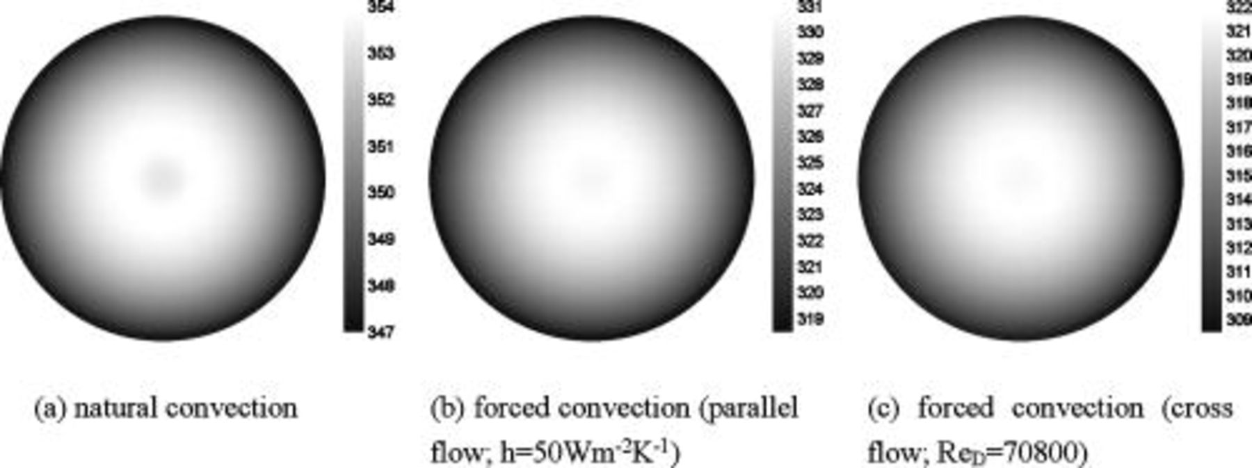
Figure 11. Temperature distribution of a 10-Ah lithium battery (no. 3) at the end of  discharge.
The radial temperature distribution is further investigated in Fig. 12. According to the results, the surface temperatures are 0.54, 3.36, 6.70, 10.02, 13.17, and  , and the center temperatures are 0.02, 0.23, 0.74, 1.49, 2.47, and
  lower than the maximum temperature for no. 1–6 at the end of discharge, respectively. Therefore, the safety of a battery cannot be determined simply by measuring its surface temperature, for large batteries especially. According to the gradient of the temperature profile, it is evident that the heat flux inside the battery is not always outward. Due to the excellent thermal conductivity of the case, the temperature gradient is quite small in comparison with the other regions. However, the junction points between the contact layer and the spiral as well as the hollow core and the spiral are not conspicuous. Accordingly, the effective thermal conductivity of the spiral is close to that of the liquid electrolytes, which means that the spiral is a poor thermal conductor.
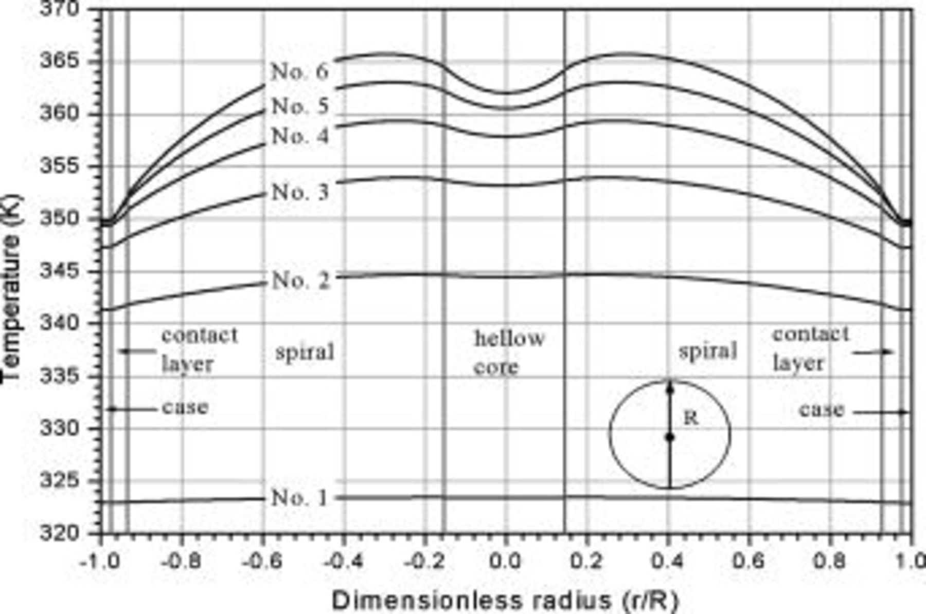
Figure 12. Radial temperature distribution  under natural convection at the end of discharge.
Due to the discontinuity of the material behavior, the radial temperature profile actually comprises a series of segments, as shown in Fig. 13, although it seems quite smooth macroscopically. The results shown in this figure are quite helpful for an engineer to improve the efficiency of the heat dissipation, because the thermal resistance of each material to the heat transfer can be easily investigated. For example, the largest temperature drop is found between a separator, which means that the separator is the critical step to the heat transfer in this region, and enhancing the thermal conductivity as well as decreasing the thickness of the separator in a unit cell is the most effective way to improve the heat dissipation.
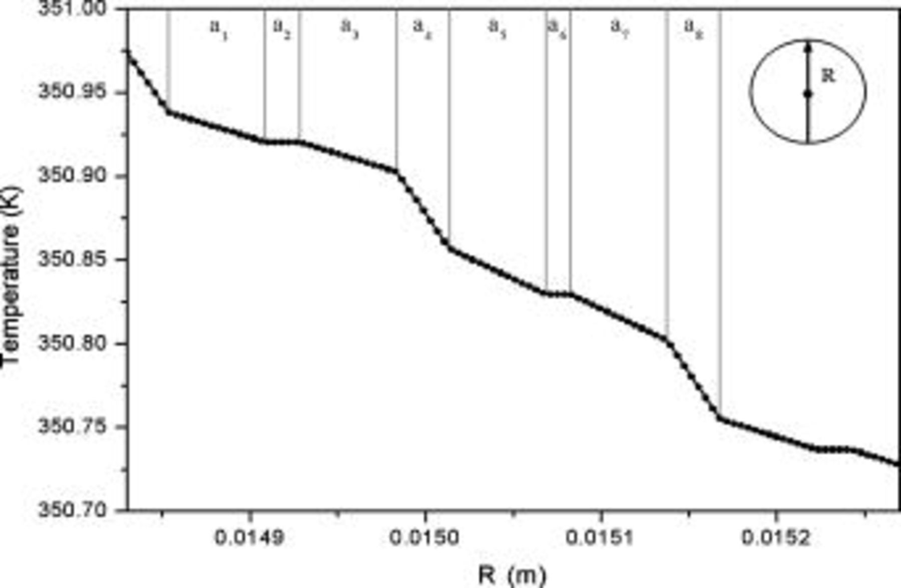
Figure 13. Radial temperature distribution  of a 10-Ah lithium battery (no. 3) under natural convection at the end of discharge. The letter near the top axis denotes the material in this region and is referred to Fig. 1.
The angular temperature profiles of a 10-Ah battery (no. 3) at the surface and at half the radius are shown in Fig. 14. Due to the asymmetrical configuration of the spiral, the temperature along the angular coordinate is not isothermal but the distribution is restricted within a narrow range. The surface temperature is highly related to the distance between the case and the spiral, and this can be revealed by comparing the results with Fig. 1. In contrast with the profile at the surface, the angular temperature distribution inside the spiral is not a smooth function due to the material interface. Note that the divergence of the angular temperature is connected to the symmetry of a spiral. For example, the surface temperature difference increases from  of the present one to
  of a battery with the same dimension, but the unit cell is 5 times thicker than the present one. Therefore, the angular temperature distribution cannot be neglected in every condition.
Figure 14. Angular temperature distribution ( and
and  ) of a 10-Ah lithium battery (no. 3) under natural convection at the end of discharge.
Because the heat-transfer coefficient under natural convection depends on the temperature difference between the surface and surrounding area, as shown in Eq. 6, 7, the value should be simultaneously determined during the simulation. Therefore, it is important to evaluate the contribution of convection as well as radiation to the heat dissipation, and the results are shown in Fig. 15. Note that the figure is depicted based on the results of no. 3, but it is close to the results of nos. 4–6 because the surface temperatures of these conditions are close to each other, as shown in Fig. 10. The results show that the contribution of natural convection is small in the beginning and is elevated during discharge. In contrast with natural convection, radiation shows weaker dependence on the surface temperature and escalates with time.
Figure 15. Heat-transfer coefficients of a 10-Ah lithium battery (no. 3) varying with time.
It is evident that supposing the heat-transfer coefficient to a constant is improper when the battery discharges under natural convection, because the coefficient in this figure varies from  and is apparently not a constant. Furthermore, neglecting radiation is also inappropriate if the surface emissivity does not approach zero, as demonstrated in Table V. The results with zero emissivity are identically equivalent to that of a model neglecting radiation, and therefore the simplified model would obtain the results as shown in the first row of the table. Apparently, neglecting radiation undervalues the maximum temperature, minimum temperature, and average temperature at the end of discharge by 3.913, 5.294, and
  , respectively, if the surface emissivity is 0.5, and the departure increases with increasing the emissivity. Therefore, a model neglecting radiation would be restricted to simulate a battery whose surface emissivity approaches zero, greatly limiting the applications of the model.
Table V. Heat dissipation of a 10-Ah lithium battery (no. 3) with various emissivities.
| Emissivity |
 at end of discharge at end of discharge |
 at end of discharge at end of discharge |
 at end of discharge at end of discharge | Maximum temperature | Minimum temperature | Average temperature | Heat dissipation (%) | Contribution of radiation (%) |
|---|---|---|---|---|---|---|---|---|
| 0.00 | 7.068 | 7.068 | 0.000 | 357.850 | 352.534 | 355.645 | 15.752 | 0.000 |
| 0.50 | 10.746 | 6.883 | 3.864 | 353.938 | 347.239 | 351.093 | 22.622 | 36.509 |
| 1.00 | 14.280 | 6.716 | 7.564 | 350.604 | 342.832 | 347.256 | 28.417 | 53.633 |


Because radiation has potential to contribute significant heat transfer at the boundary, it is possible to improve the heat dissipation by enhancing the emissivity of the surface, and the results are also depicted in Fig. 15. Increase of the emissivity slightly suppresses natural convection due to the drop of the surface temperature, as shown in Table V, but the overall heat-transfer coefficient increases due to the rise of radiation. According to the summary in Table V, the maximum temperature, minimum temperature, and average temperature decrease by 7.246, 9.702, and  , respectively, due to enhancement of emissivity from nil to unity. Furthermore, 28.417% heat generated during discharge is removed from the boundary for a battery with
  , in comparison with 15.752% for a battery with
  . Therefore, improving emissivity with proper surface treatment is an effective strategy to reduce the temperature rise.
Battery discharge under forced convection with a parallel flow
Although many strategies discussed above can be applied to enhance the heat dissipation of a battery under natural convection, it is not always efficient enough to satisfy the requirements. Thus, forced convection is generally used for a battery with high heat generation rate, because it offers much better efficiency than natural convection on heat transfer. However, forced convection directly acts on the surface and cannot guarantee that the whole battery operates with a suitable temperature range, so thermal analysis is necessary.
Temperature variation of a 10-Ah battery (no. 3) under different extents of forced convection is depicted in Fig. 16. In comparison with the results from natural convection, the maximum temperature decreases by 23.156, 30.946, and  when the heat-transfer coefficients are 50, 100, and
  , respectively. According to the summary in Table VI, most of the heat is removed via forced convection, and the contribution of radiation is as small as 6.336, 3.119, and 3.075% for
  , 100, and
  , respectively. Furthermore, 61.467, 73.751, and 78.625% of the heat generated during the discharge is removed if the heat-transfer coefficient reaches 50, 100, and
  . Temperature distribution under forced convection at the end of discharge is quite analogous to that under natural convection, except that the radial temperature gradient is much steeper due to the strong heat transfer at the boundary, and the phenomena can be investigated from Fig. 11b.
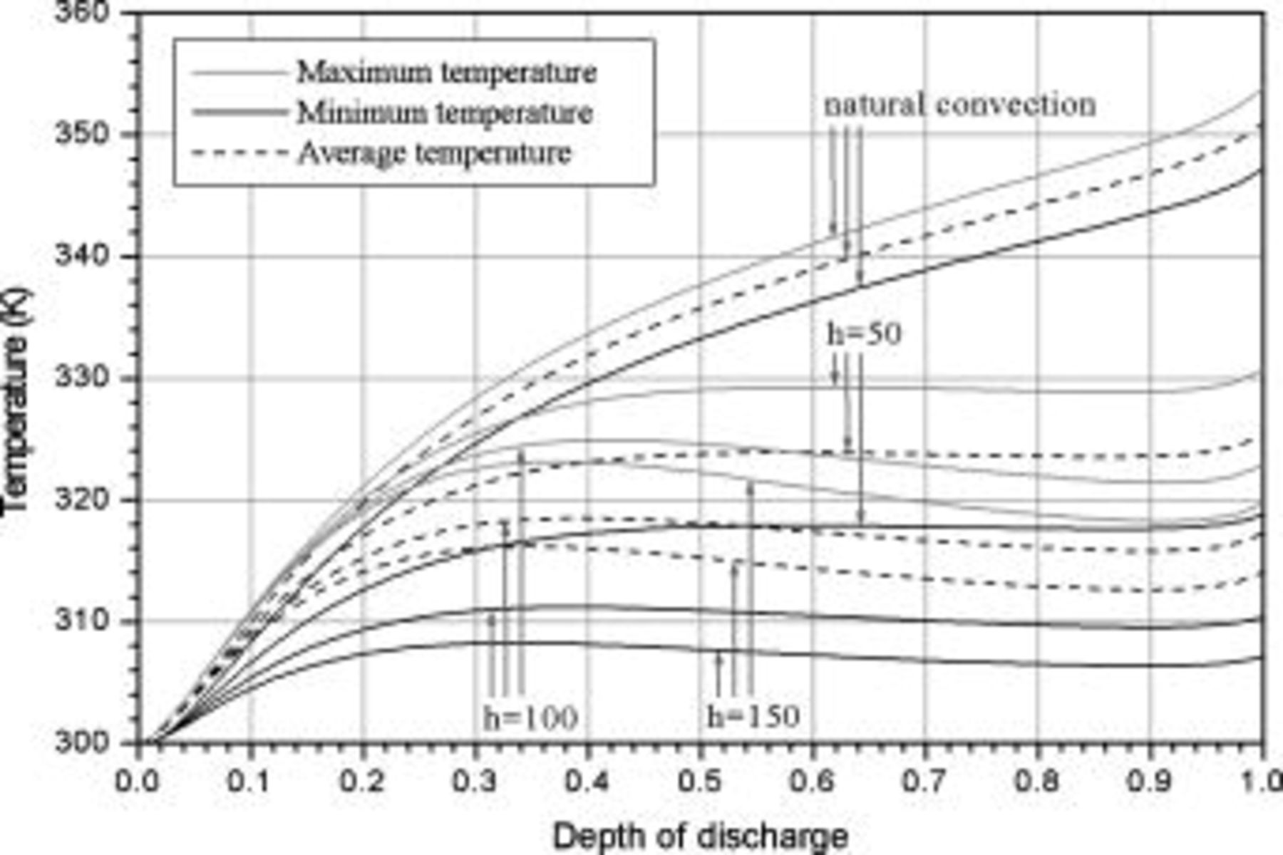
Figure 16. Variations in maximum temperature, minimum temperature, and average temperature of a 10-Ah lithium battery (no. 3) under a parallel flow. The heat-transfer coefficients are in  .
.
Table VI. Heat dissipation of lithium batteries under a parallel flow.

| Battery size | Emissivity |
 at the end of discharge at the end of discharge | Maximum temperature | Minimum temperature | Average temperature | Heat dissipation (%) | Contribution of radiation (%) |
|---|---|---|---|---|---|---|---|---|
| 50 | No. 3 | 0.50 | 3.427 | 330.782 | 318.826 | 325.425 | 61.467 | 6.336 |
| 100 | No. 1 | 0.50 | 3.105 | 303.467 | 302.769 | 303.159 | 95.600 | 3.010 |
| 100 | No. 2 | 0.50 | 3.164 | 311.361 | 306.576 | 309.241 | 86.117 | 3.074 |
| 100 | No. 3 | 0.50 | 3.225 | 322.977 | 310.421 | 317.342 | 73.751 | 3.119 |
| 100 | No. 4 | 0.50 | 3.274 | 336.095 | 313.456 | 325.878 | 60.772 | 3.145 |
| 100 | No. 5 | 0.50 | 3.303 | 347.481 | 315.231 | 333.088 | 49.834 | 3.159 |
| 100 | No. 6 | 0.50 | 3.318 | 355.995 | 316.114 | 338.693 | 41.347 | 3.165 |
| 150 | No. 3 | 0.50 | 3.174 | 319.795 | 307.166 | 314.142 | 78.625 | 3.075 |


The effectiveness of forced convection with respect to battery sizes is shown in Fig. 17. In comparison with the results from natural convection, the maximum temperature at the end of discharge decreases by 20.001, 33.352, 30.956, 23.255, 15.563, and  for no. 1–6, respectively, when the heat-transfer coefficient is
 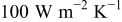 . Apparently, the effectiveness of forced convection decreases with increasing the radius of a battery due to increase of the internal thermal resistance, so applying strong forced convection may not effectively suppress the maximum temperature if a battery has as large a radius as nos. 4–6, shown in Fig. 17.
Figure 17. Variations in maximum temperature, minimum temperature, and average temperature under a parallel flow with  .
.
Clearly, forced convection is more effective than natural convection to reduce the temperature rise, but it is accompanied by a decrease of temperature uniformity, which induces the unbalanced discharge so that the battery performance decreases. For example, the temperature difference between the maximum and minimum temperature at the end of discharge is 11.942, 12.556, and  for
for  , 100, and
  , respectively. It further increases with increasing number of revolutions of a spiral as shown in Fig. 17, and an amazing value as large as
  was found for the largest battery in the simulation (no. 6). Accordingly, how to maintain the temperature uniformity to avoid the performance decline is an important subject, and that can be achieved by finding the critical step of heat transfer, as mentioned earlier.
Battery discharge under forced convection with a cross flow
In contrast with a parallel flow, the local heat-transfer coefficient under a cross flow depends on location, and heat dissipation on the surface is asymmetrical. In this work, a 10-Ah cylindrical lithium battery (no. 3) is simulated under a cross flow with air velocity to be  , which is equal to
  . The local heat-transfer coefficient is calculated according to the local Nusselt number in Fig. 2. The maximum convection heat-transfer coefficient on the surface is
  at
at  , the minimum value is
  at
at  as well as 4.964, and the average value is
  . In order to compare the effects of a cross flow and a parallel flow to the heat dissipation, an additional condition that a 10-Ah battery (no. 3) discharges under a parallel flow with
  is simulated.
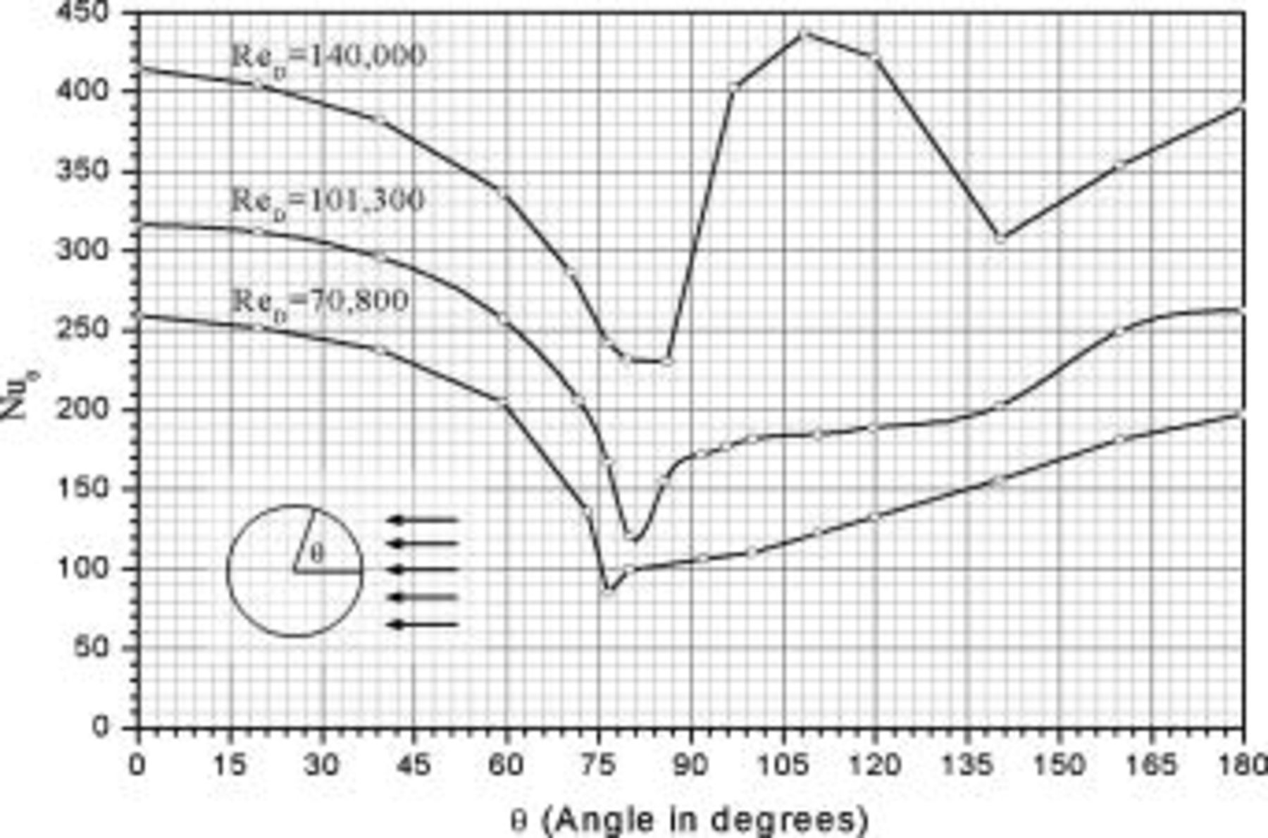
Figure 2. Variation of the local Nusselt number for airflow normal to a circular cylinder.13
Investigating the average temperature of batteries with metal cases shown in Fig. 18, the heat dissipation under a cross flow is slightly lower than that under a parallel flow if they have the same average heat-transfer coefficient. The same trend is found for batteries with plastic cases, but the difference is greater. These results are reasonable because the heat dissipation rate is not directly proportional to the heat-transfer coefficient on the surface, and the increase of the coefficient on a system under weak convection is more effective than that under strong convection because of the thermal resistance inside a battery. For a battery under a cross flow, the heat dissipation rise due to the local heat-transfer coefficient larger than the average value is not enough to compensate for the heat dissipation reduction having a coefficient lower than the average value, and therefore the overall heat dissipation under a cross flow is lower than that under a parallel flow.
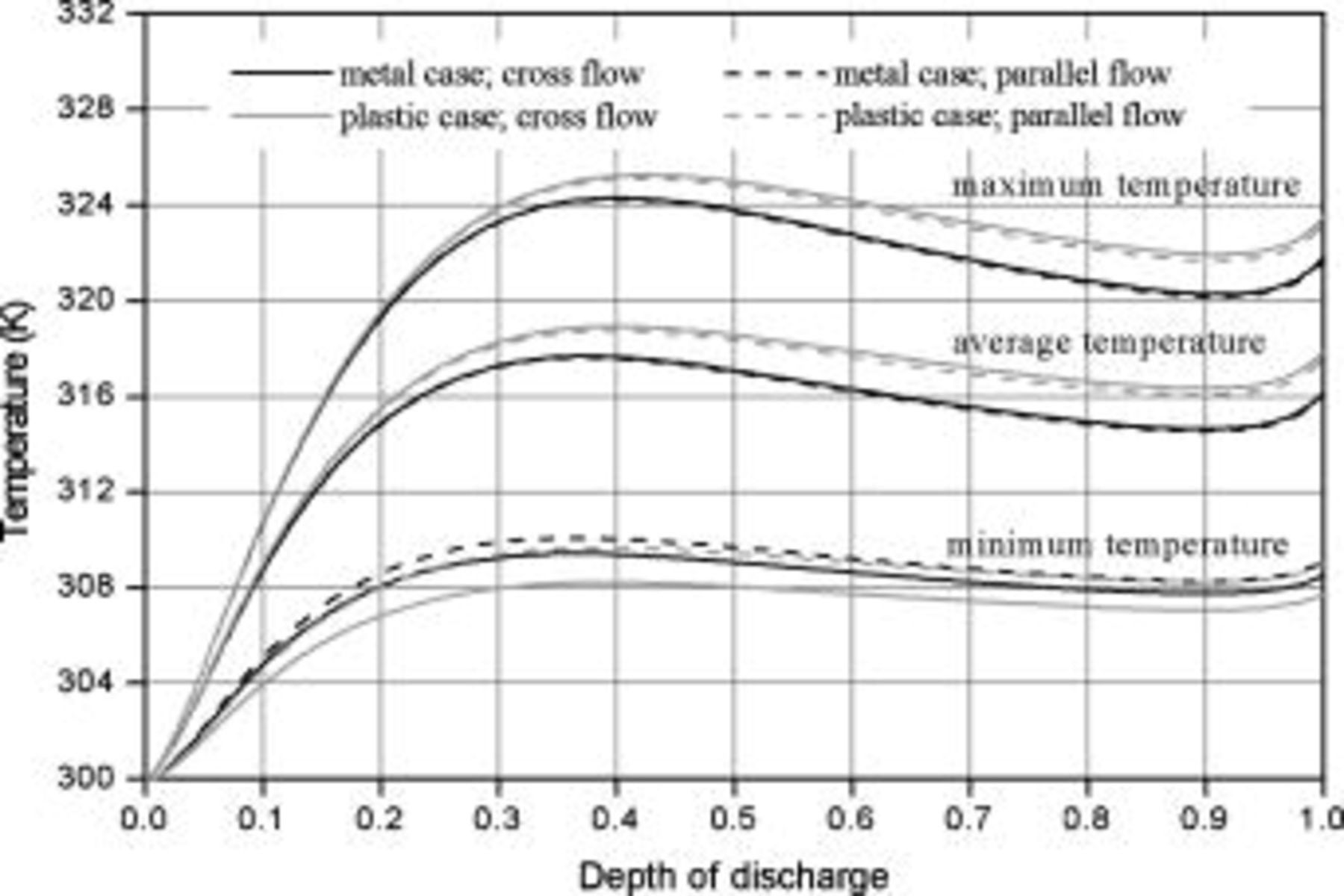
Figure 18. Variations of a 10-Ah lithium battery (no. 3) in maximum temperature, minimum temperature, and average temperature under various conditions.
The heat dissipation decline from a parallel flow to a cross flow decreases with increasing the thermal conductivity on the surface, because larger thermal conductivity exhibits more uniform temperature distribution on the surface, and this condition is closer to that of a parallel flow, as shown in Fig. 19. The heat dissipation decline of a battery with a plastic case is more serious than that of a battery with a metal case, as shown by the average temperature in Fig. 18, so a battery case with high thermal conductivity is helpful to maintain the heat dissipation performance under various types of air flows. Although the surface heat-transfer rate is asymmetrical for a battery under a cross flow, it mainly affects the regions near the surface and not the whole battery, as shown in Fig. 11c. Therefore, the temperature distribution inside a battery is not strongly altered and is analogous to that under a parallel flow. According to the results, the decline is generally acceptable for a practical application, as summarized in Table VII, and the thermal behavior of a battery under a cross flow can be roughly examined under a corresponding parallel flow with the average convection heat-transfer coefficient to avoid the complexity.
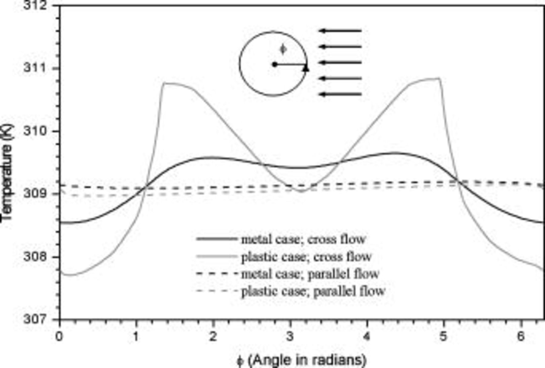
Figure 19. Angular temperature distribution  of a 10-Ah lithium battery (no. 3) under forced convection at the end of discharge.
Table VII. Heat dissipation of a 10-Ah lithium battery (no. 3) under a cross flow 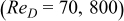 and a corresponding parallel flow.
| Flow type | Case | Emissivity |
 at the end of discharge at the end of discharge | Maximum temperature | Minimum temperature | Average temperature | Heat dissipation (%) | Contribution of radiation (%) |
|---|---|---|---|---|---|---|---|---|
| Cross | Metal | 0.50 | 3.195 | 321.794 | 308.543 | 316.138 | 75.583 | 2.493 |
| Cross | Plastic | 0.50 | 3.182 | 323.467 | 307.712 | 317.865 | 73.195 | 2.262 |
| Parallel | Metal | 0.50 | 3.204 | 321.703 | 309.093 | 316.047 | 75.722 | 2.684 |
| Parallel | Plastic | 0.50 | 3.202 | 323.200 | 308.976 | 317.594 | 73.603 | 2.681 |
e
 ,
,  , and
, and  in
in  , and temperatures in K. f
 for a parallel flow.
Conclusion
A detailed two-dimensional thermal model is developed to establish a standard for the simulation of spirally wound cells. It properly represents the configuration of the hollow core, the spiral, the contact layer, and the case in a battery to avoid deviations due to improper approximation of the spiral geometry. Furthermore, the flexible boundary equations adopted in the model make possible the simulation of various boundary conditions, such as the natural convection, the parallel flow, and the cross flow. The complicated problem arising from the local thermal conductivity across the material interface is solved by developing an approximation formula to estimate the corresponding property, and the accuracy of approximation is further examined by determining the maximum error of approximation.
According to the examination, the relative error in accuracy due to approximation of the local thermal conductivity is less than 0.22% for a 10-Ah lithium battery. The error of the simulation results due to calculations that cannot be avoided for a numerical technique is further evaluated by the conservation of energy, and the results show that the error in all of the simulations is less than  (0.00294%). Accordingly, simulation results of very high precision can be certified. Furthermore, the model possesses great flexibility in that the precision of the results can be adjusted by changing the approximation level and the number of grid points so that more accurate results can be obtained by spending more time on calculation.
Inspecting the results from the simulation shows that the maximum temperature of a battery is in a circular region near the hollow core but not exactly located in the center, because the hollow core does not generate heat, which is passively heated by the spiral. Therefore, the value measured at the center of a battery is not the maximum temperature of the system. Due to the large thermal resistance inside a battery, the difference between the maximum temperature and the surface temperature is significant, and this increases with more revolutions of the spiral, so the surface temperature is not sufficient as a security index of a battery. The results also show that the heat dissipation of a battery can be significantly improved by enhancing the surface emissivity, and therefore it is an effective strategy to the thermal management.
According to the simulation results of forced convection with a parallel flow, the effectiveness of forced convection decreases with increasing the radius of a battery, so applying strong forced convection is insufficient to suppress the maximum temperature if a battery has large radius. Furthermore, an additional problem arises due to the decrease of the temperature uniformity, and it will induce a performance decline because of the unbalanced discharge. This problem can be minimized by investigating the radial temperature profile inside a battery microscopically. Then the critical steps of the heat transfer can be found, and the temperature uniformity can be effectively improved by modifying those materials.
Due to the asymmetrical heat transfer, the surface temperature of a battery under a cross flow is affected by the distribution of the local heat-transfer coefficient, but the effects of a cross flow do not strongly influence the thermal behavior inside a battery, and the temperature distribution in most of the regions far from the surface is quite analogous to that of a parallel flow. According to the analysis, a material with high thermal conductivity is suggested for use as the battery case because it maintains a heat dissipation rate similar to that of a battery under various flow types. Furthermore, the thermal behavior of a battery under a cross flow can be roughly examined under a corresponding parallel flow with the average convection heat-transfer coefficient to avoid the complexity.
Acknowledgments
This work has been supported by the Materials Research Laboratories of Industrial Technology Research Institute. The authors especially thank Dr. M. H. Yang and J. C. Fang for helpful assistance.
National Tsing Hua University assisted in meeting the publication costs of this article.
List of Symbols

| positive electrode (the 1st layer of a unit cell) |

| current collector (the 2nd layer of a unit cell) |

| positive electrode (the 3rd layer of a unit cell) |

| separator (the 4th layer of a unit cell) |

| negative electrode (the 5th layer of a unit cell) |

| current collector (the 6th layer of a unit cell) |

| negative electrode (the 7th layer of a unit cell) |

| separator (the 8th layer of a unit cell) |

| area of a specific element  , , 
|

| heat capacity, 
|

| heat capacity of a specific element  , , 
|

| diameter of a battery, m |

| working voltage, V |

| open-circuit potential, V |

| coefficient of Eq. 6, 
|

| coefficient of Eq. 7, 
|

| convective heat-transfer coefficient, 
|

| combined heat-transfer coefficient, 
|

| radiative heat-transfer coefficient, 
|

| heat dissipated from the boundary, J |

| heat generated during the discharge, J |

| heat accumulated in the system, J |

| total current, A |

| angular thermal conductivity, 
|

| thermal conductivity of the air, 
|

| local radial thermal conductivity between element A and B, 
|

| local angular thermal conductivity between element C and D, 
|

| radius thermal conductivity, 
|

| coefficient of Eq. 6 |

| local Nusselt number |

| characteristic length, m |

| heat generation rate per unit volume, 
|

| heat generation rate per unit volume of a specific element  , , 
|

| average heat generation rate per unit volume of a specific element, 
|

| radius, m |

| Reynolds number |

| time, s |

| temperature, K |

| average temperature of the system, K |

| temperature of a specific point on the surface, K |

| ambient temperature, K |
| V | velocity of airflow 
|

| area of a specific control volume i 
|

| total volume of the spiral 
|
| x | distance to the leading edge (m) |
Greek
| ε | emissivity; exact relative deviation |

| maximum relative deviation |
| ε' | relative deviation due to the calculation |
| θ | angle in degrees |
| ρ | density, 
|

| density of a specific element i, 
|
| σ | Stefan–Boltzmann constant, 
|
| ϕ | angle in radians |
:
Appendix
Procedure to Evaluate Accuracy of Thermal Conductivity Formulations
The procedure to examine the error in accuracy due to approximation of the local thermal conductivity is explained by a typical example shown in Fig. A-1. The outer boundary depicts the territory of a local thermal conductivity that should be determined, and a nonorthogonal interface separating two different materials passes through this region. In order to evaluate the bounds of the exact value, the territory is divided by numerous regular blocks that are used to approximate the configuration of the original object. If a block is located on a single material, the properties of the block are the same as those of the material. If a block contains interfaces, the properties of the block can be equal to those of the material above the interface, as shown in Fig. A-1a, or the same as those of the material below the interface, as shown in Fig. A-1c. Apparently, both the cases roughly depict the configuration of the sector, and the exact configuration is between the two cases. The accuracy can be further enhanced if more blocks are used, as shown in Fig. A-1b and A-1d, and it is expected that both these cases will approach the exact configuration as the block size approaches zero.
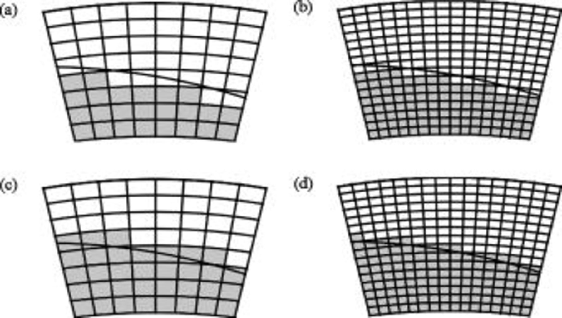
Figure 20. Procedure to evaluate the precision of the approximation. The outer boundary signifies the territory in which the approximated local thermal conductivity is evaluated, and the small blocks inside the boundary indicate the control volumes that are used to find the upper bound and the lower bound of the exact local thermal conductivity.
Thermal analysis of the approximated configuration can be properly simulated by adopting the grid system shown in Fig. 3a without approximation, because the blocks act as the control volume, the boundaries of the blocks are orthogonal to the coordinates, and the material interfaces are always on the boundaries. Each of the approximated structures is simulated on a steady-state condition with two isothermal boundaries at the concerned direction and two adiabatic boundaries at the other direction. The average thermal conductivity in the concerned direction can be obtained by monitoring the total heat flow rate at the boundaries. Note that the two isothermal boundaries are in different temperature, but the choice of the temperature value does not affect the result of the average thermal conductivity.
A typical example that analyzes the radial thermal conductivity of a sector comprising both copper above the interface and negative electrode below the interface is shown in Fig. A-2. The upper bound is the result from the approximated configuration such as Fig. A-1a and A-1b, and the lower bound comes from the results such as Fig. A-1c and A-1d. Clearly, the exact average thermal conductivity ranges from the lower bound to the upper bound, and this information can be used to calculate the maximum relative error of the approximated thermal conductivity. Although increasing the number of blocks can obtain a more precise as well as a smaller relative error, we always chose 160 blocks for each direction due to the computation time. It is noteworthy that the exact relative error may be much smaller than the value we calculated, because the maximum relative error is evaluated based on the bound with larger distance to the approximated value.
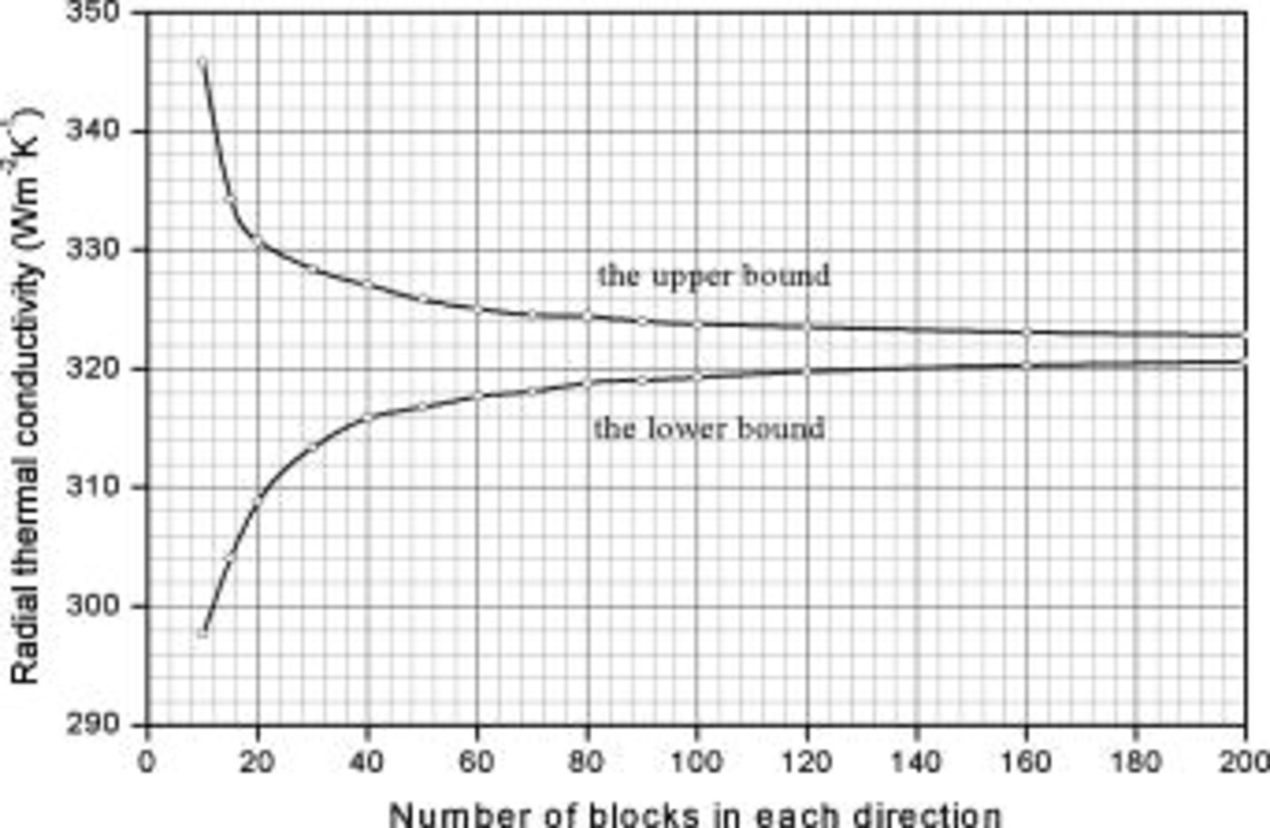
Figure 21. Simulation results of the approximated structure with different number of blocks. The original sector is composed of copper ( ; above the interface) and the negative electrode (
 ; below the interface). The dimension of the sector is
  (
( in SI unit). The interface is expressed as
  .
.
After analyzing the maximum deviation of each control volume containing interfaces, the maximum relative error of the thermal conductivity with respect to the whole system can be evaluated as follows
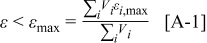
where ε,  , and
, and  denote the exact relative error, the maximum relative error, and the area of a specific control volume, respectively. The value of
  is nil for a control volume without interface, but otherwise the value should be evaluated by the procedure discussed above. Note that this analysis is also an approach to estimate the local thermal conductivity, and accuracy of this method is even better than that of the approximation formulas derived earlier. However, the tremendous calculations required make this approach impractical for real-time simulation, which means that the thermal conductivity as well as the other physical properties change with time and should be dynamically determined. Hence, it is only applied to justify the approximation.