
Abstract
Many processes contribute to the overall impedance of an electrochemical cell, and these may be difficult to separate in the impedance spectrum. Here, we present an investigation of a solid oxide fuel cell based on differences in impedance spectra due to a change of operating parameters and present the result as the derivative of the impedance with respect to  . The method is used to separate the anode and cathode contributions and to identify various types of processes.
Export citation and abstract BibTeX RIS
Mathematical techniques have been proposed to assist in the problem of identifying electrochemical processes in impedance spectra. Schichlein et al.1 have presented a technique using Fourier transformation of experimental impedance spectra in order to determine the distribution function in the time domain. In a series of papers Vladikova, Stoynov, and co-workers2, 3 use the derivative of the impedance with respect to frequency as a working variable. They resolve the impedance spectra into a series resistance, a polarization resistance, and a polarization capacitance, all of which are frequency dependent. A somewhat similar approach was later presented by Darowicki.4
These methods extract information about the contributing processes from a single impedance spectrum. In contrast, we use several spectra to isolate the process contributions prior to the data treatment. This enables us to identify and study the contributing processes separately.
The cathode and anode electrode arcs typically overlap in impedance spectra recorded on solid oxide fuel cells (SOFCs). To overcome this problem, impedance spectroscopy has been applied to both symmetrical cells (cells with two identical electrodes on either side of the electrolyte) and to electrodes in a three-electrode setup.5–10 Both experimental arrangements suffer the drawback of differing substantially from commercial cells due to the differences in manufacturing. Not only the interpretation of the spectra but also the performance and stability of the electrodes differ from that of anode-supported SOFCs with a thin  electrolyte. In this work, an SOFC is investigated and, using the presented method, six electrode processes are resolved in the impedance spectra.
The method is based on the change that occurs in an impedance spectrum when an optional operation parameter such as partial pressure of a reactant, temperature, etc., is changed. An impedance spectrum is recorded just before such a change and another spectrum just after the change. The real part of the spectra is differentiated with respect to  , where
  is the frequency. The difference in this quantity,
  , between the two spectra is named
  and is plotted vs
  . The resulting spectrum enables detection of processes affected by the altered operation parameter. The difference in the imaginary part of the two impedance spectra (named
  ) contains almost the same information. However, plotting
  vs
vs  does not provide the same resolution in the frequency domain. This is discussed theoretically in the appendix and confirmed by the presented experiments. In addition, the
  spectrum may provide detailed information about the nature of the involved processes.
Experimental
The tested cell is an anode-supported thin electrolyte SOFC.11, 12 It has a porous support layer of Ni and yttria-stabilized zirconia (YSZ) with a thickness of  . The hydrogen/steam electrode (thickness
  ) is porous and made of Ni and YSZ. The dense YSZ electrolyte has a thickness of
  . The
. The  electrode is porous and
  thick. It is made of strontium-doped lanthanum manganite (LSM) and YSZ.
The cells were tested at ambient pressure in alumina housing between two gas-distributor plates made of Ni and LSM. Ni and Au foils contacting the Ni and LSM gas distribution layers, respectively, were used for current collection. Further details on the setup are given elsewhere.13
The cell was tested at  at open-circuit voltage (OCV). The feed gas to the LSM/YSZ electrode was
  mixtures at a rate of
  ranging from pure
  to
to 
 . The feed gas to the Ni/YSZ electrode was
  mixtures at a rate of
  ranging from
 and
and 
 .
.
In one experiment the feed gas to the Ni/YSZ was different; the electrode was fed with a  (or
(or  ) mixture at a rate of
  . The
. The  (or
(or  ) concentration was
  . In this experiment the isotope was exchanged but the humidity and flow rate was kept constant.
A Solartron 1260 was used for the impedance measurements. All spectra were recorded with six measurement points per decade.
Theory
The performance of electrochemical cells depends on a sequence of processes, such as mass transfer of reactants/products, charge-transfer reactions, electronic and ionic conduction, etc. The overall impedance can be represented as a series of impedance elements describing the individual processes, i.e.
The individual  elements may be parallel circuits themselves, consisting of several processes. However, parallel connections of impedance elements such as
  circuits,
  circuits, and Gerischer elements are redundant and no separation into individual elements by means of electrochemical measurement techniques may be possible. Even when
  is known in a large frequency range, it may prove difficult if not impossible to determine the individual
  elements.
Now suppose an operation parameter, Ψ (flow rate, gas composition, temperature, etc.), is slightly changed from condition A to condition B. As a result, a number of impedance elements,  , are modified and a number,
  , stays constant. Hence, for this small change in Ψ, say
  , the change in
  can be written as

where  are omitted for simplicity. We now define
The change in  can then be written as

Hence, with a careful choice of Ψ it is possible to extract a signal from one or a few elements present in the sum of elements in Eq. 1. This makes it possible to selectively detect elements contributing in the impedance spectrum where the contribution may be hidden in overlapping contributions from other elements.
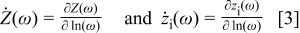
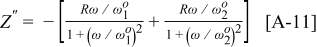
As an example, let us consider an  circuit. For further analysis, see the Appendix. Figure 1 shows the impedance arc of an
  circuit in conditions A and B. The values of the circuit elements for each impedance arc are shown in the figure. Values of ω are given for the closed symbols.
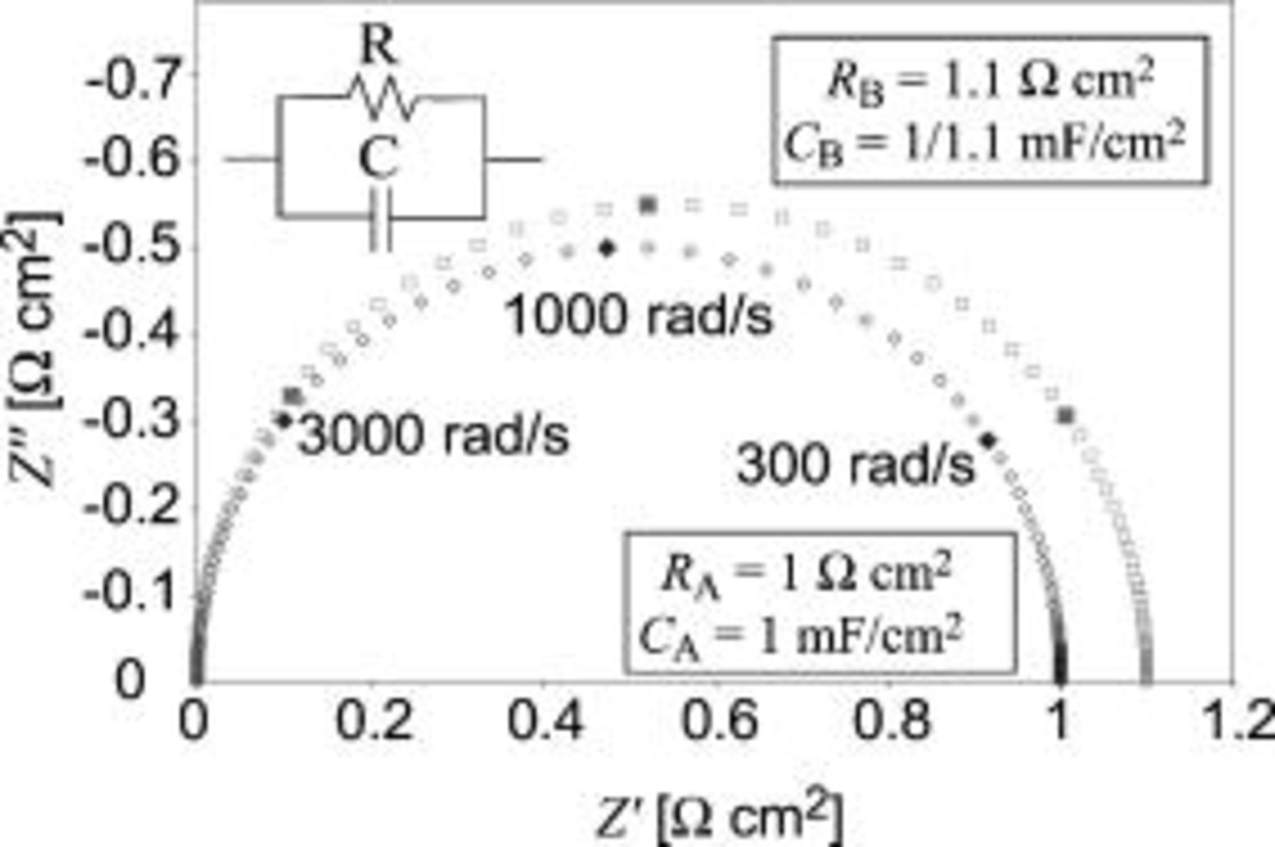
Figure 1. The impedance arcs of an  circuit in condition A and B. Element values are given in the figure. Angular frequencies are presented for the closed symbols.
Because  is only known for a discrete set of frequencies
  , for the
  frequency between 2 and
  , the real part of Eq. 4 can be rewritten as
where  is the real part of the spectrum in Fig. 1 in condition A at the frequency ω and
  is the real part of the other spectrum at ω.
  is plotted vs log frequency in Fig. 2 and labeled "
 inc.,
inc.,  dec." Such a plot of
  vs log frequency is referred to as a
  spectrum. In Fig. 2, some other
  spectra are shown for various increases (all 10% increase) and decreases (all 9% decrease) of
  and
and  .
.
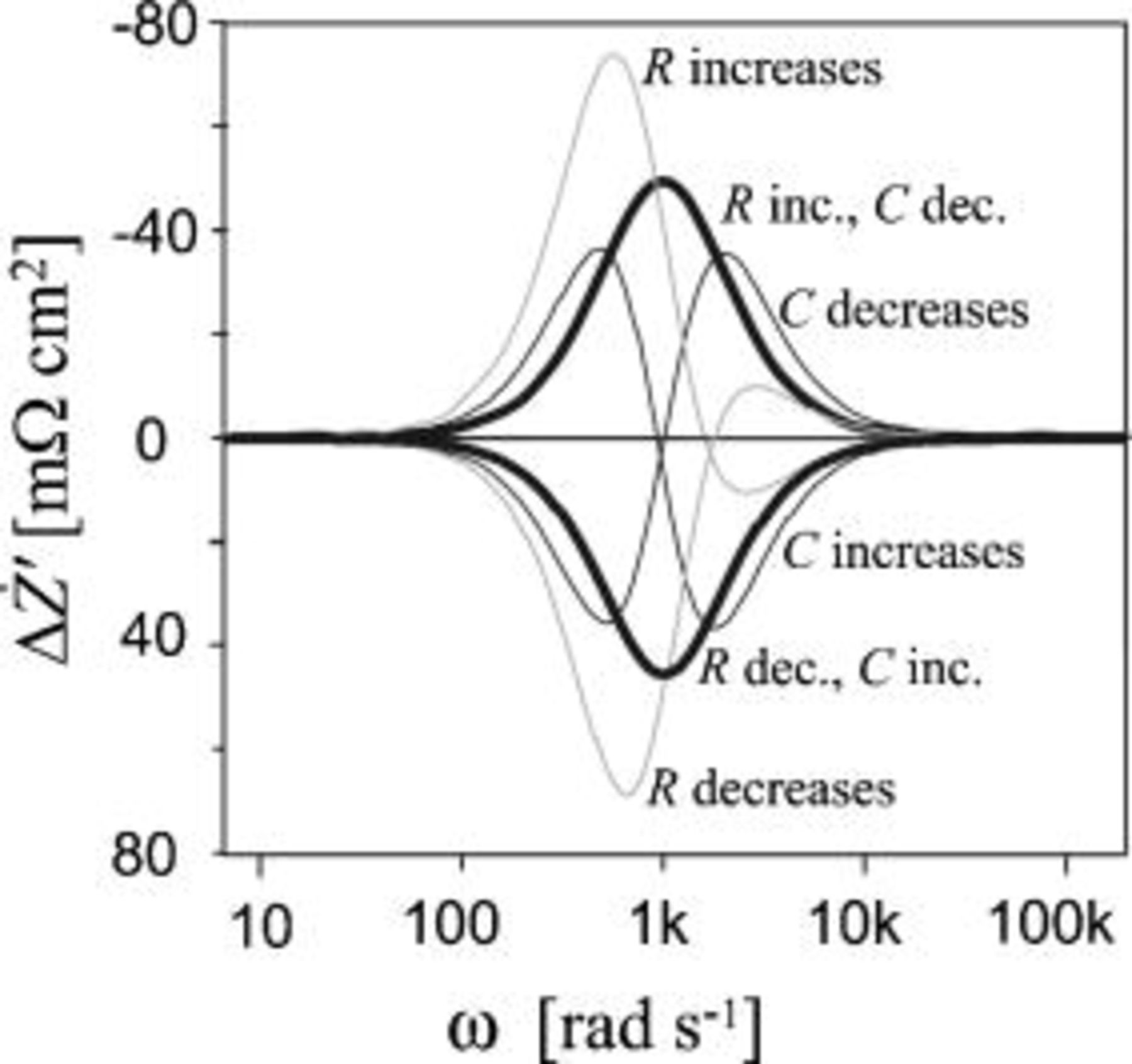
Figure 2. Theoretical  spectra for various changes in an
  circuit. Initial values are
  and
and  . All increases are 10% and all decreases are 9%.
Two main types of  spectra are defined: (i) Time invariant: The size of the impedance arc is changed, but the characteristic frequency
  is constant. The
  spectra "
 inc.,
inc.,  dec." and "
 dec.,
dec.,  inc." in Fig. 2 are time invariant because
  is constant. (ii) Time variant:
  is changed. The size of the arc may be constant or change. Two subtypes are defined. "Capacitive" is change in capacitance
  with a constant
  . The
. The  spectra "
 decreases" and "
 increases" in Fig. 2 are capacitive. "Resistive" is change in the resistance
  with a constant
  . The
. The  spectra "
 increases" and "
 decreases" in Fig. 2 are resistive.
A number of simple models of physical changes result in a time-invariant  spectrum. For instance, a change in the exchange volume in a continuous stirred tank reactor (CSTR) model of conversion impedance8 would result in a time-invariant
  spectrum. Likewise, one could think of processes related to the triple-phase boundary (TPB) (such as adsorption or desorption) that would produce a time-invariant
  spectrum if the length of the active triple phase boundary is changed (because the double-layer capacitance is inverse proportional to the TPB length, whereas the resistance associated with the process is proportional to the TPB length).
In Fig. 2, the time-invariant  spectrum only attains positive values or negative values, whereas both the capacitive and resistive
  spectra attain both negative and positive values. In the Appendix it is shown that this also applies to
  circuits and to Gerischer elements. This makes it possible to distinguish the time-invariant
  spectrum from the capacitive or resistive
  spectrum. Note that for a time-invariant
  spectrum of an
  circuit,
  has its peak frequency (i.e., local maximum or minimum) at
  .
.
Results
Figure 3 shows impedance spectra recorded on an SOFC. The upper figure shows spectra recorded with  diluted with 0, 20, 50, or
 supplied to the LSM/YSZ electrode at a rate of
  . The Ni/YSZ electrode was fed with
  containing
 at a rate of
  . The lower figure shows spectra recorded with pure
  (
(
 ) supplied at a rate of
  to the LSM/YSZ electrode and with
  containing 5, 20, or
 supplied at a rate of
  to the Ni/YSZ electrode.
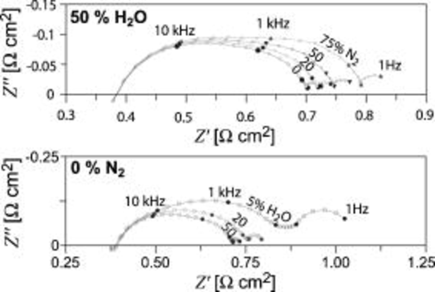
Figure 3. (Top) Impedance spectra recorded with  diluted in 0, 20, 50, or
 fed to the LSM/YSZ electrode and
  containing
 to the Ni/YSZ electrode. (Bottom) Impedance spectra recorded with
  containing 5, 20, or
 fed to the Ni/SZ electrode and pure
  to the LSM/YSZ electrode.
At first glance, the spectra in Fig. 3 show three separable arcs. In order to obtain more detailed information about the number of  that contribute to the SOFC spectra and to which of the electrodes the
  belong, the spectra in Fig. 3 were used to form
  spectra.
Referring to the upper part of Fig. 3, an impedance spectrum was recorded with pure  to the LSM/YSZ electrode. Then, the gas to the LSM/YSZ electrode was changed to
  diluted with
  and another spectrum was recorded. Finally, the gas was reverted to pure
  and a third spectrum was recorded. A
  spectrum was made using the first and second impedance spectrum as described in the previous section. Another
  spectrum was made using the second and third spectrum. By subtracting the second
  spectrum from the first and dividing by two, an average
  spectrum was made.
The average  spectrum is better than the single-shift
  spectrum in the sense that the signal-to-noise ratio is increased by a factor of 2. Furthermore, time-dependent passivation or activation of the electrodes that is unaffected by the gas change is suppressed by an order of magnitude.
In order to assure that a drift or extended relaxation due to the gas change does not influence the impedance spectra, it should be checked that the spectra obey the Kramers–Kronig relations. Because electrical circuit models satisfy the Kramers–Kronig relations, a system can be judged to be stationary if a satisfactory fit to an equivalent circuit model can be obtained.14, 15
All the impedance spectra are tested by modeling the spectra with an equivalent circuit of the Voigt type,  .
.  is an inductance in series with
  , an ohmic resistance. The brackets indicate that
  is a parallel circuit consisting of a resistance and a constant phase element.
  is a finite-length Warburg element with a transmissive boundary condition.16 The error between fit and measurement relative to
  was less than 1% for both the real and imaginary part in all spectra at all frequencies. Hence, drift or extended relaxation is known to be limited.
The noise in the resulting average  spectrum was further reduced by using a moving average of three points, plotting each point,
  , as an average of the values obtained at
  , and
, and  . The result is shown in Fig. 4. A noise-reduced (or moving average of three points)
  spectrum from
 to
to 
 was made to measure the uncertainty or background noise of the measurement technique and is plotted as the bold black line.
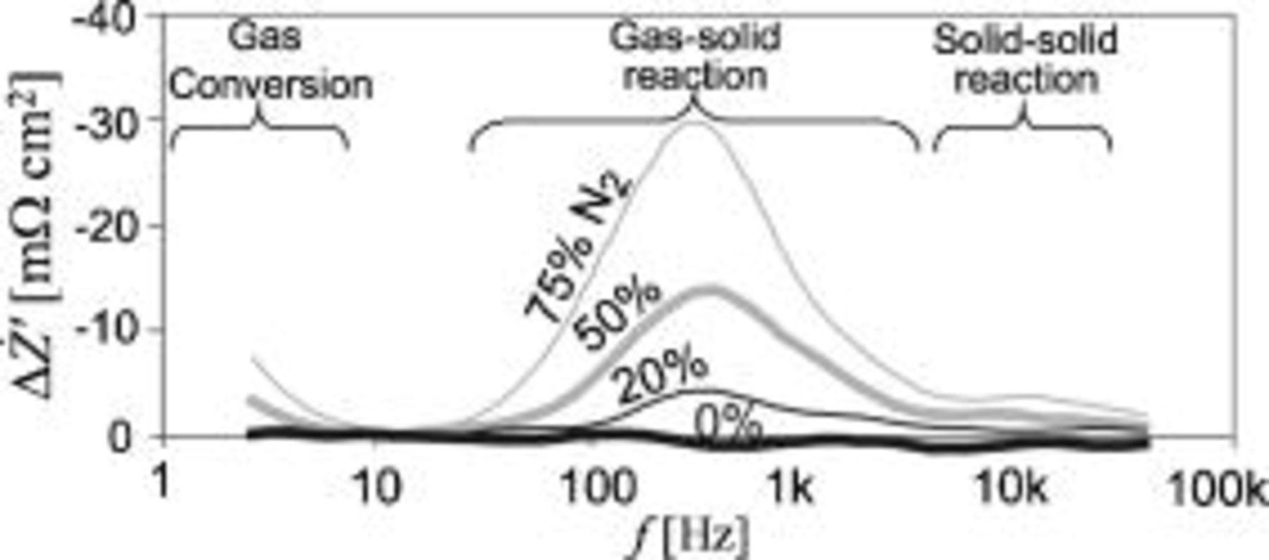
Figure 4.
 spectra recorded on an SOFC with a gas shift to the LSM/YSZ electrode from pure
  to
to  diluted in 0, 20, 50, or
 . The bold line (0%) is a background noise measurement. All spectra are recorded with
  containing
 to the Ni/YSZ electrode.
The number of measurement points used in this work is six points per frequency decade. The synthetic  spectra (shown in the Appendix) indicate that the peaks, which we probably would find, are stretched over a frequency decade or even more. For this reason, it is unlikely to find any additional features in the
  spectra by increasing the number of frequency points per decade.
If the number of points were increased, the time used to produce the impedance spectra would increase. This may increase possible errors due to drift, electrode relaxation, or unstable measurement conditions. Increasing the number of ac cycles at each measurement point also decreases the noise provided that no changes over time take place. Thus, the optimal number of points per frequency decade as well as the optimal number of ac cycles per point has to be assessed in each case.
The  spectra in Fig. 4 reveal three separable peaks, indicating that at least three different types of processes occur at the LSM/YSZ electrode and contribute to the impedance spectra. The summit frequency,
  , of the LSM/YSZ electrode arcs in pure
  can be approximated by drawing a straight line through the peaks of the
  spectrum to the
  axis. The frequency at the intercept with the
  axis is the approximate summit frequency for the LSM/YSZ electrode arcs in pure
  . These frequencies are
  . The processes behind the three observed peaks are elaborated on in the next section.
Referring to the lower part of Fig. 3, an impedance spectrum was recorded with  containing
 to the Ni/YSZ electrode. The steam concentration was subsequently changed to 5 or
 and another impedance spectrum was recorded. Finally, the steam concentration was reverted back to
 and a third spectrum was recorded. The spectra were used to produce average noise-reduced
  spectra like the ones shown in Fig. 4. The result is shown in Fig. 5. A noise-reduced
  spectrum from
 to
to 
 was made to determine the background noise of the measurement technique and is plotted as the bold black line.
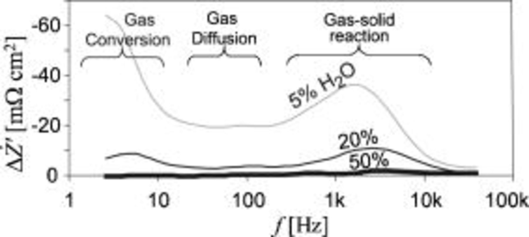
Figure 5.
 spectra recorded on an SOFC with a gas shift to the Ni/YSZ electrode from
  containing
 to
to  containing 5, 20, or
 . The bold line (50%) is a background noise measurement. All spectra are recorded with pure
  to the LSM/YSZ electrode.
The  spectra in Fig. 5 reveals three separable peaks, indicating that at least three different types of processes occur at the Ni/YSZ electrode and contribute to the impedance spectra. Again, the summit frequency can be found by drawing a straight line through the
  spectra peaks to the
  axis. The frequency at the intercept with the
  axis is the approximate summit frequency for the electrode arcs in
  containing
 . The frequencies are
  .
.
The gas-diffusion peak is not clearly visible in Fig. 5. To enhance the visibility of the gas-diffusion process, a H—D isotope experiment was made. First, a  impedance spectrum (
 containing 20%
  at a rate of
  ) was recorded and subsequently a
  spectrum (
 containing 20%
  at a rate of
  ) was recorded. Then, the gas was switched back to
  containing 20%
  supplied at a rate of
  and another
  spectrum was recorded. The LSM/YSZ electrode was fed with
 during the entire recording sequence. An average, noise-reduced
  spectrum for these conditions is shown in Fig. 6.
  is the background noise of the
  spectrum and is a noise-reduced
  spectrum produced with the two
  spectra.
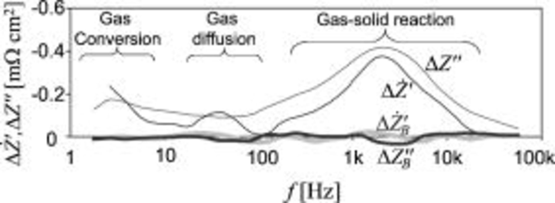
Figure 6.
 and
and  for a gas shift from
  containing
 to
to  containing
 .
.  and
and  are background-noise measures. Note that
  reveals three peaks while
  only reveals two and that the fluctuations of
  and
and  are of similar magnitude.
It might be argued that  is an equally good indicator of the summit frequency of a given process. Hence, for comparison, the average noise-reduced
  is also plotted in Fig. 6.
  is the noise-reduced uncertainty measure of
  using the first and second
  spectra. The three observed peaks in the
  spectrum are discussed in the next section. Note that the gas-diffusion peak is only observed with
  and that the fluctuations of
  and
and  are of similar magnitude.
Discussion
The  spectra in Fig. 4 reveal three identifiable peaks. Using a three-electrode setup, Jorgensen and Mogensen have reported that up to five different processes may contribute to the LSM/YSZ electrode.5 Barfod et al. investigated a symmetrical cell with LSM/YSZ electrodes on either side of the YSZ electrode.6 Three separable arcs were found in the impedance spectra with summit frequencies in good agreement with the low-, medium-, and high-frequency peaks in Fig. 4. The arc with a summit frequency of
  was ascribed to oxygen-intermediate transport in the LSM/YSZ structure near the electrode-electrolyte interface, the arc with a summit frequency of
  to dissociative adsorbtion/desorbtion of
  and transfer of species across the TPB, and the low-frequency arc
  to gas diffusion.5, 6
As the LSM/YSZ electrode is relatively thin on commercial cells  , gas-diffusion limitation is expected to be limited.6 It is instead suggested that the observed low-frequency peak is due to gas conversion in the gas-distributor plate on top of the electrode. When pure
  is fed to the LSM/YSZ electrode the gas-conversion arc disappears because the
  partial pressure is constant and equal to the total pressure.
Three separable arcs have previously been observed in impedance spectra recorded on the Ni/YSZ electrode in a three-electrode setup.7–10 The summit frequencies were reported as  for the low-frequency arc,
  for the medium-frequency arc, and
  for the high-frequency arc. The low-frequency arc was attributed to gas conversion8 and the medium-frequency arc was attributed to gas diffusion.9 The high-frequency arc has been found in a number of Ni/YSZ electrode setups.10 A gas–solid (desorption, absorption, dissociation) or solid-solid (surface diffusion, ion transfer across the double layer) reaction has been proposed for this electrode arc.7, 10 The three observed arcs are in good correspondence with the gas conversion, the gas diffusion, and the gas–solid reactionpeak observed in the
  spectra in Fig. 5 and 6.
In Fig. 5 the gas-diffusion peak is small compared to the gas-conversion and the gas–solid reaction peaks. In Fig. 6, the isotope exchange should not affect the gas-conversion arc. This explains why in Fig. 6 the gas-conversion peak is smaller, relative to the gas-diffusion peak. The reason why the gas-conversion peak is observed is possibly due to some small calibration error in the feed gas-flow rate when shifting from  to
to  . Alternatively, it may be that the equalization of the partial pressure of reactants in the gas volume to some degree involves gas diffusion.8
The  gas–solid peak in Fig. 6 seems to be well separated from the other peaks (no overlap). Hence, the peak may represent a time-invariant shift of the involved process. If the process that is responsible for the peak is adsorption or desorption of
  or
or  , a change in the active surface area would result in a time-invariant peak. From classical statistical mechanics it is predicted that the conductivity of
  in a solid is
  that of
  because the "attempt frequency" scales with
  , where
  is the mass of the isotope.17 At
  the ratio between the
  and
and  conductivity,
  , in a number of proton conductors has been observed to vary from
  to
to  .18
.18  and
and  diffusion in single-crystal Ni between 400 and
  has been investigated by Katz et al.19 The diffusion coefficient was found to decrease about 20% at
  when shifting from
  to
to  . Hence, a substitution of
  with
with  is likely to cause a decrease in the active surface area (the extension of the TPB) of the electrode, which would cause the observed gas–solid
  spectrum peak for the Ni/YSZ electrode reaction.
As discussed in the Appendix, the  spectrum provides a better resolution of the individual process contributions than a
  spectrum because it yields sharper and better-defined peaks around
  , the characteristic frequency for the impedance element
  . This is confirmed experimentally in Fig. 6, where the
  spectrum reveals the gas-diffusion peak in contrast to the
  spectrum.
The presented method to analyze differences in impedance spectra by variation of test conditions may be applied to other electrochemical devices, because it enables a selective study of process contributions to the impedance.
Conclusion
An SOFC was investigated based on differences in impedance spectra due to a change of operating parameters. Plotting the difference in the derivative with respect to  of the real part of the impedance is shown to be helpful in separating processes that overlap in impedance spectra. The produced
  spectra revealed three identifiable peaks at the LSM/YSZ electrode and three at the Ni/YSZ electrode. Each peak in the
  spectra corresponds to a change in a process that contributes to the impedance spectra.
The three  spectrum peaks observed at the LSM/YSZ electrode had peak frequencies around
  at
at  . This is in good agreement with previous findings in a three-electrode setup and a symmetrical-cell setup.5, 6
The Ni/YSZ electrode has previously been investigated in a three-electrode setup where a gas-conversion arc7, 8  , a gas-diffusion arc9
  , and a gas–solid or solid–solid arc9, 10
  were found. This is in good correspondence with the observed
  spectrum peaks, which had peak frequencies at
  .
.
Evidence for gas diffusion at the Ni/YSZ electrode was revealed in an isotope experiment where hydrogen was exchanged with deuterium. The produced  spectrum reveals a peak around
  . No evidence for diffusion was found in a
  spectrum. The enhanced resolution of processes in a
  spectrum compared with a
  spectrum is discussed in the appendix.
Acknowledgments
The authors thank the Fuel Cell and Solid State Department at Risø National Laboratory, Technical University of Denmark (DK), the Danish Energy Authority via the SERC project, contract no. 2104-06-0011 , and the European Commission via the  project, contract no. FP6-503765 for interest and financial support.
Risø National Laboratory assisted in meeting the publication costs of this article.
: Appendix
Below we calculate  and
and  for an
  circuit, an
  circuit, and a Gerischer element. After this, some discussion on
  follows, and finally an example of a
  spectrum is given.
Appendix. (RC) circuit
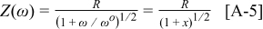
The impedance,  , for an
  circuit where
  is the angular frequency is given as

where  and
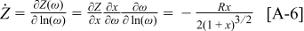
and  . We can now find the derivative with respect to
  as
as

Appendix. (RQ) circuit
The impedance,  , of an
  circuit, where
  is a constant-phase element with the impedance
  , is given as

where  and
and  .
.
The derivative with respect to  can be found as


Appendix. Gerischer element
The impedance for a Gerischer element may be written as
and the derivative with respect to  is found as
For the  element, separating into real and imaginary parts yields
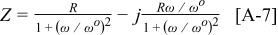
and
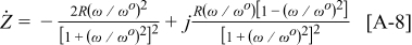
From Eq. 7, 8 it is seen that
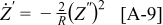
where  is the real part of
  and
and  is the imaginary part of
  . This explains why
  produces a sharper and more well-defined peak than
  . From Eq. 9 it is also seen that
  and
and  has a maximum (or minimum) at the same frequency. Taking the derivative of Eq. 7 with respect to ω, this frequency can be shown to be
  . Figure A-1 shows a plot of
  and
and  for an
  and the
  and
and  elements, given the values in Table I, condition A.
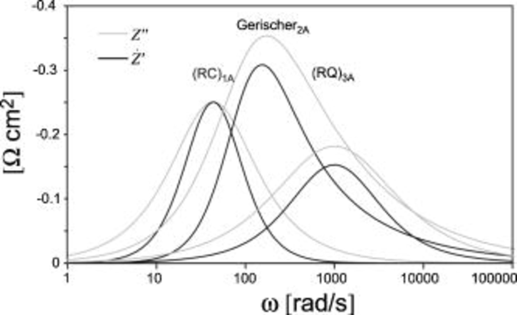
Figure 7.
 and
and  for
for  , a
, a  , and an
  , with the values specified in Table I, condition A. Note that
  produces sharper and more well-defined peaks than
  .
.
Table I. Values of the circuit elements.
| Circuit element | Parameter | Condition A | Condition B |
|---|---|---|---|
 element element |
 
| 0.5 | 0.53 |
 (rad/s) (rad/s) | 1000 | 1000 | |

| 0.8 | 0.8 | |
 element element |
 
| 1 | 1.1 |
 (rad/s) (rad/s) | 100 | 90.9 | |
 element element |
 
| 0.5 | 0.5 |
 (rad/s) (rad/s) | 43 | 40 |
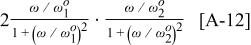
In general, an impedance spectrum is a sum of responses from several processes with different characteristic time constants. For simplicity, let us examine the response arising from two  in series, which we shall denote
  and
and  .
.
For such a circuit we can find
where  for
for  and
and  for
for  . If
. If  , a
, a  vs
vs  graph produces two overlapping peaks. We can also find
which also gives two peaks in a Bode plot, but the peaks are not as well separated as for  . Taking the square of Eq. 11 does not result in well-separated peaks in a Bode plot due to the formation of a cross term of the form
Now assume that an operation parameter Ψ is changed from condition A to B such that  is affected but
  remains constant. It then follows that
  is given as

If  , Eq. 13 can be further simplified to give
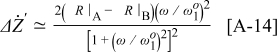
Comparing the real part of Eq. 8, 14, it is seen that  produces a peak with similar shape to the
  peak shown in Fig. A-1 with center at
  , but rescaled with a factor
  . Given the same assumptions as for the calculation of
  ,
,  can be found as
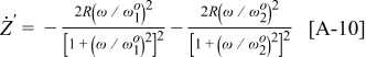
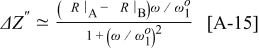
which produces a peak with a similar shape to the  peak shown in Fig. A-1 with center at
  , but rescaled with a factor
  . Looking at Eq. A-3 through A-6, it is clear that if
  is preserved, the peak shape is preserved. From Fig. A-1 it is then seen that a time-invariant (i.e.,
  -preserving)
  spectrum (from a single impedance element) only attains positive or negative values (and not both positive and negative values.)
Figure A-2 presents  and
and  for an
  , a Gerischer, and an
  element in series, undergoing a change in Ψ from condition A to B. The elements are referred to as
  ,
,  , and
, and  , and the parameter values for the elements are specified in Table I.
  undergoes a time-invariant change,
  undergoes a resistive change, and
  undergoes a capacitive change. Note that the three peaks are better resolved in the
  spectrum than in the
  spectrum.
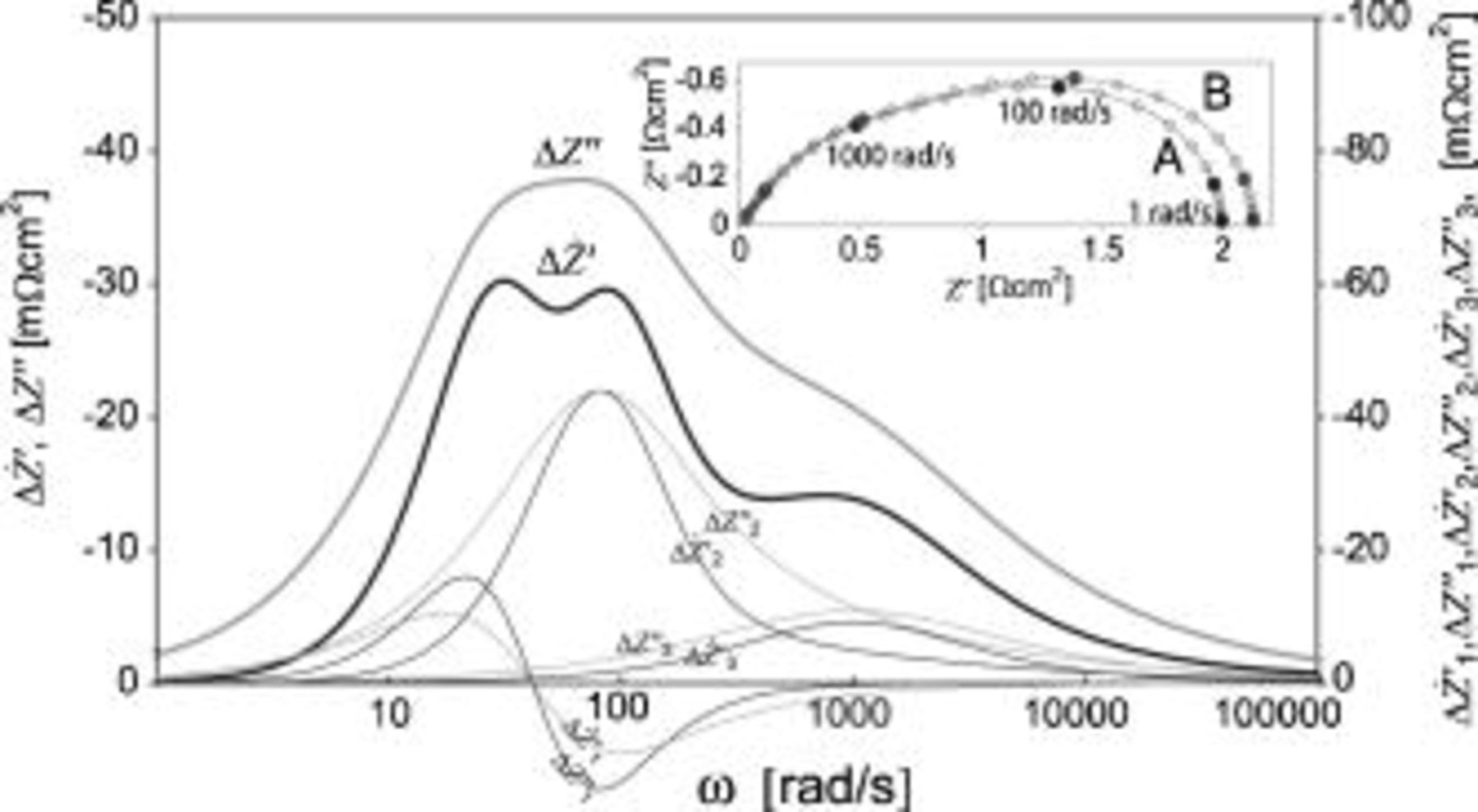
Figure 8.
 and
and  for
for  ,
,  , and
, and  in series, undergoing a change in Ψ from condition A to B as specified in Table I. The thin lines are
  and
and  for the individual elements. The inset is a plot of the impedance of
  ,
,  , and
, and  in series at condition A and B.
Footnotes
- c
For simplicity, the high-frequency peak is referred to as a gas–solid reaction.