
Abstract
Present solid oxide fuel cells (SOFCs) use complex materials to provide (i) sufficient stability and support, (ii) electronic, ionic, and mass transport, and (iii) electrocatalytic activity. However, there is a limited quantitative understanding of the effect of the SOFC's three dimensional (3D) nano/microstructure on electronic, ionic, and mass-transfer-related losses. Here, a nondestructive tomographic imaging technique at 38.5 nm spatial resolution is used along with numerical models to examine the phase and pore networks within an SOFC anode and to provide insight into the heterogeneous microstructure's contributions to the origins of transport-related losses. The microstructure produces substantial localized structure-induced losses, with approximately 50% of those losses arising from phase cross-sectional diameters of  or less.
Export citation and abstract BibTeX RIS
Increasing global power demands and environmental concerns have placed growing interest in the development of efficient, scalable, economic, portable, high energy density, and fuel flexible power sources.1–3 The solid oxide fuel cell (SOFC) is a promising candidate,2–5 where present SOFCs use complex material combinations and structures to facilitate the (i) selective transport of electrons, oxide anions, and fuel/oxidant, (ii) enhanced electrocatalytic/catalytic activity, (iii) stability, and (iv) structural support.4–9 Although the SOFC offers numerous advantages and opportunities, most of these opportunities stem from the use of a solid electrolyte that supports oxide anion  transport and medium to high temperature operations (e.g.,
  ). This combination provides favorable kinetics and transport properties,4, 5, 10 quality heat for secondary thermodynamic cycles,2–4, 10 and fuel flexibility that includes coal- and bio-derived fuel variants.5–7 However, present SOFCs are susceptible to degradation via several mechanisms related to the physiochemical behavior of the materials used and operational conditions, including contaminants in the mentioned fuels.6–8, 11, 12 Mitigation with alternative materials5–8 and operational conditions6, 8, 10 has shown promise but less favorable performance. Underlying the cell performance and its degradation are the complex structures that must facilitate the described selective transport processes, enhanced electrocatalytic/catalytic activity, stability, and structural support.4–9 These requirements pose fundamental constraints on the SOFC and require further exploration.
Many of the mechanisms that govern transport and degradation in the SOFC occur at the nano/micrometer length scales of the heterogeneous structure.9 Therefore, it is necessary to understand transport processes at these dimensions, but accurate three-dimensional (3D) descriptions of the nano/microstructure are difficult to obtain.13 Recent stereological studies have demonstrated high resolution and phase-specific 3D reconstruction and characterization of SOFC electrodes using a focused ion beam mill with a scanning electron microscope (FIB-SEM).14–17 Other analyses have used particle packing methods to replicate the fuel cell structure,18 but these methods have difficulty in validating that real structures are uniquely replicated. An approach that combines high resolution, nondestructive 3D imaging of the SOFC pore/phase structure with complementary characterization and analysis of transport processes within the microstructure is needed. In this study, a nondestructive imaging method that uses a full-field transmission X-ray microscope (TXM) for the direct imaging of a porous Ni, yttria-stabilized zirconia (YSZ) anode is demonstrated and used with detailed computational modeling to examine transport processes and losses within the SOFC's pore and Ni/YSZ phase structures.
Experimental
Sample preparation
The TXM-based X-ray computed tomography (XCT) measurements that are reported in this work consider a section of an anode-supported microtubular SOFC provided by Adaptive Materials, Inc. (Ann Arbor, MI). This section was taken from a fractured SOFC sample that did not have a cathode or current collector at the time of sectioning. A region within the interior of the sample, several microns from the fracture surface, was used for segmentation and analysis in the proceeding sections. This was done to avoid capturing surface effects from the fracture. Despite the exclusion of the cathode and current collectors, the SOFC sample used is a common form of the microtubular SOFC. It is composed of a porous Ni, YSZ cermet (i.e., ceramic–metal mixture) anode on a thin-film YSZ electrolyte. An 8 mol %  -stabilized
  form of YSZ was used in both the anode cermet and bulk electrolyte. The SOFC sample segment examined in this study was taken from the region containing the anode–electrolyte interface and approximately midway down the lengthwise direction of the tubular cell. This region was selected because of the importance of the heterogeneous elemental phase structure in these regions and their unique properties. The bulk regions of the sample used in this study have a pore volume fraction or porosity (i.e., the ratio of the pore to the total sample volume) of approximately 32%. The volumetric ratio of Ni and YSZ was nearly even in the bulk sample.
Full-field TXM measurements
To perform element-specific 3D imaging, a TXM at beamline 32-ID-C of the Advanced Photon Source at the Argonne National Laboratory19, 20 was used to carry out spectroscopic XCT measurements at a spatial resolution of 38.5 nm.21, 22 A schematic of the experimental setup is provided in Fig. 1. Monochromatic X-rays were produced using a cryogenically cooled, double-bounced Si(111) monochromator and double-reflection vertical harmonic rejection mirrors. An elliptical capillary condenser (73 mm in length and with an inner diameter ranging from 0.90 to 0.84 mm) was used to focus the incident X-rays on a sample. A gold (Au) Fresnel zone plate with a 45 nm outmost-zone width and 900 nm thickness was used as an objective lens to produce a magnified image of the sample on an optically coupled high resolution charge-coupled device (CCD) system. The high resolution CCD system consisted of a CsI scintillation screen, a visible-light objective lens (20×), a tube lens, and a  CCD detector with a
  size. A
  thick Au beam stop attached to the capillary and a
  diameter pinhole were used to block out the X-rays that were not reflected by the capillary. XCT measurements were performed by collecting 181 two-dimensional (2D) projections over 180° with a 50 ms per image measurement time. The XCT measurements were carried out within an interior region of the sample, away from the fracture surface. In this analysis, a 3D field of view for the XCT measurements, that is,
  , was achieved using the TXM. The instrument is capable of a
  field of view, and stitching methods were used for imaging and reconstructing volumes larger than the available field of view. In this study, 3D reconstruction was performed using a filtered back projection algorithm23 on a
  region of the imaged volume. Segmentation analysis was performed on an internal volume of
  in order to avoid edge effects.
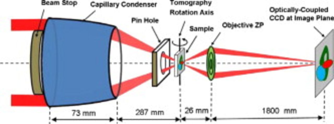
Figure 1. Schematic of the full-field TXM used for the experiment. The elliptical capillary condenser focuses the monochromatic X-rays from the synchrotron on the sample and the transmitted X-rays are magnified by a Fresnel zone plate objective lens on an optically coupled high resolution CCD system. The beam stop attached to the capillary blocks out the X-rays passing straight through the capillary without being reflected. The pinhole ensures that only the reflected X-rays can illuminate the sample. The X-ray computed tomography measurements were carried out by rotating the sample and collecting a series of 2D absorption contrast images. The schematic is not drawn to scale.
To achieve elemental sensitivity for Ni at the Ni–YSZ interface, microscopy experiments were carried out at 8.317 and 8.357 keV, corresponding to 16 eV below and 24 eV above the Ni K-edge (8.333 keV),24 respectively. The Ni elemental sensitivity at the Ni–YSZ interface supplements the sensitivity for the Ni/YSZ and pore interface that is distinguishable from measurements below the Ni K-edge. For example, for a 500 nm region of Ni, the X-ray absorption changes by 13.5% as the X-ray energy changes from 16 eV below to 24 eV above the Ni K-edge, providing a unique element-specific signature.24 The microscopy measurements performed in this study were carried out at a spatial resolution of 38.5 nm 20 and a field of view of  . This corresponds to an X-ray magnification factor of 81 and a pixel size of 8.0 nm. The change in the X-ray energy from 8.317 to 8.357 keV resulted in a negligible difference
  in the X-ray magnification.
Figure 2 shows TXM micrographs taken at 16 eV below (Fig. 2a) and 24 eV above (Fig. 2b) the Ni K-edge from a sample section of a porous Ni–YSZ anode supported on the dense YSZ electrolyte. Brighter features, such as the one indicated with the purple (upper right) arrow, are voids. Below the Ni K-edge, the two regions indicated by blue (upper left) and green (lower) arrows are similar in size and exhibit similar levels of absorption contrast. This demonstrates how imaging at a single energy would make it difficult to draw a concrete conclusion about the elemental nature of these regions. By comparison, only the micrograph taken above the Ni K-edge conveys that the grain indicated by the blue (upper left) arrow is Ni. As shown in Fig. 2c and 2d, which are projections of the 3D tomography data,25 the corresponding 3D reconstructed data sets provide unquestionable identification of the distinctive Ni, YSZ, and pore phases within the structure.
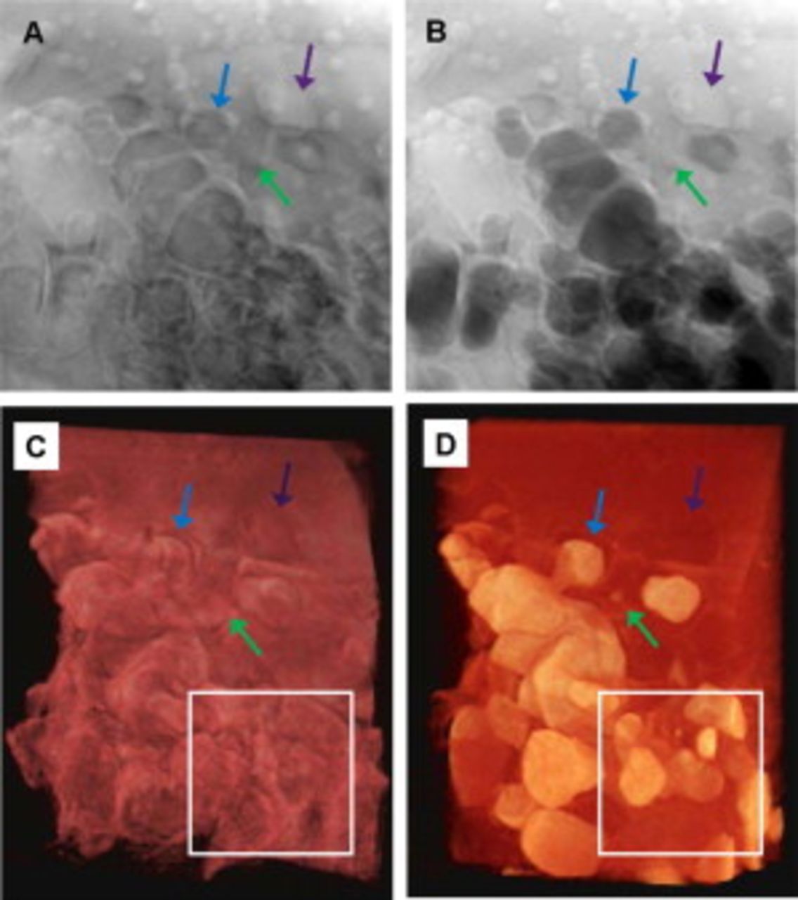
Figure 2. X-ray micrographs of the porous Ni–YSZ sample taken (a) 16 eV below and (b) 24 eV above the Ni K-edge of 8.333 keV with a spatial resolution of 38.5 nm. Darker tone indicates higher absorption. A projection of the reconstructed 3D tomography data at (c) 16 eV below and (d) 24 eV above Ni K-edge shows the same features in the sample, which are indicated by the colored arrows. Part of the reconstructed volume is shown with a lateral size of  . The white squares indicate the approximate region where segmentation analysis shown in Fig. 3 was performed.25
Segmentation and reconstruction
The digital reconstruction of the experimental TXM data began with the reduction of the measured data using a  binning process. This was performed to reduce the data size so that it was easily manageable by a single central processing unit personal computer. An accurate pixel representation of the sample data was available after the binning process. The postbinning pixels were 16 nm per side at a prescribed intensity, with stacks of individual transmission planes comprising the 3D structure. Initially, the details of the 3D morphology were rendered using the TXM 3D Viewer visualization software (Xradia, Inc., Concord, CA). Movies of the reconstruction provided in Ref. 25 show the 3D morphology of the SOFC anode sample with an X-ray energy of 24 eV above (8.357 keV) and 16 eV below (8.317 keV) the Ni K-edge of 8.333 keV,24 and the possibility to characterize phases using their absorption edges and the resolution detail and fidelity that the method permits.
The morphological rendering permits inspection of the XCT data; however, further processing was required to unambiguously represent the data so that it may be characterized, validated, and used in subsequent analyses. This was accomplished using a segmentation procedure. Segmentation was performed using ImageJ.26 The segmentation process began with the conversion of the 3D tomographic data into stacks of 2D TIFF images. These stacks are composed of individual 2D image planes or layers of the 3D structure that are stacked in the orthogonal (vertical) direction to form the full 3D morphology. The stacks were converted into 8-bit grayscale, and a  Gaussian blur filter was used to remove pixilation and enhance the edge contrast between the respective pore, Ni, and YSZ phases.
With the 8-bit grayscale stacks, the segmentation proceeded as follows. First, (i) alignment of the above and below Ni K-edge data was performed. Common and clearly defined geometric features visible in both the above and below K-edge data sets were used to triangulate the shift needed to align the two data sets. With the structures aligned, (ii) both data sets were cropped to the discrete volume considered in this study. This region was selected so that it was removed from the fracture surface and dense electrolyte. These requirements limited the volume available for the present study. To identify the discrete phases in the cropped structure, a threshold operation was used to reduce the 8-bit grayscale intensity data into a unique binary representation. The threshold operation was performed using (iii) above Ni K-edge data to identify the Ni-other regions and (iv) below K-edge data to identify the pore-other regions. In this study, the thresholds were selected by visual inspection of numerous 2D images within the stack from the corresponding above and below K-edge data sets. To complete this process, sharp changes in contrast at the respective phase boundaries were used to select the appropriate threshold values. Finally, (v) the YSZ regions were inferred by overlaying the post-threshold above and below Ni K-edge data sets (i.e., representative of the Ni-other and pore-other regions, respectively).
A modest limitation of this procedure is the visual inspection of individual slices used to set thresholds during the segmentation process; however, previous studies have used intrinsic data measured by independent experiments, such as the porosity from mercury intrusion porosimetry, to assist in the segmentation process.22 The use of this type of intrinsic data was not an option for the present study due to the small sample volume imaged, the sample's proximity to the anode–electrolyte interface which may maintain unique properties, and the inaccessibility of the independent pore/phase volume fractions with independent experimental methods. The development and examination of improved methods of reconstruction and segmentation will be pursued in future works.
Upon the completion of the segmentation threshold operation and alignment, the individual phase distinctions were given an unique integer type identifier (e.g., pore: 0, Ni: 1, and YSZ: 2). This provided a 3D structure comprised of voxels of finite size (i.e.,  ) and phase designation. For completeness, a voxel is defined as a 3D element representative of the structure. It can be considered as a 3D equivalent to a pixel representation.
Microstructural Characterization and Numerical Methods
Volume fraction
The Ni, YSZ, and pore volume fractions reported in this study are defined as the ratio of the sample volume contained by that phase to the total sample volume. Because the reconstructed 3D morphology is comprised of cubic voxels of a finite size and an individual phase designation (i.e., pore, Ni, or YSZ), voxel counting routines can be used to define volume fractions of each phase. This approach is consistent with previously reported methods.22
Tortuosity
The tortuosity of the Ni, YSZ, and pore phases of the sample were also examined. The tortuosities can be defined for all three of the principle Cartesian directions for the cubic segmented volumes studied. For clarity, the tortuosity is defined using a phenomenological 2D representation of a particular phase within the structure, which has been provided in Fig. 3. A single path, shown in white, represents a phase path that may exist in the sample. If the centerline of this path is followed, an effective length for this phase path,  , is found. The ratio of the effective path length to the nominal length of the sample volume,
  , allows tortuosity to be defined as
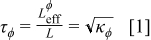
where τϕ is the tortuosity for the phase  . This definition has often been confused with the tortuosity factor, κϕ, that appears in the literature describing transport phenomena in porous media.27–32
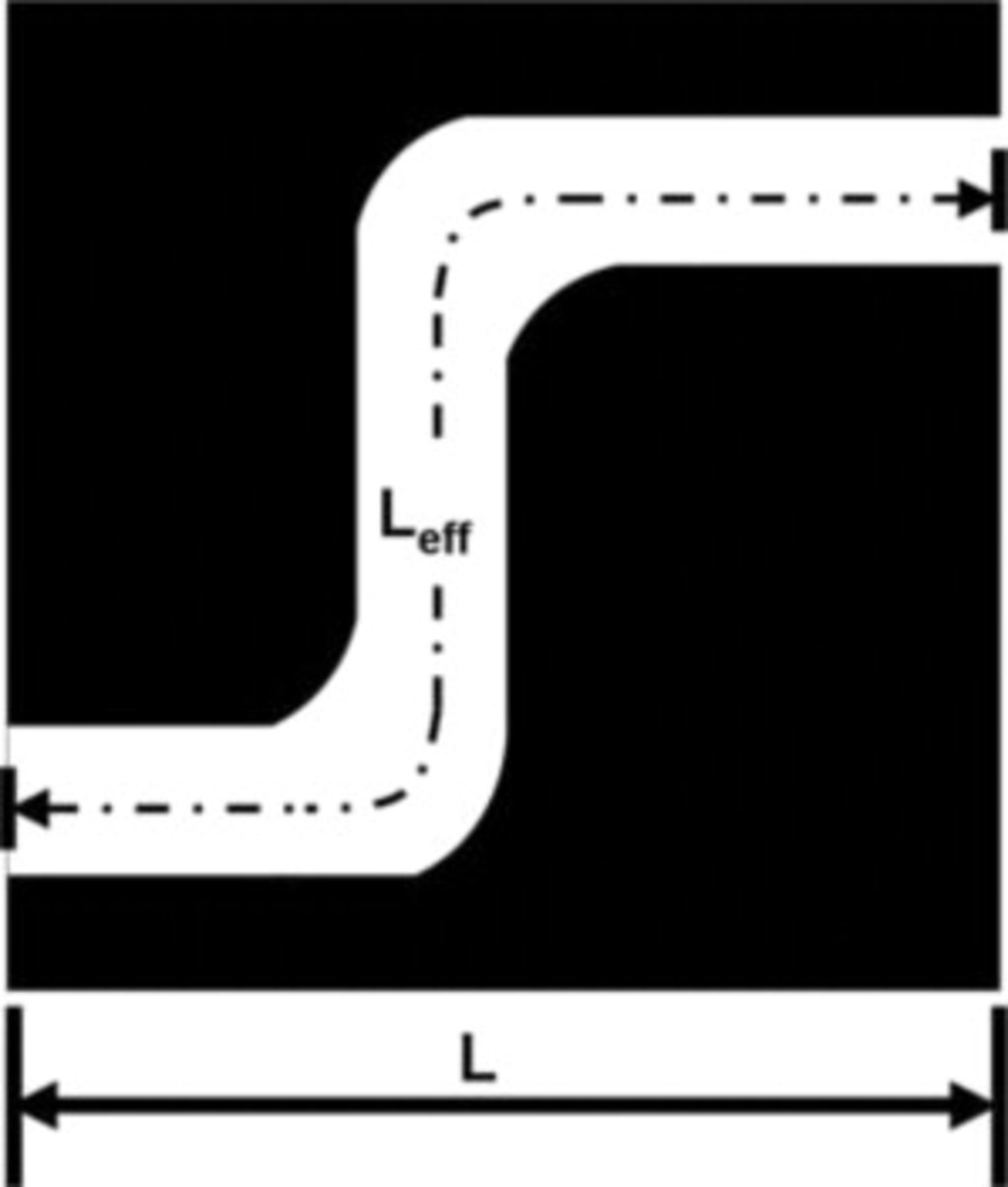
Figure 3. Conceptual representation of the effective  and nominal
  path lengths. The effective path length follows the centerline of the illustrated pathway being interrogated (shown in white). The solid black regions represent regions that are inaccessible by a given transport process occurring through the phase of interest. The tortuosity would be the ratio of the effective to nominal path length,
  .
.
The tortuosity of the individual Ni, YSZ, and pore phases within the sample were evaluated using a numerical method similar to that described by Joshi et al.33 Using the above description, the edge length of the medium  is known and the average effective path length
  is identified by solving Laplace's equation within the microstructure. The solution to Laplace's equation was used within this method to determine the effect of the structure on transport on a continuum level. By integrating the flux over the inlet area of the detailed domain, the solution was compared to an idealized one-dimensional solution that uses an empirical factor
  to represent the effects of the structure. Joshi et al.33 detailed that this empirical factor
  represents the effect of the pore structure on transport, but left the solution in terms of this factor. This factor is effectively a structural or material property. In this study, this definition was extended to study the solid Ni and YSZ phases. Also, tortuosity was explicitly identified by extending the definition of the factor
  to a physical interpretation of the structure. This interpretation is based upon a theoretical heuristic development, which is reported in an independent work discussing methods of characterization for heterogeneous systems with nano- to microstructures.34 The form identified in this study is consistent with what has been discussed and reported in several independent efforts.27–30 These efforts supported that the empirical factor
  could be correlated with the ratio of the volume fraction of the pore/phase in consideration of the square of the tortuosity shown in Eq. 1 for that same phase [i.e.,
  for the phase
  , maintaining a volume fraction of
  ].
].
Contiguity
The contiguity of the Ni, YSZ, and pore phases was examined. Interpretation of the contiguity, or percent volumetric connectivity, of the individual pore/elemental phases within a sample is important to understand the functional behavior of the system. This is important to the transport processes that must be supported and the interfaces between the independent phases and regions within the structure that must maintain sufficient contiguity to function.
To understand the contiguity, a 2D representation of its definition is provided in Fig. 4. A structure that is comprised of a single phase, or region, being examined (e.g., pore, Ni, or YSZ) is shown in white. In this structure, all remaining phases are shown in black. To interpret contiguity, the percentage of the total volume occupied by that phase that is disconnected within the structure would be considered noncontiguous for that phase. These volumes have been called out in Fig. 4 and are attributed to blind, or dead-end, paths from the left and right faces in addition to isolated regions for the phase being examined. The extension of these concepts and methods to the full 3D morphology is straightforward. This method is also used for the examination of two- and three-phase interfaces within the structure. Preliminary analysis of the contiguity of the pore phase has been reported in a previous study.22 The numeric methods for obtaining these measurements, as well as their verification, validation, and detailed interpretation, will be reported in the future.34

Figure 4. A 2D phenomenological representation of the contiguity of a segmented region of sample morphology is shown. Contiguity is being examined for the phase shown in white, and secondary phase/regions are shown in black. Isolated and noncontiguous regions are noted.
Two- and three-phase interfaces
The analyses of the volume-specific two- and three-phase interfaces within the segmented volume was a focus of this work. Specific attention was paid to the line that forms when the Ni, YSZ, and pore phases merge. Areas formed by the two-phase interfaces (i.e., Ni–YSZ, Ni–pore, and YSZ–pore) are also important. The values measured for the three-phase boundary (TPB) length and the two-phase area in the segmented volumes were examined in this work. These measurements were additionally considered in a modified form, which only considers contiguous regions of the structure. These measurements make use of the contiguity measurement methods discussed in the preceding section to remove noncontiguous regions.
The TPB length and the two-phase areas were evaluated using the digital representation of the segmented sample morphology. This is permitted by the binary representation of the structure in the form of voxels (i.e., 3D cubes of the isolated phase structure). On the basis of the reconstruction methodology, these voxels are of finite size (i.e., 16 nm per side) based upon the experimental setup and contain individual elemental phase designation.
To understand these measurements, phenomenological representations of the TPB line and the two-phase area interfaces for individual sets of voxels are provided in Fig. 5. In Fig. 5a, the unit line length that is formed by the union of voxels of the three constituent phases is observed. Figure 5b shows four voxels as they may appear in the reconstructed morphology. As the faces along which these voxels merge are inspected, two-phase interfaces can be distinguished. The areas are between two voxels of discrete phases and finite size  . Extending these isolated concepts to the full morphology, these interfaces were tracked and reported for the segmented volume. Details of the numeric method development, as well as the validation and verification of their use, are reported in a separate study.34
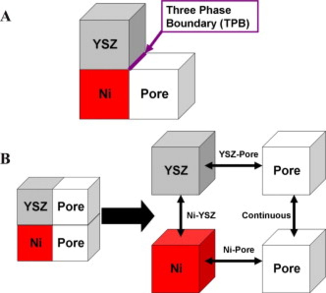
Figure 5. Conceptual representation of the phase interfaces possible within the reconstructed morphology. The cubes shown in these figures represent the voxels that comprise the reconstructed morphology that are of an individual phase designation and finite size as determined by the experimental setup and reconstruction processes. (a) The TPB line occurring at the union of three voxels of unique phase and (b) the two-phase interfacial areas at the faces of two voxels with different elemental phase designations.
Pore/phase size distributions
The phase-specific volumetric dependences of the reconstructed sample morphology were examined using numerical methods derived from a combination of the lattice Boltzmann method (LBM) spatial discretization scheme and a ray-shooting method. This method was used to tabulate the characteristic diameters within the segmented morphology so that a pore/phase size distribution (PSD) could be developed to quantitatively characterize the detailed sample morphology. The methods that have been developed and used in this study are related to other methods that have been reported (e.g., using chord length and correlation analysis), such as in Ref. 35–38, but are unique in development and practice.
The ray-shooting method in this study uses the 3D 19-velocity vector LBM routine.39, 40 In this discretization, each voxel has an associated 19-direction vector set including the local zero at the voxel center. Within the LBM algorithm, this vector set is interpreted as a velocity-space discretization, but it also provides a self-consistent set of direction vectors that are used for this study. The spatial discretization is used to simplify the analysis of the digital structure by limiting the direction that is considered. A 2D nine-direction (i.e., velocity) representation of this discretization is provided in Fig. 6a.
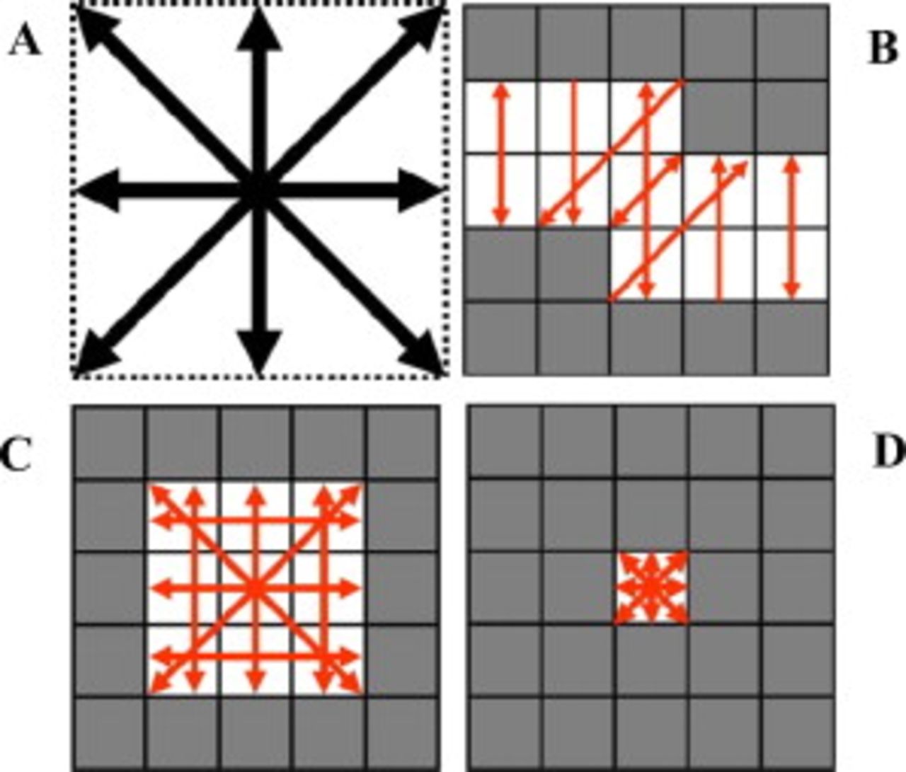
Figure 6. A conceptual representation of the LBM discretization scheme that is to examine the considered structures using the developed ray-tracing procedure is provided. (a) A 2D nine-direction representation of the LBM discretization is shown for simplicity, where a complementary 3D 19-direction set is actually used for this measurement. This set of finite direction vectors lying at every voxel within the structure is used to identify characteristic lengths or diameters. In (b), a 2D section running along a hypothetical pore/phase path centerline is shown. Rays at each voxel interface is launched using the LBM discretization, where the ray termination is indicated by a single arrowhead. Double arrowheads indicate a ray terminating on each edge of the path. Similarly, if the cross section of such a path is examined, (c) large and (d) small cross sections demonstrate that more rays are tabulated for a larger pore/phase cross section. The distribution functions formed using this data are developed in such a manner to treat these distinctions.
The 3D version of the spatial discretization shown in Fig. 6a consistently lies and connects through every voxel in the structure. Those that lie at the phase interface are of interest. The geometric data file is iteratively searched for the phase interface, including the pore/phase that is being examined. Voxels lying at the interface serve as launch points for individual rays that are used to map the structure. As a phase interface is identified, the 18 neighbors that share a face, edge, or corner to the voxel on the phase interface are examined to identify the normal direction from the interface. This normal direction corresponds to one of the 19 directions of the spatial discretization. Using the interface as a launch point, a ray can be tracked through the phase being examined until a second interface is reached. The length of the ray path, measured in voxels, is tacked and appended to a table. The table of ray lengths is used during the postprocessing analysis. This process continues through the geometric input file until the full structure has been examined.
A 2D representation of the ray-shooting process down the length of a pore/phase path (i.e., following the centerline) is provided in Fig. 6b. Likewise, Fig. 6c and 6d provides the cross section of a conceptual pore/phase path of unique diameter. In Fig. 6b, 6c and 6d, the dark gray squares are 2D representations of the voxels of secondary pore/phase regions, whereas the white squares are representations of the voxels of the phase being examined. In these figures, the slender arrows traversing the path are representative of rays that would have been launched by the described method. The head of these arrows represents the termination of a ray. Double-headed arrows indicate that there are two ray terminations; one from each of the respective ends of that path. As the structure is examined, a single ray is shot for each voxel along the respective phase interfaces. Although simplified by the 2D representation, both the convex and concave corners also maintain a ray at a 45° angle. Similar scenarios present themselves for the full 3D structure. As observed in Fig. 6c and 6d, depending upon the path cross section, different counts of rays can be anticipated. These rays also have unique lengths. The PSDs used in this study take the tabulated ray lengths and use them to interpret the details of the microstructure. Power spectrum theory is used in this effort, and full details regarding this development will be published in a separate work.41
Physically, the PSDs developed provide the volumetric contribution of pore/phase regions within the morphology that are described by a given pore/phase diameter  . The PSD is defined such that these contributions are provided over a defined bin width of differential diameter
  , and the magnitude is representative of the volume of all regions within
  of a given
  in the detailed, phase-specific morphology. The volume associated with each diameter was defined relative to the total volume of the segmented region studied, effectively normalizing it to the volume fraction that the phase occupies. Although this PSD is described in terms of pore/phase diameters, this measure of characteristic length is not uniquely defined to a circular cross section. It should be thought of as related to the cross-sectional area of a region of a given phase (i.e.,
  ) and is therefore more representative of a characteristic cross-sectional length or hydraulic diameter.
The developed PSD takes on the discrete form of a distribution function
where  is the PSD and takes on the units of inverse length
  . This function describes the magnitude of the volume fraction of the pore/phase ϕ associated with regions of diameter
  within a differential diameter of
  . The differential diameter
  represents the histogram bin width. By definition, this distribution function returns the total pore/phase volume fraction,
  , when integrated over all diameters

where the integration is shown in both continuous and discrete forms. Because each PSD represents a discrete analysis, it is distributed into M-bins, which represent the ratio of the number of rays associated with an individual bin,  , relative to the differential diameter,
  , representing the bin width. This represents a distribution,
  , and maintains units of inverse length (i.e., number or rays in bin
  within the bin width of
  divided by the bin width
  ). In Eq. 2, δ is the voxel length used during the examination of the sample volume. By performing a piecewise cumulative integration, as shown in Eq. 3, the cumulative volume fraction of a given phase with increasing diameter is also considered. Validation and verification of the method were performed using simplified cases and limiting conditions attributed to the structure during the theoretical development. Details on the theoretical development of the PSD, its validation and verification, as well as the numeric ray-shooting method used to tabulate the characteristic diameters of the structure will be reported in Ref. 41.
Transport discretization and solution methods
Transport processes were also examined in this study using a geometric file that was created using a segmented region of the reconstructed tomography data that describes the sample's morphology. For these studies, an LBM was used to examine transport processes because of its capability to capture the appropriate physics, amenability to complex geometric structures, and use of a regular mesh with high grid independence. Detailed reviews on the governing theory and implementation, boundary conditions, and scalability are widely available.42–54 The implementation used in this study resembles those reported in previous studies,43, 55, 56 with consideration of the second-order zero flux boundary condition at the impermeable phase interfaces.45, 57 The extension of these methods to consider the continuum electronic and ionic conduction processes was completed on the basis of the ability to recover a solution to Laplace's equation when evaluating molar mass transfer in the limit of two species in the absence of viscous flow.43 Scaling of the diffusion solutions was treated as an analogous form to those reported for mass transport in independent studies, which also provided thorough reviews of verification and validation of the numeric methods.33, 43, 56
The analyses of the three independent transport processes of binary mass transfer (i.e.,  ), ionic charge transfer, and electronic charge transfer were performed on an SGI Altix 3700 high performance computing cluster. These cases were run using eight 1.5 GHz Intel Itanium-2 processors. Parallelization was completed using a vertical domain decomposition scheme with interprocessor communications performed via message passing interface routines. All codes were written in Fortran. Solutions were examined under steady-state isothermal conditions. Convergence was monitored using the total and species conservation principles. Solutions were considered converged when error in the species balance was less than 1%. The time to reach a steady-state solution ranged from the order of 3 days to 3 weeks depending upon the complexity of the structure and transport properties. Bulk values for
  molecular diffusivity
  , Ni electronic conductivity
  , and YSZ ionic conductivity (4.28 S/m) were taken using values reported for
  within the literature.58–61
Data postprocessing and visualization were completed on a single-processor personal computer. The scalar fields and fluxes are available products of the numeric methods; additional postprocessing was required to identify the net resistive losses due to Joule heating. This analysis was accomplished by using the flux outputs from the LBM analysis at each voxel within the structure. The resistive loss or Joule heating in a voxel at a position  can be described as

where  is the heat liberated, due to Joule heating, per unit volume in
  at the given voxel position
  , ρ is the material's resistivity in
  , and
, and  , the current density in the
  -direction in
  , at the corresponding voxel location. The net rate of heat released at position
  can be formulated by multiplying Eq. 4 by the differential volume attributed to an individual voxel. The net resistive losses for the ionic (YSZ) and electronic (Ni) analyses performed in this study with a superficial current density of
  were
were  and
and  , respectively. Both are defined with respect to the total volume of the domain.
The scalar field that comprises these resistive losses was used to perform the 3D visualization and analysis of the local heat released. Additionally, the heat released for the Ni and YSZ structures was also written to files that mirror the respective geometric structural files for subsequent analysis. These data files maintain a scalar heat release quantity at each voxel position in the digital structure, representative of the heat released over the voxel volume. These files were used during the development reported in the next section.
Microstructure-induced resistive-loss distribution
Among the developments reported in this study is a microstructure-induced resistive-loss distribution (MRD), which quantitatively describes the microstructure's contributions to resistive losses in the form of Joule heating (i.e., resistive losses) within the electronic (Ni) and ionic (YSZ) carriers of the heterogeneous sample structure. Prior to providing details on the numeric description of the MRD, it is worth elaborating upon its physical interpretation and implication on this type of analysis. From a physical standpoint, it is understood that forcing a current through a narrow region results in increased resistive losses due to Joule heating. This loss is effectively associated with the thermodynamic irreversibility (i.e., entropy generation) of the conduction processes and has been known to be especially problematic in structures with constrictions (i.e., necked regions). In heterogeneous structures such as the SOFC anode, the implications of the detailed phase structure on these types of effects are difficult to quantitatively understand despite their importance.59 The MRD has been developed to provide a means of quantitative analysis that can unify the details of the heterogeneous structure with its contribution to resistive losses within the structure.
To understand the MRD, a resistive-loss distribution (RLD) is first introduced. The RLD describes the net resistive losses of the electronic (Ni) and ionic (YSZ) transport processes that are attributed to regions of the structure described by phase diameter  in units of energy (i.e., watts). This RLD coherently links the quantitative characterization of the phase/pore specific structure using the already described PSD functions to analyze the ionic and electronic transport processes in the YSZ and Ni phases. To do so, a complementary LBM-based ray-shooting method is used to interpret and tabulate the scalar resistive losses in the detailed microstructure as a complement to the characteristic pore/phase lengths. As shown in Eq. 5, the RLD uses this information to describe the net losses attributed to the charge-transfer processes as a function of phase diameter. However, as shown in Eq. 6, the MRD normalizes the RLD by the product of the material resistivity
  , the square of the superficial current density
  , and the sample volume being considered
  or
or  , which represents the resistive loss that would be observed in the same volume if it were entirely comprised of that particular phase (e.g., Ni or YSZ). This normalization permits a direct comparison of the effects of the detailed Ni and YSZ microstructures on their respective charge-transfer processes.
To perform the MRD and RLD analyses, the mean resistive losses associated with regions of phase diameter  within a differential diameter
  were determined using a similar ray-shooting methodology to that which was used to characterize the PSD functions. Complete details on this development will be available in Ref. 41. By using a consistent method to the PSD, the mean resistive loss for a region and the characteristic cross-sectional phase diameters used to develop the PSD could be coherently obtained. With this consistent definition, the mean resistive losses associated with a given phase diameter were tabulated for the considered structures and transport processes/conditions. Using this data, the RLD developed to interpret this data provides the net resistive loss associated with regions of diameter
  within a differential diameter
  , which represents the histogram bin width
where  is the RLD in
  . As shown,
  is the sum of the mean resistive losses in
  attributed to a given bin, and
  is the net resistive loss determined by the transport analysis in watts. In a similar manner to the PSD, the RLD is defined so that its integration over all diameters returns the net resistive loss
  that was observed in the segmented volume during the transport analysis.
Due to the large differences in bulk ionic (YSZ) and electronic (Ni) resistivities for the analyses completed, the RLD was further modified so that the effects of the microstructure could be separated from resistive effects attributed to the bulk materials, structures, and conditions. This resulted in the development of the MRD, which permits the resistive losses induced by the heterogeneous structures to be directly compared so that the effects of the microstructure can be understood. This was achieved by dividing Eq. 5 by the resistive losses attributed to a bulk region of the phase being considered at comparable conditions to negate these effects and effectively isolate microstructural contributions to the losses. The resistive losses attributed to bulk regions of the considered phase ϕ were defined as the product of the domain volume  , the square of the superficial current density
  (i.e., operation current density), and the bulk material resistivity ρϕ. This allows the MRD to be shown as
where  is the MRD describing the resistive losses induced by the microstructure in the considered volume and takes on the units of inverse length
  .
.
Results and Discussion
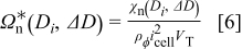
Using the methods described in the preceding sections, segmentation and reconstruction procedures were used to obtain the distinct Ni, YSZ, and pore phase regions within a  volume, as shown in Fig. 7a, validation of this reconstruction and segmentation discussed in Appendix
  , respectively.
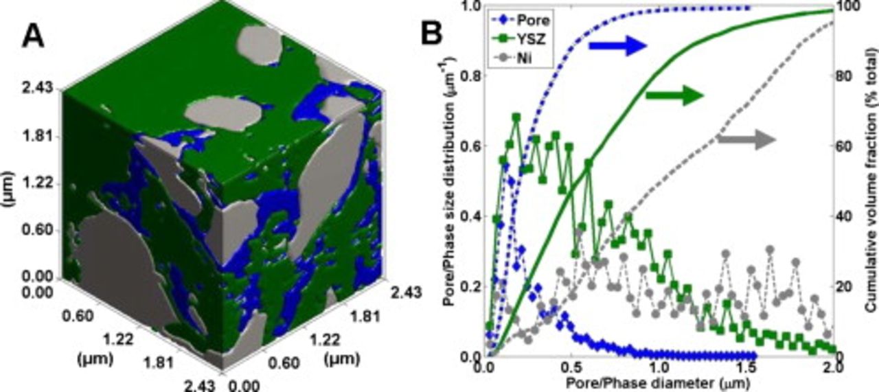
Figure 7. The phase-specific segmented volume is rendered, (a) showing the YSZ (green), Ni (gray), and pore (blue) regions. The relative pore/phase volumes associated with regions of a given pore/phase diameter in the structure are shown using a (b) PSD. The cumulative percentage of pore/YSZ/Ni volume is provided on the secondary axis.
A  subvolume of this reconstructed and segmented volume was further segmented for a more detailed analysis, with details on the volume fractions, tortuosity, and contiguity for the volume reported in Table I. This subvolume was used because of the segmented volume's proximity to the electrolyte interface and so that the computationally study of transport processes could be pursued. Because of its small size, this volume may not be representative of the full electrode.22, 62 For a property to be considered representative, it must be shown to be independent of the volume considered, which was not possible in this study. Boundary truncation effects may be at play for the small volume considered. Boundary truncation occurs as a result of the splicing of the real geometry. This truncation can skew the measured results with respect to what should be obtained for the bulk electrode.62 This can specifically affect properties such as the pore/phase contiguity, volume fraction, tortuosity, and interfaces with contiguous pathways through the structure. The
  volume can still be used to demonstrate the insights provided by the detailed characterization methods. These methods are amenable to larger volumes that may be shown to be representative. Additionally, the properties of this volume are given in the interest of providing a complete description of the volume considered. A more detailed description on the importance and implications of volume independence in heterogeneous structures is provided in Appendix
Table I. Quantitative analysis of the volume fraction, tortuosity in the principle Cartesian directions, and contiguity of the Ni phase, YSZ phase, and pore regions of a  segmented volume.
| Region ϕ |
 |
 |
 |
 | Contiguity (vol %) |
|---|---|---|---|---|---|
| Ni | 0.46 | 1.67 | 1.22 | 2.69 | 96.8 |
| YSZ | 0.36 | 2.24 | 1.44 | 1.71 | 99.4 |
| Pore | 0.18 | 1.33 | 1.23 |
 | 93.2 |
aDenotes anomalously high value, likely a numeric artifact of size of the segmented volume, anisotropy in the  -direction, and its proximity to the electrolyte interface.
Understanding this limitation for the present study, Fig. 8 shows results obtained for the study of the discrete mass, electronic, and ionic transport processes that occur in the anode/electrolyte interface region within the pore, Ni, and YSZ phases of the  segmented volume subjected to a
  current density.17, 59 Details on the validation, mass/charge conservation, and numeric methods are well documented.43 Electrochemical oxidation was neglected for this analysis, representing a phenomenological case where no electrical neutralization of the
  occurs within the volume. Constant transport coefficients at 1073 K were assumed, neglecting localized effects such as space charge, resistive intermediate YSZ and Ni phases, and noncontinuum transport; however, no empirical descriptions of the structure were necessary, permitting examination of the impact of the nano/microstructure on transport phenomena.
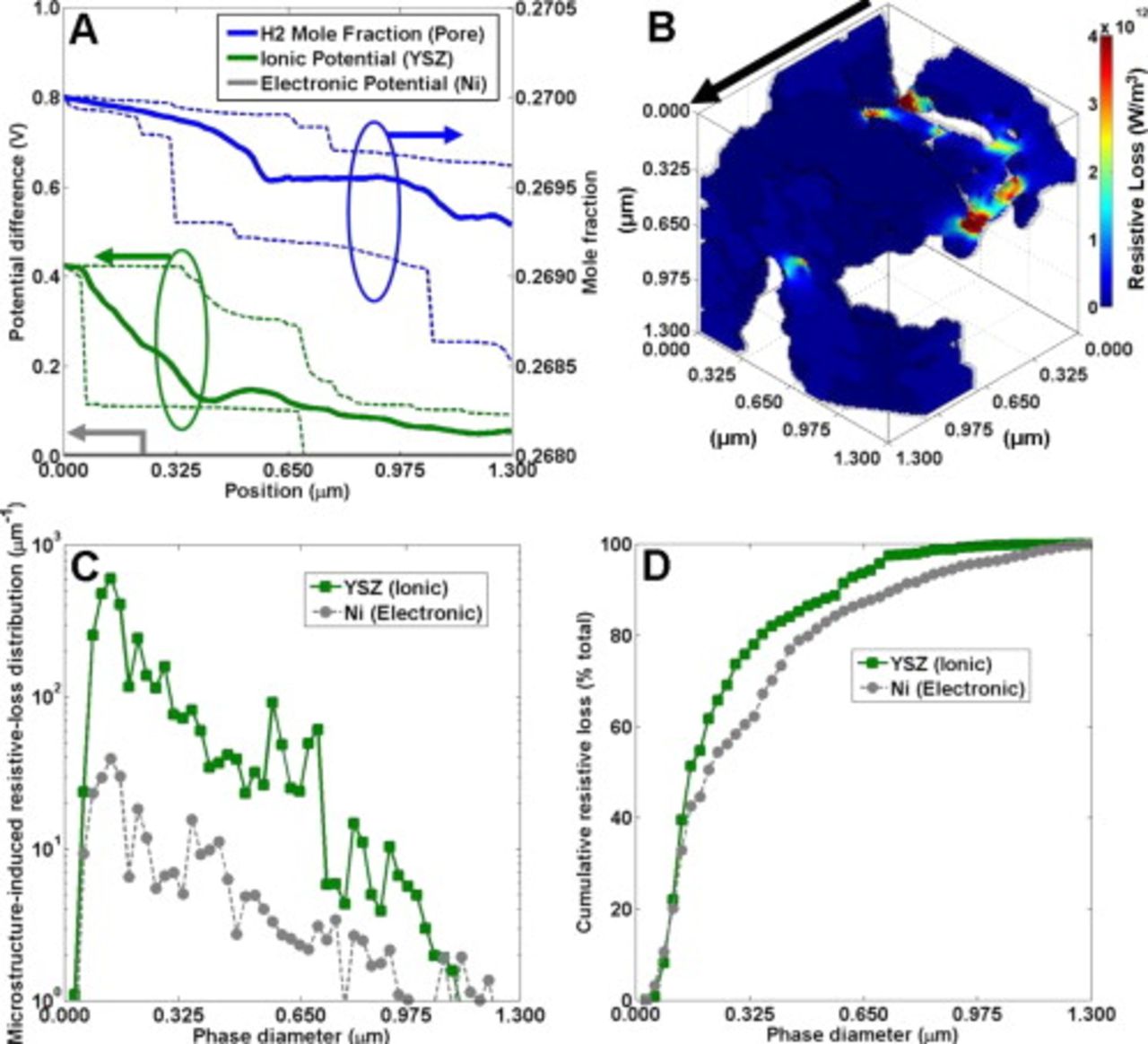
Figure 8. Transport processes in the SOFC anode segment at a current density of  and operating at 1073 K. (a) Variations in the hydrogen mole fraction (pore) and the ionic (YSZ) and electronic (Ni) potential differences are shown along the primary transport direction. Solid lines represent the mean values and the dashed lines represent the bounding in-plane variations. The primary transport direction is noted by the arrow in (b), which shows significant localized resistive losses in the YSZ phase. MRDs to the (c) ionic and electronic phases are described in terms of phase diameters, where the bulk material resistive contributions have been annulled. (d) The cumulative ionic and electronic resistive losses.
Figure 8a shows the mean ionic potential difference, electronic potential difference, and the hydrogen mole fraction along the primary transport direction as solid lines. The dashed lines bounding these trends provide their maximum/minimum in-plane values, demonstrating the considerable effect that the microstructure has on the local variation in mole fraction and potentials. Gradients in the transverse direction approach the mean gradients in the primary transport direction, thereby redirecting transport away from the primary direction, potentially resulting in increased losses within the fuel cell structure. For reference, the 3D plots of these hydrogen mole fraction (pore) and ionic potential (YSZ) distributions are provided in Fig. 9, which visually reflects these gradients. Focusing on localized variation in the YSZ and Ni phases, we observed large local losses in the constricted regions of the microstructure, indicated by red (online) in Fig. 8b. As much as an 210× and 30× increase in local ionic (YSZ) and electronic (Ni) current densities relative to the prescribed current density are observed, respectively.
Figure 9. 3D scalar distributions of the discrete transport studies performed within the segmented volume. Results correspond to total fluxes at a current density of  , temperature of 1073 K, and include the (a) hydrogen mole fraction in the pore phase and (b) ionic potential differences in the YSZ phase. Yellow and black circular fiducial marks denote a common geometric point. The arrows denote the primary transport direction.
To quantify the contributions of the nano- and microstructures to the ionic and electronic resistive losses, MRD is shown in Fig. 8c. The MRD quantifies the resistive losses in the structure as a function of a phase's cross-sectional diameters within the volume while negating the contributions from the bulk material resistivity, operational current density, and segment volume. This permits the MRD to provide a direct comparison of the microstructural contributions to the resistive losses for discrete regions and transport processes in the ionic (YSZ) and electronic (Ni) regions. The integration of the MRD across phase diameters in Fig. 8d is representative of cumulative resistive loss observed in the structure.
Several insights are apparent in Fig. 8c and 8d. Losses attributed to ionic transport (YSZ) outweigh those for the electronic transport (Ni) by more than 6 orders of magnitude when bulk material resistance effects are considered. However, the MRD in Fig. 8c shows that the details of the microstructure still play an important role even after bulk material resistance contributions have been annulled. Although both the electronic (Ni) and ionic (YSZ) phases see their most substantial losses at small phase diameters, YSZ consistently exhibits greater losses with up to 10× greater resistive loss at small diameters. Although intuition suggests that the smallest diameter would yield the largest losses, this study shows largest losses to be a combination with the volume attributed to that particular region diameter which is available for transport. The cumulative resistive losses exhibited by Ni and YSZ phases are similar. In fact, Fig. 8d shows approximately 50% of both the ionic and electronic resistive losses occurring in regions with diameters of  and less. At diameters greater than
  , Ni and YSZ exhibit similar cumulative resistive loss trends, but the cumulative resistive losses for the ionic transport separate and rise more rapidly due to a larger amount of small
  YSZ regions.
These observations suggest that improved manipulation of the YSZ structure may provide substantial performance improvements. Yet the electrochemical oxidation reaction, which neutralizes ionic flux extending into the anode and likely results in increased resistive loss,6 is not considered at this time. To consider these effects, parallel mass, electronic, and ionic transport processes would require explicit coupling through the details of the electrochemical oxidation reaction kinetics.6
The Ni, YSZ, and pore phases exhibit 96.8, 99.4, and 93.2% contiguity by volume, respectively. Had the oxidation and coupled transport processes been considered, sufficient contiguous transport pathways to the line forming the TPB for the participating species/regions are necessary. However, only 3% of all the TPB lines maintain contiguous or connected regions through each of the participating pore/phase regions. The small volume used in this study may have significantly contributed to the discrepancy between the absolute and contiguous TPB lengths. Boundary truncation62 of the individual phase contiguities, which are compounded in the contiguous TPB length measurement, may have resulted in the discrepancy between the absolute and contiguous TPB lengths. The results reported in this study are provided with independent measurements16, 17 in Appendix
Table II. Interface properties of a  segmented volume, including the two-phase interfacial area and TPB length. A modified form that only considers those interfaces with contiguous pathways through the participating regions of the structure is also provided.
| Interface | Area | Contiguous area | TPB length | Contiguous TPB length |
|---|---|---|---|---|
| Ni–YSZ |
 |
 | — | — |
| Ni–pore |
 |
 | — | — |
| YSZ–pore |
 |
 | — | — |
| Ni–YSZ–pore | — | — |
 |
 |
bThe contiguous TPB length may not be representative of the bulk heterogeneous electrode structure. The values reported here may be reduced due to a decreased contiguity of the participating regions due to boundary truncation effects resulting from the small sample volume.
Conclusions
The imaging and analysis of the SOFC pore/phase structure have provided insight into its complex nature. As TXM instrumentation capabilities improve, X-ray energies higher than 16 keV should become available, permitting elemental sensitivity for other important phases for the SOFC-containing elements such as Sr, Y, and Zr or more novel materials such as Cu and Mn being examined for enhanced stability in coal- and bio-derived fuels. The extension of these capabilities to in situ or parametric study of (i) unique materials, (ii) manufacturing methods, (iii) sintering/redox conditions, and (iv) operation conditions may provide considerable opportunities for enhancing our understanding of the role of nano/microstructures in SOFCs.
Acknowledgments
The authors K.N.G., A.A.P., J.R.I., and W.K.S.C. gratefully acknowledge the financial support from the Army Research Office Young Investigator Program (award 46964-CH-YIP), the National Science Foundation (award CBET-0828612), the Energy Frontier Research Center on Science Based Nano-Structure Design and Synthesis of Heterogeneous Functional Materials for Energy Systems funded by the U.S. Department of Energy, Office of Science, Office of Basic Energy Sciences (award DE-SC0001061), and the ASEE National Defense Science and Engineering Graduate Fellowship program. The authors thank Adaptive Materials, Inc. for the SOFC samples. Use of the Advanced Photon Source was supported by the U.S. Department of Energy, Office of Science, Office of Basic Energy Sciences, under contract no. DE-AC02-06CH11357 .
University of Connecticut assisted in meeting the publication costs of this article.
:
Appendix A Validation of Reconstruction and Characterization Methods
A validation of the reconstruction, segmentation, and quantitative characterization methods used in this study was necessary. To support these efforts, several aspects of the analysis were examined on an independent basis. Details on the segmented volume and analyses are provided in Tables I and II, which represent properties of the considered region.
This validation began with a comparison between the interfacial measurements and several measurements and estimates that have been reported. The limited sample volume considered and the unique properties of the sample make direct comparison of interfacial measurements difficult; it is not unreasonable to make general comparisons. To this extent, the TPB length and two-phase interfacial areas in Table II are reported in an absolute form (i.e.,  and
and  , respectively), and one that only considers regions that maintain contiguous pathways through the participating pore/phases to the interface (i.e.,
  and
and  , respectively). The TPB lengths (i.e.,
  and
and  ) and phase interfacial areas (i.e.,
  ,
,  ,
,  ,
,  ,
,  , and
, and  ) are identified in this study and compare well to those reported by Wilson et al. (i.e.,
  ,
,  ,
,  , and
, and  ).16, 17 Wilson et al. used an FIB-SEM to study the SOFC microstructure. In a subsequent study, Wilson and Barnett reported TPB lengths ranging from
  to
to  depending upon volume fractions and particle sizes used during fabrication, which compares favorably to this study.
Qualitatively, these interface values can also be compared to empirical predictions and estimates that have been deconvoluted from more complex experiments and stochastic theories.64–72 We examine several of these analyses here. Lee et al. suggested interfacial area values of  ,
,  , and
, and  for a sample with a comparable Ni content to those that were examined in this study using stereological methods with an optical microscope.64 Drescher et al. provided an interfacial area of Ni and the pore phase of
  through the use of a Brunauer, Emmett, and Teller adsorption analysis,65 where a Ni density of approximately
  was used to arrive at this figure using the reported measurements. DeCaluwe et al. used geometric considerations and experimental SOFC polarization curves to determine a TPB length of
  and interfacial areas on the order of
  for the Ni–pore and YSZ–pore interfaces.30 Similarly, percolation theory has often been used in the SOFC literature to estimate the TPB length and interfacial areas through considering the coordination of constituent spherical particles with a prescribed degree of contact.64–72 Using these types of methods, Costamagna et al. estimated Ni–YSZ interface areas70 ranging from
  to
to  , and Jeon et al. estimated a TPB length66 of approximately
  using this type of approach.
These values provide only a sampling of the analyses that have been reported using these types of approaches. Subsequently, the values identified can vary depending upon the assumed structure. Still, the comparable orders of magnitude that were observed provide further confidence in the reconstruction and analysis.
Further verification of the reconstructed and segmented structure can be obtained through the examination of the mean Ni and YSZ phase diameters determined with the PSD analysis. The volume-weighted mean YSZ and Ni diameters of 0.5 and  , respectively, are quite comparable to common particle sizes used during manufacturing.4 The mean pore diameter of
  is also reasonable, especially considering the segmented volume's proximity to the electrolyte interface.22, 73 Similarly, the pore/phase tortuosities reported in Table I are comparable to those that have been previously reported for multiphase 3D structures including SOFC anodes.16, 17, 22, 29, 31, 33, 73
:
Appendix B Heterogeneous Structure Analyses
The heterogeneous structures that were considered in this study can have some significant implications on the properties that have been reported. Because a small sample volume (as small as  ) was considered in this study, its properties (e.g., the phase volume fractions, tortuosities, etc.) may differ greatly from those in a neighboring region of the sample. This naturally includes a discrepancy from the properties of the bulk electrode structure. However, this does not imply that the properties associated with this volume are not important and have a considerable localized effect. A value that is representative of the broader structure is typically desired for the properties measured. However, due to the limited volumes available for analysis, reporting such a representative value is not possible here.
For complex heterogeneous structures, there is no guarantee that a value that is representative of the broader heterogeneous sample structure can be obtained; however, the values measured for these properties typically approach those that are representative of the bulk structure if a large enough volume is considered. Further treatise on the implications and treatment of these issues has been addressed in previous studies22 and are examined further in a supporting study.34, 41