
Abstract
Lithium-ion batteries (LIBs), which are increasingly employed for energy storage, should be reused whenever possible to mitigate resource depletion and environmental problems. This requires a nondestructive diagnostic method to assess their potential for reuse in terms of capacity reduction and power drop, which occurs with increased internal resistance. The diagnostic method should be fast and simplified with no need to adjust the temperature or state of charge (SOC) when classifying numerous LIBs. To develop such a method, we compiled 4,220 impedance measurements taken at temperatures ranging from −20 °C to 50 °C and SOCs from 0% to 100%. 18650-type cylindrical LIBs were used to construct a prediction model of the capacity or internal resistance via machine learning using the impedance, temperature, and open-circuit voltage, instead of the SOC. Through a strict selection of frequencies at which the impedances of used LIBs were measured, it was possible to simultaneously predict LIB capacity and internal resistance with high precision at any temperature or SOC after less than 1 min of impedance measurement. To enhance the generalization performance, three types of degraded LIBs were employed in the prediction model. Finally, this study demonstrated improved data prediction in the extrapolation area.
Export citation and abstract BibTeX RIS
Lithium-ion batteries (LIBs), which are primarily used in electric vehicles and as energy buffers for photovoltaics, are key devices for energy storage in sustainable societies. As LIBs contain rare metals such as Li, Co, and Ni, their reuse or recycling is important to combat resource depletion and environmental problems; however, this is hindered by many issues, including high costs. Therefore, to promote the reuse or recycling of used LIBs, diagnostic technology is required to fully evaluate the capacity reduction and power drop of LIBs that occur with an increase in internal resistance. Such a technique should be capable of assessing the degree of degradation in used LIBs at any state of charge (SOC) and temperature; otherwise, diagnosis would require time-consuming adjustments of SOC and temperature, which would necessitate the use of thermostats and charge/discharge devices. In addition, the diagnostic testing time should be as short as possible to allow the classification of multiple LIBs.
Previous studies have applied machine learning to various LIB prediction methods. 1–4 For example, Ng et al. 5 reviewed a variety of methods for predicting the capacities of degraded LIBs via machine learning. Moreover, several studies have investigated the correlation between the capacity and impedance of degraded LIBs. 6–10 For example, Schuster et al. 6 showed a correlation between capacity and impedance at 25 °C and an SOC of 50% using LIBs with calendric and/or cyclic aging. They also reported the importance of the ohmic resistance and typical internal resistance, Rpl + ct , obtained from the impedance for capacity prediction. Zhang et al. 7 also revealed a correlation between the capacity and impedance of LIBs with cyclic aging at 25 °C, as well as the importance of impedances at 17.80 Hz and 2.16 Hz for capacity prediction. However, these studies do not satisfy the above-mentioned diagnostic conditions, that is, the temperature and SOC for capacity prediction must be adjusted, and the generalization performance of the prediction for a variety of degradation processes remains unclear.
Therefore, this study proposes a nondestructive, rapid diagnostic system for LIB deterioration with good generalization performance. A conceptual drawing of the proposed diagnostic system is shown in Fig. 1. Measurement of the capacity of used LIBs requires a long time for charging and discharging at a low current rate (C-rate) to avoid the influence of polarization, for example, 10 h at 0.1 C. Therefore, we apply impedance to estimate the capacity because the measurement time for impedance is shorter than that for capacity. After measuring the impedance of the LIBs, the capacity is predicted using the measured impedance. The prediction model is constructed via machine learning using a database of impedances related to capacity, which is prepared in advance. The internal resistance and capacity are predicted simultaneously, followed by an evaluation of whether the LIBs can be reused or recycled (Fig. 1).

Figure 1. Conceptual drawing of the proposed diagnostic system for LIB deterioration.
Download figure:
Standard image High-resolution imagePredicting LIB capacity can be difficult as LIB deterioration can result from a complex interplay of various factors, 11,12 such as electrode material cracking and decomposition, 13,14 solid electrolyte interphase (SEI) growth, 15,16 and Li plating at the anode. 17–19 Previous studies have reported that three degradation modes are responsible for reducing capacity, that is, a loss of Li inventory, a loss of active material at the anode, and a loss of active material at the cathode. 11 In this study, we consider the loss of Li inventory due to SEI growth or Li plating at the anode, as well as the loss of active material at the cathode as a result of cracking and decomposition of the electrode material, by preparing LIBs with calendric and/or cyclic aging. In contrast, the loss of active material at the anode due to cracking or peeling of the anode material is not considered a major reason for reduced capacity and increased internal resistance in this study. With the proposed diagnostic system, we attempt to simultaneously predict the capacity and typical resistance of LIBs with high accuracy in a short period of time at any temperature or SOC using a dataset of prepared LIBs. Furthermore, we evaluate the generalization performance of the prediction model using LIBs degraded through a variety of degradation processes.
LIB Database for Degradation Diagnosis
We prepared three types of degraded LIBs using the commercial cylindrical LIB NCR18650B manufactured by Panasonic Corporation, with a nominal capacity of 3,350 mAh. The LIB consists of a Li(Ni,Co,Al)O2 (NCA) cathode and a graphite anode. 20 The first type of LIB was continuously degraded through 80, 200, or 325 repeated charge and discharge cycles between 2.5 V and 4.2 V at 0.5 C and 60 °C (termed the 60 °C-0.5 C cycle). This is because previous studies have shown that LIBs with cyclic aging at high temperatures accelerate SEI growth at the anode. 15,16 The second type of LIB was degraded by storage at 60 °C for 20 or 215 days, with an SOC of 100% (4.2 V) (termed the 60 °C-aging). This is because LIBs stored at high temperatures and high SOCs have also been reported to accelerate SEI growth at the anode. 8 The third type of LIB was degraded via the continuous repetition of 2 C charge and 0.1 C discharge cycles between 2.5 V and 4.2 V at 20 °C (termed the 20 °C-2C cycle). This is because rapid charging at low temperatures has been reported to accelerate Li plating at the anode. 18,19 Metallic Li was confirmed to be present on the anode of the 20 °C-2C cycle LIBs. Figure S1 in the supplementary material shows a photograph of the anode as a reference (available online at stacks.iop.org/JES/168/090551/mmedia).
The discharge capacity of each LIB was measured under a constant current/constant voltage (CCCV) at 0.1 C and 20 °C using equipment manufactured by Aska Electronic Co., Ltd. As an example, Fig. 2a shows the CCCV discharge curves for each degraded LIB. The capacity was reduced by degrading the LIB in each case. The impedances of the initial LIBs and degraded LIBs were measured under a voltage amplitude of 5 mV from 10–2 Hz to 105 Hz using a Solartron analytical impedance analyzer CELLTEST-8T. To predict the capacity fade using impedance at any temperature and SOC, AC impedance measurements were conducted between −20 °C and 50 °C at intervals of 10 °C and at SOCs between 0% and 100% at intervals of 10%. The open-circuit voltage (OCV) was also measured as a set. Incidentally, previous studies have also reported that capacity can be estimated using the OCV; 21–23 however, we used the momentary OCV, not the time dependence of the OCV, as in previous studies. As a result, we prepared a dataset of impedances under 88 measurement conditions (11 SOCs × 8 temperatures) corresponding to the capacity of seven initial LIBs, 21 LIBs degraded through a 20 °C-2C cycle, eight LIBs degraded through 60 °C-aging, and 12 LIBs degraded through a 60 °C-0.5 C cycle (4,220 data points without measurement anomalies).

Figure 2. (a) Constant current/constant voltage (CCCV) discharge curves at a C-rate of 0.1 C and 20 °C, and (b) Nyquist plot of the impedance spectrum of each LIB at 20 °C and an SOC of 50%.
Download figure:
Standard image High-resolution imageFigure 2b shows the Nyquist plots of the impedance spectrum of each LIB at 20 °C and an SOC of 50%. The change in impedance of the LIB degraded through each process differed significantly from that based on other process when the capacity fade was approximately equal in each process. Therefore, we investigated the differences between the three types of degraded LIBs by analyzing the impedance at 20 °C and an SOC of 50% from 10–2 Hz to 104 Hz using the equivalent circuit model shown in Fig. 3a. Here, CPE (constant phase element) was defined as CPE = 1/((iω)P T), where P and T are the CPE parameters and ω is the angular frequency. When p equals 1.0, the above equation is typical for the capacitance, where T refers to the capacitance. Figures 3b–3g show the parameters obtained by fitting the impedance spectra. RS , which is the ohmic resistance, increases with decreasing capacity under each degradation (Fig. 3c). This result is consistent with those reported in previous studies. 6,8 The RS of the 60 °C-aged LIBs was higher than that of the other LIBs. This result is slightly different from that reported in previous studies 6 owing to differences in the LIB design.

Figure 3. (a) Equivalent circuit model for impedance spectrum analysis. (b) L1, (c) RS , (d) R1, (e) R2 , (f) constant phase element (CPE) parameter T1, and (g) CPE parameter T2 were obtained by fitting the impedance at 20 °C and an SOC of 50% from 10–2 Hz to 104 Hz using the equivalent circuit model. CPE = 1/((iω)P T).
Download figure:
Standard image High-resolution imageWe then defined a typical internal resistance, RE , as shown in Fig. 2b, as an indicator of degradation. RE is related to the sum of the ohmic and charge transfer resistances of the anode and cathode. As RE largely depends on the temperature and SOC, 24,25 RE 20 °C,50% was defined as the RE at 20 °C and an SOC of 50% to assess the degree of degradation in the used LIBs. The RE 20 °C,50% for the 60 °C-0.5 C cycle LIBs increased significantly following degradation, where one of the impedance arcs in the Nyquist plot became large. This originates from the increase in R1 (Fig. 3d). Here, CPE1, parallel to R1, was an order of magnitude larger T (T1) than CPE2, as shown in Figs. 3f and 3g. As the cathode generally contains a fine conductive agent, for example, carbon black, the capacity (related to CPE) at the cathode is greater than that at the anode. Furthermore, R1 was more sensitive to SOC than R2 . Therefore, we concluded that R1 is the charge transfer resistance of the cathode and R2 is the charge transfer resistance of the anode.
The R1 of the 60 °C-0.5 C cycle LIBs was significantly higher than that of the other LIBs. This was probably caused by cracking and decomposition of the electrode material at the cathode. Although the 60 °C-0.5 C cycle LIBs were presumed to be degraded by SEI growth at the anode, as described in previous reports, 15,16 remarkable degradation at the cathode was also observed. Similarly, the RE 20 °C,50% of the 60 °C-aged LIBs (Fig. 2b) also increased as a consequence of degradation; however, this increase mainly originated from an increase in R2 due to SEI growth during high-temperature storage (Fig. 3e), which agrees with the findings of a previous study. 8 Increase in RS of the 60 °C-aged LIBs is a factor of the increase in the RE 20 °C,50%. The increase in RS is probably due to a decrease in electrolyte salt concentration associated with the SEI growth. In contrast, the LIBs subjected to the 20 °C-2C cycle were prepared as LIBs with Li plating at the anode via repeated rapid charge and discharge cycles; therefore, the RS , R1, and R2 values of the 20 °C-2C cycle LIBs changed slightly with reduced capacity. These results clearly show that the change in impedance is not simply correlated with capacity, as various reasons exist for changes in impedance following LIB degradation.
Figure 4 shows a scatter plot of the capacities and RE 20 °C,50% values of the LIBs degraded through the 20 °C-2C cycle, 60 °C-aging, and 60 °C-0.5 C cycle, which were used for construction of the prediction model. Table S1 in the supplementary material lists the capacities and RE 20 °C,50% values of each LIB as a reference. The slope of RE 20 °C,50% with respect to the capacity was steepest for the 60 °C-0.5 C cycle LIBs. Therefore, the power drop is the worst for 60 °C-0.5 C cycle LIBs if the capacity reduction is the same for all three types of degraded LIB. As the data points displaying almost the same capacity fading during identical degradation processes were not dispersed, there were negligible individual differences between the LIBs. Therefore, it is possible but not easy to make predictions of the capacity and RE 20 °C,50% based on impedance owing to the complex correlations between these parameters.
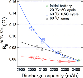
Figure 4. Scatter plot of the capacities and RE 20 °C,50% values of LIBs used to construct the prediction model.
Download figure:
Standard image High-resolution imagePrediction of LIB Discharge Capacity and Internal Resistance Via Machine Learning
We constructed a prediction model for LIB capacity via machine learning using the random forest approach
26,27
in R statistical computing software.
28
We evaluated the generalization performance of the model using a 10-fold cross-validation (CV). Here, an ntree (the number of trees) of 10,000 and mtry (the number of variable par level) of 8, as hyperparameters, were optimized to achieve the lowest root mean squared error for the predictions with respect to the actual values, RMSECV
, in the test data. In addition, RMSECV
indicates the average value for the 10-fold cross-validation, where a low RMSECV
indicates an accurate prediction of the generic data. The coefficient of determination between the predicted and experimental values,  was also calculated for reference, where a high
  indicates an accurate prediction. The random forest approach was used to estimate the remaining useful life
29
or impedance of LIBs.
30
indicates an accurate prediction. The random forest approach was used to estimate the remaining useful life
29
or impedance of LIBs.
30
We carefully selected the impedance measurement frequencies to achieve fast capacity prediction with high precision. The details of the selection are explained later. Figure 5a and 5b shows Bode plots measured from 10–2 Hz to 105 Hz with 12 points per decade (full impedance), measured at 10–1, 100, 101, 102, and 103 Hz (selected impedance). Figures 5c and 5d also shows the RMSECV of the predicted capacity and measurement time for each condition in the impedance measurements, respectively. The capacity was predicted using the temperature and OCV, as well as the real and imaginary parts of the impedance (Z' and Z'', respectively) as explanatory variables. As the impedance depends on the SOC and temperature, information on the SOC, temperature, and impedance should be added to the explanatory variables for predictions at temperatures from −20 °C to 50 °C and SOCs from 0% to 100%. However, the SOC could not be obtained unless the capacity was measured; thus, we used the OCV as one of the explanatory variables, which can be measured over a short period and has a strong correlation with the SOC.

Figure 5. Bode diagrams of the impedance measured from (a) 10–2 Hz to 105 Hz with 12 points per decade and (b) at 10–1, 100, 101, 102, and 103 Hz. (c) RMSECV of the predicted discharge capacity using all 85 impedance points and the five selected impedance points. (d) Measurement time for all 85 impedance points and the five selected impedance points.
Download figure:
Standard image High-resolution imageThe RMSECV
using the selected impedance was lower than that obtained using the full impedance (Fig. 5c). The measurement time for the selected frequencies was also significantly shorter than that for the full impedance (Fig. 5d). Here, we discuss why the above-mentioned selected impedance values are preferable for the diagnosis. Table I lists the RMSECV
,  and measurement time evaluated under each impedance measurement condition. The results indicate that an appropriate frequency region exists for capacity prediction. Impedance at 104–105 Hz had negative effects on the prediction because the individual difference in impedance at 104–105 Hz is larger than the change in impedance with capacity fading. Furthermore, the dispersion of impedances obtained at 105 Hz for the initial LIBs at 20 °C and an SOC of 50% was 2.0 × 10⁻³ Ω2, which was one order of magnitude larger than the 2.3 × 10⁻⁴ Ω2 obtained at 103 Hz. The accuracy of the prediction did not decrease by partially thinning the impedance measurement points. As a result, the RMSECV
using impedances measured at 10–2, 10–1, 100, 101, 102, and 103 Hz was the lowest among all considered cases. However, measuring the impedance required approximately "1/frequency" seconds per point; therefore, the impedance measurement time at 10–2 Hz was approximately 100 s. To satisfy the fast measurement requirements and obtain high-precision predictions, the impedance at 10–2 Hz should be removed from the explanatory variables for the prediction. The measurement time could be reduced to 47 s by skipping the impedance measurements at 10–2 Hz. The RMSECV
without impedance at 10–2 Hz was comparable to that with impedance at 10–2 Hz. Therefore, using the impedances at 10–1, 100, 101, 102, and 103 Hz is optimal for fast predictions with high precision. As a side note, the prediction accuracy of capacity may be heightened by including a specific impedance point as well as 10–2 Hz in the explanatory variables.
and measurement time evaluated under each impedance measurement condition. The results indicate that an appropriate frequency region exists for capacity prediction. Impedance at 104–105 Hz had negative effects on the prediction because the individual difference in impedance at 104–105 Hz is larger than the change in impedance with capacity fading. Furthermore, the dispersion of impedances obtained at 105 Hz for the initial LIBs at 20 °C and an SOC of 50% was 2.0 × 10⁻³ Ω2, which was one order of magnitude larger than the 2.3 × 10⁻⁴ Ω2 obtained at 103 Hz. The accuracy of the prediction did not decrease by partially thinning the impedance measurement points. As a result, the RMSECV
using impedances measured at 10–2, 10–1, 100, 101, 102, and 103 Hz was the lowest among all considered cases. However, measuring the impedance required approximately "1/frequency" seconds per point; therefore, the impedance measurement time at 10–2 Hz was approximately 100 s. To satisfy the fast measurement requirements and obtain high-precision predictions, the impedance at 10–2 Hz should be removed from the explanatory variables for the prediction. The measurement time could be reduced to 47 s by skipping the impedance measurements at 10–2 Hz. The RMSECV
without impedance at 10–2 Hz was comparable to that with impedance at 10–2 Hz. Therefore, using the impedances at 10–1, 100, 101, 102, and 103 Hz is optimal for fast predictions with high precision. As a side note, the prediction accuracy of capacity may be heightened by including a specific impedance point as well as 10–2 Hz in the explanatory variables.
Table I.
RMSECV
,  and measurement time evaluated under each condition during impedance measurements.
| Impedance frequency (Hz) | RMSECV (mAh) |

| Measurement time(s) |
|---|---|---|---|
| 10−2 to 105 (85 points) | 53.67 | 0.883 | 1,170 |
| 10−2, 10−1, 100, 101, 102, 103, 104, 105 | 53.24 | 0.882 | 199 |
| 10−2, 10−1, 100, 101, 102, 103, 104 | 47.63 | 0.906 | 194 |
| 10−2, 10−1, 100, 101, 102, 103 | 43.60 | 0.919 | 189 |
| 10−2, 10−1, 100, 101, 102 | 47.96 | 0.900 | 184 |
| 10−1, 100, 101, 102, 103 | 44.01 | 0.916 | 47 |
| 100, 101, 102, 103 | 44.55 | 0.915 | 33 |
| 103 | 58.78 | 0.848 | 15 |
Figure 6a shows a scatter plot of the predicted values and measured capacities for predictions using the temperature, OCV, and impedances at 10–1, 100, 101, 102, and 103 Hz as the explanatory variables. Figure 6a also shows the borderlines within which 90% of the data were contained. We then constructed a prediction model in which 90% of the data were contained within an error of ± 29 mAh for a capacity of 2,987–3,432 mAh. The RMSECV
and  were 44.01 mAh and 0.916, respectively. Knowledge of the degradation of internal resistance is important when assessing whether to reuse or recycle LIBs. Therefore, we predicted RE
20 °C,50% as an index of internal resistance degradation, using the same explanatory variable as that for capacity prediction. Figure 6b shows a scatter plot of the predicted values and the measured RE
20 °C,50%. Ninety percent of the data were contained in the prediction model within an error of ± 0.0016 Ω for RE
20 °C,50% at 0.0569–0.113 Ω. The RMSECV
and
were 44.01 mAh and 0.916, respectively. Knowledge of the degradation of internal resistance is important when assessing whether to reuse or recycle LIBs. Therefore, we predicted RE
20 °C,50% as an index of internal resistance degradation, using the same explanatory variable as that for capacity prediction. Figure 6b shows a scatter plot of the predicted values and the measured RE
20 °C,50%. Ninety percent of the data were contained in the prediction model within an error of ± 0.0016 Ω for RE
20 °C,50% at 0.0569–0.113 Ω. The RMSECV
and  were 0.0033 Ω and 0.961, respectively. It is thought that RE
20 °C,50% is easy to predict because RE
20 °C,50% is obtained by impedance. However, the temperature and SOC for the diagnosis are not always 20 °C and 50%, respectively; thus, predicting RE
20 °C,50% is not simple. Consequently, the capacity and internal resistance can be simultaneously predicted with high precision within 1 min Hereafter, we used the temperature, OCV, and impedances at 10–1, 100, 101, 102, and 103 Hz as explanatory variables for prediction of the capacity and RE
20 °C,50%.
were 0.0033 Ω and 0.961, respectively. It is thought that RE
20 °C,50% is easy to predict because RE
20 °C,50% is obtained by impedance. However, the temperature and SOC for the diagnosis are not always 20 °C and 50%, respectively; thus, predicting RE
20 °C,50% is not simple. Consequently, the capacity and internal resistance can be simultaneously predicted with high precision within 1 min Hereafter, we used the temperature, OCV, and impedances at 10–1, 100, 101, 102, and 103 Hz as explanatory variables for prediction of the capacity and RE
20 °C,50%.
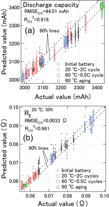
Figure 6. Scatter plot of predicted and measured (a) discharge capacities and (b) RE 20 °C,50% values using the temperature, open-circuit voltage (OCV), and impedances at 10–1, 100, 101, 102, and 103 Hz as the explanatory variables. Parts (a) and (b) show the borderlines within which 90% of the data were contained.
Download figure:
Standard image High-resolution imageValidation of Prediction Model Generalization Performance
To validate the generalization performance of the prediction model, we prepared additional degraded LIBs using different deterioration test conditions. LIBs were tested via repeated charges of 1 C or 2.5 C, followed by discharges of 0.1 C between 2.5 V and 4.2 V at 20 °C (20 °C-1C cycle or 20 °C-2.5 C cycle). We also prepared LIBs degraded via 60 °C-0.5C-450 cycles to validate the prediction accuracy of the constructed prediction model in the extrapolation area. Table S2 in the supplementary material lists the capacities and RE 20 °C,50% values of the additional degraded LIBs. Furthermore, we prepared complex-degraded LIBs to validate the prediction accuracy of the prediction model, for example, one LIB was degraded through a 20 °C-2C cycle, followed by 60 °C-aging or a 60 °C-0.5 C cycle. Table II lists the capacities and RE 20 °C,50% values of the complex-degraded LIBs. Figure 7 shows a scatter plot of the capacities and RE 20 °C,50% of the additional degraded LIBs and complex-degraded LIBs.
Table II. Degradation process, discharge capacity, RE 20 °C,50%, absolute error of predicted value with respect to the measured capacity (ΔQ), and RE 20 °C,50% (ΔRE 20 °C,50%) for each complex-degraded LIB.
| Battery ID | Battery state | Capacity(mAh) | RE 20 °C,50% (Ω) | ΔQ(mAh) | ΔRE 20 °C,50% (Ω) |
|---|---|---|---|---|---|
| A-1 | 60 °C-20 days → 20 °C-2C-21 cycles | 3,280 → 2,887 | 0.0644 → 0.0688 | 238 | 0.0007 |
| A-2 | 60 °C-215 days → 20 °C-2C-30 cycles | 3,051 → 3,069 | 0.0789 → 0.0879 | 14 | 0.0060 |
| B-1 | 60 °C-0.5C-80 cycles → 20 °C-2C-30 cycles | 3,233 → 3,070 | 0.0713 → 0.0776 | 68 | 0.0013 |
| B-2 | 60 °C-0.5C-325 cycles → 20 °C-2C-30 cycles | 2,987 → 3,005 | 0.114 → 0.123 | 16 | 0.0164 |
| C-1 | 60 °C-0.5C-80 cycles → 60 °C-47 days | 3,226 → 3,144 | 0.0715 → 0.0798 | 10 | 0.0017 |
| C-2 | 60 °C-0.5C-325 cycles → 60 °C-47 days | 2,990 → 2,950 | 0.113 → 0.129 | 81 | 0.0272 |
| D-1 | 20 °C-2C-9 cycles → 60 °C-47 days | 3,254 → 3,191 | 0.0560 → 0.0752 | 66 | 0.0059 |
| D-2 | 20 °C-2C-60 cycles → 60 °C-47 days | 3,007 → 3,004 | 0.0624 → 0.0866 | 72 | 0.0078 |
| E-1 | 20 °C-2C-12 cycles → 60 °C-0.5C-80 cycles | 3,237 → 3,119 | 0.0553 → 0.0743 | 43 | 0.0020 |
| E-2 | 20 °C-2C-63 cycles → 60 °C-0.5C-80 cycles | 3,054 → 2,952 | 0.0633 → 0.0820 | 194 | 0.0082 |

Figure 7. Scatter plot of capacities and RE 20 °C,50% values of the LIBs used to evaluate the prediction model. The arrows indicate changes that occurred as a result of degradation between the first and second process.
Download figure:
Standard image High-resolution imageThe data for LIBs degraded via the 20 °C cycle were plotted on the curve shown in Fig. 7, regardless of the C-rate from 1 C to 2.5 C. Therefore, we confirmed the accuracy of the prediction model using two LIBs degraded through a 20 °C-1C cycle and two LIBs degraded through a 20 °C-2.5 C cycle, for which the actual capacity was 3,170–3,217 mAh. Figure 8a shows a contour plot of the average capacity prediction error with respect to the measured capacity values of the four LIBs at each temperature and SOC, ranging from −20 °C to 50 °C and 0%–100%, respectively. Most of the capacity prediction error for the four LIBs in the full range of temperatures and SOCs (Fig. 8a) was comparable to an RMSECV of 44.01 mAh for the constructed prediction model. In particular, high-precision prediction occurred at approximately 0 °C. The reason for this is not clear but is currently under consideration. The difference in the C-rate slightly affected the capacity prediction error under the degraded condition, that is, a C-rate from 1 C to 2.5 C at 20 °C, because the prediction error for the 20 °C-2.5 C cycle LIBs was similar to that of the 20 °C-1C cycle LIBs. Figure 8b shows a contour plot of the average RE 20 °C,50% prediction error with respect to the measured values of the four LIBs at each temperature and SOC, ranging from −20 °C to 50 °C and 0%–100%, respectively. The overall prediction error for RE 20 °C,50% was small. Moreover, high-precision prediction was achieved at approximately 0 °C. The difference in the C-rate from 1 C to 2.5 C slightly affected the prediction error for RE 20 °C,50%, which was identical to the results of the capacity prediction.
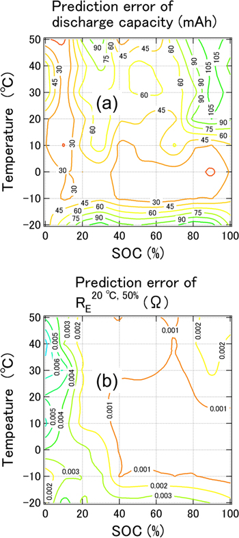
Figure 8. Contour plots of the average prediction error for (a) capacity and (b) RE 20 °C,50% with respect to the measured value of LIBs. Two LIBs were degraded through the 20 °C-1C cycle and two LIBs were degraded through the 20 °C-2.5 C cycle, in which the capacity was approximately 3,200 mAh.
Download figure:
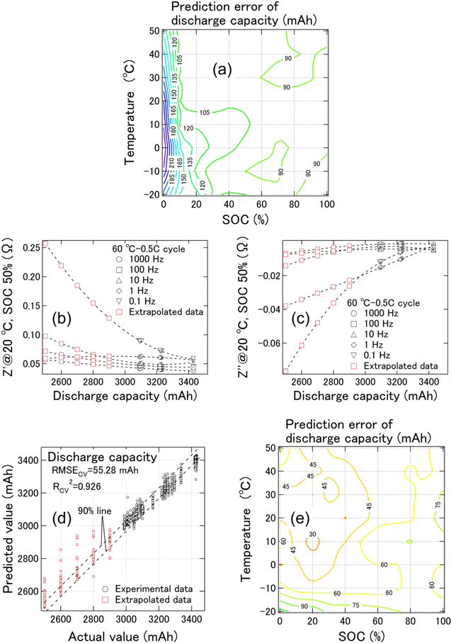
Standard image High-resolution imageAlthough predicting a value in an extrapolation area is usually difficult, we were able to confirm the prediction accuracy of the constructed prediction model in the extrapolation area. We prepared the LIBs degraded by the 60°C-0.5C-450 cycle, which lay in the extrapolation area of the data set (80–325 cycles) used for the prediction model. Figure 9a shows a contour plot of the average capacity prediction error with respect to the measured value of the two LIBs degraded through the 60 °C-0.5C-450 cycle (Table SII). Under conditions of −20 °C to 50 °C and SOCs from 0% to 100%, the predicted capacities of the LIBs degraded through the 60 °C-0.5C-450 cycle were ≥90 mAh higher than the actual values of approximately 2,910 mAh, although the prediction model was constructed with an RMSECV of 44.01 mAh. This yielded a lower limit for the predicted capacity, which was restricted by actual values of approximately 3,000 mAh for LIBs degraded through the 60 °C-0.5C-325 cycle.
Figure 9. (a) Contour plot of the average prediction error for discharge capacity with respect to the measured value of two LIBs degraded through the 60 °C-0.5C-450 cycle. (b) and (c) Discharge capacity dependence of Z' and Z'' respectively, at 20 °C and an SOC of 50% for LIBs degraded through the 60 °C-0.5 C cycle at each frequency. The red squares denote data extrapolated from the measured values at each frequency. (d) Scatter plot of the predicted values and measured capacities when extrapolated data were added to the dataset to construct the prediction model. Part (d) shows the borderlines within which 90% of the data were contained. (e) Contour plot of the average prediction error for discharge capacity with respect to the measured value of two LIBs degraded through the 60 °C-0.5C-450 cycle with the addition of extrapolated data.
Download figure:
Standard image High-resolution image
Therefore, we reconstructed the capacity prediction model by adding data extrapolated from the measured impedances to the dataset above. The extrapolated curve was defined as y = ax2 + bx + c (y: Z' or Z''; x: capacity), with the addition of extrapolated data at 2,500, 2,600, 2,700, 2,800, and 2,900 mAh. Figures 9b and 9c shows the capacity dependence of Z' and Z'' at 20 °C and an SOC of 50% for the 60 °C-0.5 C cycle LIBs at each frequency. Incidentally, the capacities from our data could not be fitted perfectly using a linear regression of the impedance, as was the case in a previous study. 6 Data denoted by the red squares in Figs. 9b and 9c indicate the added data at a temperature and SOC of 20 °C and 50%, respectively. Figure 9d shows a scatter plot of the predicted values and measured capacities when extrapolated data were added to the dataset to construct the prediction model. Figure 9d also shows the borderlines, which contain 90% of the data. The prediction accuracy for capacity was slightly affected by additional extrapolated data. Figure 9e shows a contour plot of the average prediction error for capacity with respect to the measured value of two LIBs degraded through the 60 °C-0.5C-450 cycle with the addition of the extrapolated data. The prediction accuracy improved significantly from Figs. 9a to 9e by using the reconstructed model with the addition of extrapolated data. An extrapolated area always exists unless degraded LIBs with a capacity of 0 mAh are prepared. Therefore, to the greatest extent possible, extrapolated data should be added to the dataset during construction of the prediction model to improve the generalization performance. However, we note that the choice of an extrapolated curve is important for improving the prediction, although y = ax2 + bx + c was used for the extrapolated curve in this study.
As LIBs that have been degraded through multiple processes are generally more common in LIB markets than those degraded through only one process, we validated the prediction accuracy of the prediction model using data from complex-degraded LIBs. The arrows for the complex-degraded LIBs in Fig. 7 indicate the changes that occurred between the first and the second degradation process. The change in capacity and RE 20 °C,50% of batteries B-1 or E-1 can be explained by a simple combination of the 20 °C-2C cycle and 60 °C-0.5 C cycle. The change in capacity and RE 20 °C,50% of battery A-1 can also be explained by a simple combination of 60 °C-aging and the 20 °C-2C cycle. In contrast, the change in capacity and RE 20 °C,50% of batteries C-1 and D-1 cannot be explained by a simple combination of the first and second processes. In batteries A-2 and B-2, the capacity did not decrease as a result of the second degradation because the total quantity of the 2 C charge was low owing to the high resistance of the LIBs after the first degradation. As mentioned above, a variety of degraded LIBs can be prepared to validate the generalization performance of the constructed prediction model.
Table II lists the prediction error for the measured capacity (ΔQ) and RE 20 °C,50% (ΔRE 20 °C,50%) of each complex-degraded LIB using impedances at 20 °C and an SOC of 50%. Most of the error in the complex-degraded LIBs was comparable to an RMSECV of 44.01 mAh for the constructed prediction model. The prediction accuracy for each complex-degraded LIB in Table II was comparable to that at any condition from −20 °C to 50 °C and SOCs from 0% to 100%. Comparatively, the error for battery C-2 was slightly large due to its location in the extrapolation area; however, the error could be reduced to 19 mAh from 81 mAh using the above-mentioned reconstructed prediction model with the addition of extrapolated data. The errors for batteries A-1 and E-2 were significantly larger than those for the other complex-degraded LIBs. One of the reasons is that these batteries were also located in the extrapolation area. The error for batteries A-1 and E-2 could be reduced to 172 mAh and 141 mAh, respectively, when the capacity prediction model was reconstructed with additional data extrapolated from the measured impedances of 20 °C-2C cycle LIBs, 60 °C-aged LIBs, and 60 °C-0.5 C cycle LIBs (the extrapolated curve was defined as y = ax2 + bx + c). However, as the errors remained large even when extrapolated data were added to the dataset, the complex degradation effect cannot be ignored in severely degraded LIBs. To accurately predict the resistances of complex-degraded LIBs, the impedance data of these LIBs should be added to the data set for the prediction model in advance. Otherwise, impedance data for complex-degraded LIBs are created as a simple combination of the degradation processes used for model construction. Furthermore, regarding the RE 20 °C,50% of the complex-degraded LIBs, with the exception of B-2 and C-2, which lay within the extrapolation area, all values were comparable to an RMSECV of 0.0033 Ω for the constructed prediction model.
We show the simultaneous prediction of the capacity and typical resistance of NCA/graphite LIBs with high accuracy in a short period of time. This diagnostic method using selected impedances is probably applicable to LIBs with a graphite anode and a Li(Ni,Mn,Co)O2 (NMC) cathode 6,8,9,17 because main degradation causes of the LIBs are the same as those of NCA/graphite LIBs (SEI growth at the anode, Li plating at the anode, electrode material cracking and decomposition at the cathode). However, the correlation between capacity and impedance of LiCoO2 (LCO)/graphite 7 or LiFePO4 (LFP)/graphite 2,16,18 LIBs may be a little bit different from that of NCA/graphite LIBs because the contribution of the transition metal dissolution to capacity fade cannot be ignored in LCO/graphite or LFP/graphite LIBs. Note that a dataset for prediction should be prepared in each battery type as the capacities and impedances depends on battery types. The diagnosis for the LIBs as mentioned above will be validated in future work and the diagnostic method using selected impedances will be applied to various batteries such as lithium-sulfur batteries 20,31 and sodium-sulfur batteries. 32
Conclusions
To develop a nondestructive and rapid method of diagnosing degradation in used LIBs with high precision at any temperature or SOC, we attempted to simultaneously predict the capacity and internal resistance via machine learning using the impedance, temperature, and OCV. First, we prepared three types of degraded LIBs using 18650-type cylindrical LIBs, then developed a dataset by measuring the discharge capacity at 0.1 C as well as the impedance and OCV at each temperature and SOC, which ranged from −20 °C to 50 °C and 0%–100%, respectively. To evaluate degradation of the internal resistance, a typical internal resistance (RE 20 °C,50%) was defined using the impedance at 20 °C and an SOC of 50%. Second, we trained the capacity or RE 20 °C,50% using impedance, temperature, and OCV via machine learning. Using the OCV, temperature, and impedances at 10−1, 100, 101, 102, and 103 Hz as explanatory variables, we constructed a prediction model in which 90% of the data lay within an error of ±25 mAh for a discharge capacity of 2,987–3,432 mAh for all three types of degraded LIBs. The prediction model was able to estimate the capacity after less than 1 min of impedance measurement. Furthermore, the RE 20 °C,50% could be predicted with high precision using the same explanatory variables. Third, we prepared different types of degraded LIBs and validated the generalization performance of the prediction model. This model can be applied in most cases, but is inappropriate for LIB data in the extrapolation area. To solve this problem, extrapolated curves were created using the obtained data; the resulting data can be added to the dataset to reconstruct the prediction model. The practical diagnostic method proposed in this study promotes the reuse of used LIBs and greatly contributes to constructing a battery circulation economy.
Acknowledgments
We would like to thank Dr. Sasaki at Toyota Central R&D Laboratories for valuable discussions, and Dr. Nozaki at Toyota Central R&D Laboratories for sample preparation support. We would also like to thank Editage (www.editage.com) for English language editing. This research did not receive any specific grant from funding agencies in the public, commercial, or not-for-profit sectors.