Abstract
The maximum energy that lithium-ion batteries can store decreases as they are used because of various irreversible degradation mechanisms. Many models of degradation have been proposed in the literature, sometimes with a small experimental data set for validation. However, a comprehensive comparison between different model predictions is lacking, making it difficult to select modelling approaches which can explain the degradation trends actually observed from data. Here, various degradation models from literature are implemented within a single particle model framework and their behavior is compared. It is shown that many different models can be fitted to a small experimental data set. The interactions between different models are simulated, showing how some of the models accelerate degradation in other models, altering the overall degradation trend. The effects of operating conditions on the various degradation models is simulated. This identifies which models are enhanced by which operating conditions and might therefore explain specific degradation trends observed in data. Finally, it is shown how a combination of different models is needed to capture different degradation trends observed in a large experimental data set. Vice versa, only a large data set enables to properly select the models which best explain the observed degradation.
Export citation and abstract BibTeX RIS

This is an open access article distributed under the terms of the Creative Commons Attribution 4.0 License (CC BY, http://creativecommons.org/licenses/by/4.0/), which permits unrestricted reuse of the work in any medium, provided the original work is properly cited.
The amount of energy that a lithium-ion (Li-ion) battery can store decreases over its lifetime. This is the result of various mechanical and electrochemical processes, many of which are influenced by operating conditions. In order to predict the lifetime of a battery and the sensitivity of degradation to different load profiles, many models of degradation have been proposed. These can broadly be divided into three categories:
First, empirical models, i.e. parametric functions interpolating a data set from a large scale cycling experiment. These can be very effective, but lack generality because they are only valid for the exact battery chemistry and operating conditions tested in the experiment, and they may exhibit growing inaccuracy of battery health predictions when used for long range extrapolation.1–5
A second class are physical models. These are typically collections of partial differential equations describing the physical processes taking place in a battery. They are useful for gaining insight into possible degradation mechanisms, and could be more robust than pure empirical approaches, but often are computationally complex, and have many parameters which may be unknown.3,6–9
Finally, a more recent development are 'machine learning' models. These are typically black box approaches, similar to the empirical approach, but with greater flexibility. They can be fast and accurate, but require a large data set to be effective, and it is often difficult to interpret and explain their outcomes.10–14
To investigate the mechanisms of battery aging, physical models are interesting because they offer a set of testable hypotheses about the underlying reasons for degradation. However, because of the multitude of processes taking place, and the complexity of each, simplifications have to be made, for example by ignoring certain processes, in order to have a computationally tractable approach.
For a single mechanism, i.e. a physical process that causes battery degradation, multiple models, i.e. sets of mathematical equations, have been proposed in the literature. Table I gives an overview of the different models that have been proposed. Fig. 1 represents the various models graphically. Most studies only consider a limited number of models describing a few mechanisms. This paper gives a comprehensive overview of the wide range of existing models including specific case studies as examples. They have been implemented here within a flexible modelling approach which allows one to assess their individual effects and interactions. Finally, the impact of variable operating conditions on degradation according to the different approaches is investigated, and also, the fitting of a large experimental data set using a combination of models and mechanisms is demonstrated.
Table I. Overview of various degradation models grouped by physical degradation mechanism.
| SEI growth | Crack growth | LAM | |||||||||||
|---|---|---|---|---|---|---|---|---|---|---|---|---|---|
| kinetically | solvent | electron | simplified | physical | physical | simplified | physical | physical | simplified | Li-plating | |||
| Paper | limited | diffusion limited | tunneling | correlation | stress | crack growth | correlation | stress | crack growth | correlation | dissolution | kinetic | other |
| Appiah, 201616 | x | x | x | ||||||||||
| Ashwin, 201617 | x | ||||||||||||
| Barai, 201518 | x | ||||||||||||
| Cannarella, 201519 | x | ||||||||||||
| Christensen, 200520 | x | x | x | ||||||||||
| Delacourt, 201221 | x | x | |||||||||||
| Deshpande, 201222 | x | x | x | ||||||||||
| Deshpande, 201723 | x | x | |||||||||||
| Ekstrom, 201524 | x | x | x | ||||||||||
| Ge, 201725 | x | ||||||||||||
| Jin, 201726 | x | x | x | ||||||||||
| Kamyab, 201927 | x | x | |||||||||||
| Kindermann, 2017 28 | x | x | x | ||||||||||
| Kupper, 201729 | x | x | |||||||||||
| Kupper, 201830 | x | x | x | x | x | ||||||||
| Laresgoiti, 2015 31 | x | x | x | ||||||||||
| Legrand, 201432 | x | ||||||||||||
| Li, 201533 | x | ||||||||||||
| Lin, 201334 | x | x | x | x | |||||||||
| Narayanrao, 201235 | x | x | x | ||||||||||
| Ning, 200436 | x | ||||||||||||
| Pinson, 201337 | x | x | |||||||||||
| Ploehn, 200438 | x | ||||||||||||
| Purewal, 201439 | x | x | x | ||||||||||
| Ramadass, 200440 | x | ||||||||||||
| Randall, 201241 | x | ||||||||||||
| Sarafi, 2009 42 | x | x | |||||||||||
| Safari, 201043 | x | x | |||||||||||
| Safari, 201144 | x | x | |||||||||||
| Single, 201745 | x | x | |||||||||||
| Tahmasbi, 201746 | x | x | |||||||||||
| Tang, 201247 | x | x | x | ||||||||||
| Yang, 201748 | x | x | x | ||||||||||
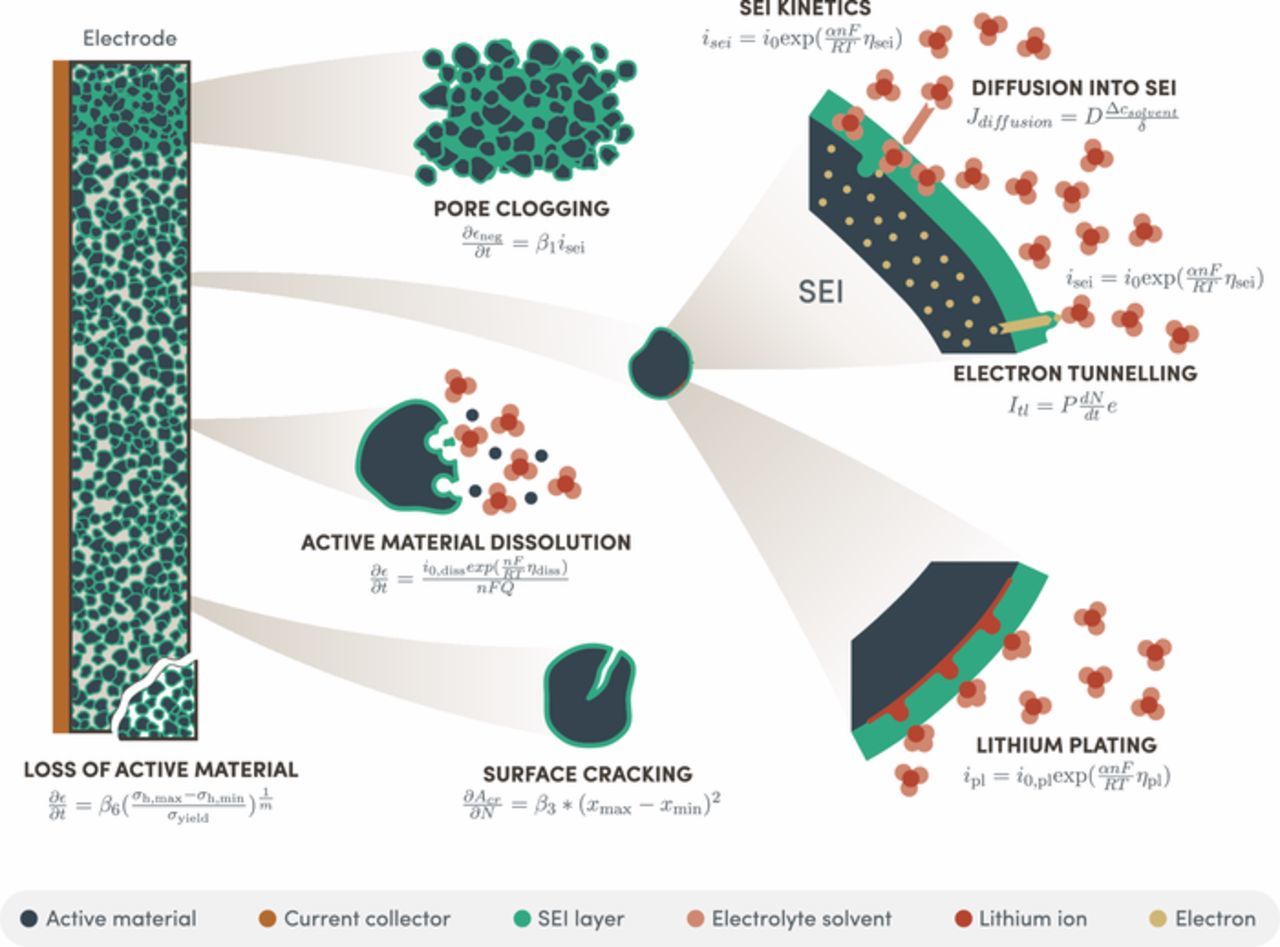
Figure 1. Graphical illustration of the various degradation mechanisms with typical equations modelling each mechanism.
The focus of this paper is on lithium-ion chemistries with graphite negative electrodes. An open-access version of the code used to simulate the results in this paper is available on GitHub.15
Methods
Battery model
Physical degradation models depend on the underlying physical states, such as the lithium concentration at various points in the battery. Therefore, a model is needed in order to calculate these states starting from an initial condition and assuming a given load profile. Various physical battery models exist, at different length scales, offering differing amounts of detail and computational complexity. Material properties can be simulated using ab initio calculations, e.g. Persson et al.49 used kinetic Monte Carlo simulations to calculate the diffusion coefficient of lithium in graphite, while von Wald et al.50 used a combination of density functional theory and molecular dynamics to study the effect of the SEI layer on lithium intercalation. Phase changes in particles are typically studied using phase-field approaches, such as Bai et al.51 who simulated phase separation in LFP particles. On a higher level, the microstructure of porous electrodes can be simulated using non-equilibrium thermodynamics, for instance Latz et al.52 used the software BEST for virtual electrode design.
Continuum models have often been used for degradation simulations because they take significantly less computational power and time in comparison to ab initio simulations, but this comes at the cost of having to assume more homogeneous cell behavior. Kupper et al.29,30 used a '1D+1D+1D multi-scale model' for degradation simulations allowing them to incorporate detailed chemical reactions and multi-phase chemistry. However, they had to use a time-upscaling methodology to accelerate the simulations, and even then, simulating one full cycle still took about 1 minute of computational time. One of the most popular models for degradation simulations is based upon the so-called 'pseudo-2D' (P2D) model, originally developed by the Newman group53 and based on porous electrode theory, which simulates lithium transport and diffusion in two dimensions, by placing spherical particles along the thickness of the cell, allowing a concentration gradient over the thickness of an electrode depending on the electrolyte transport. This is important for simulating lithium plating, which typically occurs in the region close to the separator.48 Due to its algebraic constraints, the P2D model takes a significant amount of computational power and time to solve, which was deemed prohibitive here due to the large number of simulations required for this review.
The simplest continuum model is the single particle model (SPM), which is an order of magnitude faster to compute. It removes the 'thickness' dimension from the P2D model such that only one spherical particle is simulated for each electrode while the electrolyte is ignored all together. It also cannot simulate inhomogeneities and other local effects, for which more complex battery models are needed. Although inhomogeneities can be important for degradation54–56 the SPM was chosen to keep the computational time manageable whilst still capturing the average degradation of an entire cell.
In this study, a negative current means the battery is charging, while a positive current discharges the battery. The terms anode and negative electrode are used interchangeably in this paper, in the usual fashion. Whilst this is correct for discharging, strictly speaking during charging the anode is the positive electrode and the cathode is the negative electrode. The time dependency of most variables has been omitted in the equations for simplicity.
The SPM is a basic 'averaged' electrochemical model of a lithium-ion battery where only solid state diffusion transport and spatially uniform kinetics are accounted for .36,40,57–59 Each electrode is represented by a sphere. In the sphere, the time-dependent molar lithium concentration ci(r, t) in  is calculated as a function of radius r, where subscript i ∈ { −, +} refers to the negative or positive electrode respectively. Fick's law of diffusion relates the time derivative to the gradient and the diffusion constant Di,
![Equation ([1])](https://content.cld.iop.org/journals/1945-7111/166/14/A3189/revision1/d0001.gif)
At the center of the sphere, the gradient has to be zero due to symmetry, while at the surfaces, the gradient is equal to the molar flux ji, which is related to the current density on that electrode ii via Faraday's constant F and the number of electrons participating in the reaction, n. Thus the boundary conditions are
![Equation ([2])](https://content.cld.iop.org/journals/1945-7111/166/14/A3189/revision1/d0002.gif)
![Equation ([3])](https://content.cld.iop.org/journals/1945-7111/166/14/A3189/revision1/d0003.gif)
The product of the electrode volume Vi and the effective electrode surface area ai relates the current density to the total battery current I. The specific surface area is a function of the radius of the particle Ri and the volume fraction of active material  i36 according to
![Equation ([4])](https://content.cld.iop.org/journals/1945-7111/166/14/A3189/revision1/d0004.gif)
The main intercalation reaction happens at the surface of each sphere, and is assumed to follow Butler-Volmer kinetics with a rate constant ki, a constant lithium concentration in the electrolyte cel, a transfer coefficient α, the maximum lithium concentration  , and the ideal gas constant R, such that the current density ii can be calculated from the overpotential ηi at a battery temperature T36 according to
![Equation ([5])](https://content.cld.iop.org/journals/1945-7111/166/14/A3189/revision1/d0005.gif)
![Equation ([6])](https://content.cld.iop.org/journals/1945-7111/166/14/A3189/revision1/d0006.gif)
Because temperature is a key determinant of the battery degradation rate, a lumped thermal model was added to the SPM.60 There are three heat sources, viz. ohmic heating due to the DC resistance of the battery  , reaction heating due to the overpotentials, and entropic heating as given by the entropic coefficient
  . Convective heat transfer to the environment at a temperature of
  with a constant heat transfer coefficient h over a battery surface
  cools the battery, which has a heat capacity of cp, a density ρ, and a cell volume v. Thus,
![Equation ([7])](https://content.cld.iop.org/journals/1945-7111/166/14/A3189/revision1/d0007.gif)
Arrhenius relations with activation energies ED, i and Ek, i are used to calculate the temperature dependency of the diffusion and rate parameters starting from the reference values  and
and  at a reference temperature
  , according to
![Equation ([8])](https://content.cld.iop.org/journals/1945-7111/166/14/A3189/revision1/d0008.gif)
![Equation ([9])](https://content.cld.iop.org/journals/1945-7111/166/14/A3189/revision1/d0009.gif)
Growth of the SEI layer and loss of lithium
Many researchers have argued that the most important lithium-ion battery degradation mechanism is the growth of a passivation layer on the graphite electrode. Components of the electrolyte solvent are reduced at the graphite surface in a reaction with lithium-ions and electrons from the electrode. The reaction products deposit on the graphite forming the solid electrolyte interphase (SEI) layer.61–63 Various reactions have been suggested to occur (depending on the local voltage),64,65 but the reaction modeled by most researchers is one between ethylene carbonate and lithium ions,29,36
![Equation ([10])](https://content.cld.iop.org/journals/1945-7111/166/14/A3189/revision1/d0010.gif)
Horstmann et al.66 and Single et al.67 give an overview of multi-scale models for SEI growth. For the continuum scale that is studied in this work, two models have been suggested for this process. Das et al.68 propose a detailed kinetically limited SEI growth model with spatially resolved concentrations, but most authors36,40 use a kinetically limited SEI growth model using a Tafel equation, with the exchange current density  as a fitting constant. The overpotential for the SEI side reaction
  is a function of the anode potential
  , the anode overpotential
  , the equilibrium potential of the SEI growth reaction
  , and the resistive voltage drop across the existing SEI layer of thickness δ and specific resistance
  :
:
![Equation ([11])](https://content.cld.iop.org/journals/1945-7111/166/14/A3189/revision1/d0011.gif)
![Equation ([12])](https://content.cld.iop.org/journals/1945-7111/166/14/A3189/revision1/d0012.gif)
Alternatively, others have suggested a model which includes the limitation caused by diffusion of the electrolyte through the passivation layer.20,24,27,37,45,46,48 By assuming a constant bulk concentration of solvent  and linear diffusion across the existing SEI layer with a diffusion constant
  , the concentration at the reaction surface can be calculated. This equation can be substituted into the equation for the exchange current density
  , where
  is the rate constant and
  is the solvent concentration at the particle surface. This results in Equation 13 for the SEI side current density, which has one term in the denominator for the reaction kinetics and one for the solvent diffusion. If diffusion is considered to be the rate limiting step, these models predict the typical square root dependency that is often, but not always, seen in the capacity fade over time. If the reaction kinetics is the rate limiting step, the model is very similar to the kinetically limited case. Between those extreme cases, there is a situation where both diffusion and kinetics matter in a similar magnitude.
![Equation ([13])](https://content.cld.iop.org/journals/1945-7111/166/14/A3189/revision1/d0013.gif)
The SEI side reaction and resulting passivation layer growth can have various effects on the battery. First of all, the growth rate of the SEI layer increases linearly with the SEI side current density Ref. 36 according to
![Equation ([14])](https://content.cld.iop.org/journals/1945-7111/166/14/A3189/revision1/d0014.gif)
where M is the molecular weight of the SEI layer and ρ is its density. Secondly, the side reaction consumes Li-ions which can no longer participate in the main reaction (this is termed 'loss of lithium inventory', or LLI). Therefore, the boundary condition for the lithium diffusion at the surface of the graphite has to be changed to include this side reaction.36 The lithium concentration gradient at the negative particle surface becomes a function of the main current density on the negative electrode  and SEI side reaction current density
  according to
![Equation ([15])](https://content.cld.iop.org/journals/1945-7111/166/14/A3189/revision1/d0015.gif)
Thirdly, the SEI layer can block some of the pores of the graphite electrode, resulting in parts of the active material in the electrode no longer being accessible, which increases the current density on the remaining active material. In the single particle model, this can be achieved in an average sense by decreasing the volume fraction of negative active material  , which will increase the current density according to Equations 3 and 4. The equations proposed for pore clogging suggest that the rate at which the volume fraction of negative active material decreases is a linear function of the SEI side reaction current density,17,48 with a fitting constant β1, according to
![Equation ([16])](https://content.cld.iop.org/journals/1945-7111/166/14/A3189/revision1/d0016.gif)
Others have argued that the decrease in porosity should affect the diffusion and rate constants also,45 but this is not included here.
Surface cracking
When Li-ions are intercalated, most electrode materials expand, and they subsequently contract on deintercalation. These volume expansion-contraction cycles lead to alternating stresses in the electrodes, which in turn causes crack propagation and material fatigue. When cracks appear at the surface of the electrode, they increase the surface area on which the SEI layer can grow, leading to more loss of cyclable lithium.
To model this, Laresgoiti et al.31 started with a physical model of the stress and strain in spherical graphite particles and the SEI layer surrounding them, before simplifying it to a correlation between surface concentration and stress. They then used Wöhler curves with slope m1 to relate the number of cycles to failure to the stress variation during a cycle  relative to the maximum yield strength
  . Wöhler curves are the result of statistical analysis of metal fatigue,69 and as such the value of m1 is determined by fitting the simulation to experimental data. The yield strength is a material property but is treated as a fitting parameter due to a lack of experiments to measure it. Assuming a linear damage accumulation, Laresgoiti et al. related the lost charge capacity
  per cycle N to this mean stress with a fitting parameter β2, according to
![Equation ([17])](https://content.cld.iop.org/journals/1945-7111/166/14/A3189/revision1/d0017.gif)
Alternatively, Deshpande et al.23 started from a physical stress model, which they then simplified to a quadratic relation between the increase in crack surface area  and the concentration swing over that cycle, with fitting parameter β3. The concentration swing is the difference between the highest and lowest Li-fractions x during the cycle. The Li-fraction is the lithium concentration relative to the maximum lithium concentration
  . Thus,
![Equation ([18])](https://content.cld.iop.org/journals/1945-7111/166/14/A3189/revision1/d0018.gif)
Others follow a more empirical approach. Barai et al.18 assume that crack growth increases exponentially with charge throughput until it plateaus at a (constant) maximum crack surface area  . This means that the time derivative of the crack surface area is proportional to the existing crack surface area and the absolute value of the current with a fitting constant β4. They argue that these cracks also increase the tortuosity, resulting in a decreasing effective diffusion constant
  with a fitting parameter β5. This can be expressed as
![Equation ([19])](https://content.cld.iop.org/journals/1945-7111/166/14/A3189/revision1/d0019.gif)
![Equation ([20])](https://content.cld.iop.org/journals/1945-7111/166/14/A3189/revision1/d0020.gif)
Ekstrom et al. and Kindermann et al.24,28 assumed that additional SEI growth due to crack growth could be simulated by a second side reaction current which follows a Tafel equation. The difference compared to the original SEI side reaction is that the rate constant of the crack growth reaction  is a function of the Li-fraction
  , to represent the phase transitions in the graphite. Thus the side reaction current is
![Equation ([21])](https://content.cld.iop.org/journals/1945-7111/166/14/A3189/revision1/d0021.gif)
Loss of active material
The previous section was about cracks initiating at electrode surfaces and growing. Similar underlying physical phenomena (such as alternating stresses) can also lead to cracks forming within electrodes. This can cause loss of electrical contact, and a reduction of the usable active material.
Several researchers have developed mechanical stress models for spherical particles of radius R0.70–74 They all arrive at similar equations for the radial stress σr and the tangential stress σt at radius r, where Ω is the partial molar volume, E is the Young's modulus, ν is the Poisson's ratio, c is the Li-concentration as a function of the radius and ζ is a dummy integration variable. The equations for radial and tangential stress, respectively, are
![Equation ([22])](https://content.cld.iop.org/journals/1945-7111/166/14/A3189/revision1/d0022.gif)
![Equation ([23])](https://content.cld.iop.org/journals/1945-7111/166/14/A3189/revision1/d0023.gif)
The radial and tangential stress can be combined into the hydrostatic stress σh, given by
![Equation ([24])](https://content.cld.iop.org/journals/1945-7111/166/14/A3189/revision1/d0024.gif)
These authors did not link this stress to a degradation effect, but the previous section provided many correlations between stress and crack growth. Because the underlying principles are the same, these correlations can also be used to calculate the loss of active material (LAM) in the electrodes. The LAM can be simulated by decreasing the volume fraction of active material according to
![Equation ([25])](https://content.cld.iop.org/journals/1945-7111/166/14/A3189/revision1/d0025.gif)
which is similar to Equation 17. This will increase the current density on the remaining active material according to Equations 3 and 4 and therefore decrease the capacity of the cell. As before, the parameters β6, m2, and  are fitting parameters.
Delacourt and Safari21 made an empirical model where the volume fraction decreases as a function of the current density i according to
![Equation ([26])](https://content.cld.iop.org/journals/1945-7111/166/14/A3189/revision1/d0026.gif)
with fitting parameters β7 and β8, which are temperature dependent. Jin et al.26 used a similar equation but with β8 = 0.
Narayanrao et al.35 modeled LAM by decreasing the specific surface area a directly rather than decreasing the volume fraction , which indirectly achieves the same effect, namely increasing the current density on the remaining active material as given by Equations 3 and 4. They assumed that the effective surface area decreases proportionally to itself with rate constant β9, according to
![Equation ([27])](https://content.cld.iop.org/journals/1945-7111/166/14/A3189/revision1/d0027.gif)
Kindermann et al.28 modeled cathode dissolution rather than stress-based loss of active material. They assumed this process is inversely proportional to the maximum Li-concentration per unit of surface area  where li is the electrode thickness. They further assume dissolution has Tafel kinetics with a constant exchange current density
  and overpotential
  , which is calculated similarly to the overpotential for the SEI side reaction given by Equation 12. The resulting equation is
![Equation ([28])](https://content.cld.iop.org/journals/1945-7111/166/14/A3189/revision1/d0028.gif)
Electrolyte oxidation at the cathode
Cathode degradation is an active area of current research. Similar to solvent reduction at the anode, the solvent can be oxidized through a reaction at the cathode. Most researchers34,75 propose a kinetically limited model of this, with a simple Tafel equation, with all symbols similar to the ones for SEI growth (the exchange current density  as a fitting constant, the overpotential
  , the cathode potential
  , the cathode overpotential
  , and the equilibrium potential of the oxidation
  ):
):
![Equation ([29])](https://content.cld.iop.org/journals/1945-7111/166/14/A3189/revision1/d0029.gif)
![Equation ([30])](https://content.cld.iop.org/journals/1945-7111/166/14/A3189/revision1/d0030.gif)
Apart from the oxidized solvent, this reaction produces H2, which can form HF, which in turn enhances the dissolution of Mn from the cathode.34 Jana et al.75 assumed the loss of capacity was a linear function of the oxidation side current density. Appiah et al.16 proposed a linear relation between dissolved Mn and the volume fraction of active material, although this was not linked to the electrolyte oxidation. Here, a mix of the three approaches is followed and the rate at which the volume fraction of active cathodic material decreases is a linear function of the oxidation current density, according to
![Equation ([31])](https://content.cld.iop.org/journals/1945-7111/166/14/A3189/revision1/d0031.gif)
This results in a set of equations which is very similar to Kindermann's model for cathode dissolution, given by Equation 28.
Other effects of cathode oxidation are not included here due to a lack of agreed equations in the literature to quantitatively simulate this effect. For instance, Rodrigues et al.76 suggested that the gasses produced by this reaction can be consumed at the graphite electrode. Also the secondary effects of the Mn dissolution such as enhancing SEI growth,16,77,78 and increasing the separator/anode contact resistance,79 are not included for the same reason.
Lithium plating
Li-ions can be deposited as metallic lithium instead of intercalating in the electrodes, leading to loss of cyclable lithium and of capacity, as well as possible safety issues. Most researchers suggest that this process follows standard Butler-Volmer or Tafel kinetcs.19,25,32,48 The degradation effects of the plating side reaction current  are exactly the same as for the SEI growth side reaction in terms of growing a layer and clogging the anode pores. It has been shown that the plated lithium can be partially re-inserted in the electrode, thus recovering the lost capacity,80 but this is not included in the model. The equations used to describe lithium plating are very similar to the kinetically limited SEI growth model, namely
![Equation ([32])](https://content.cld.iop.org/journals/1945-7111/166/14/A3189/revision1/d0032.gif)
![Equation ([33])](https://content.cld.iop.org/journals/1945-7111/166/14/A3189/revision1/d0033.gif)
Other degradation mechanisms
Various other degradation mechanisms exist, such as electrolyte drying, gas formation, current collector corrosion, etc.77 They are not implemented in this model at this stage due to lack of agreement in the literature regarding their implementation, but could be important and are an interesting area of future work.
Other degradation effects could not be implemented here due to the limitations of the chosen battery model. The single particle model does not simulate electrolyte transport, and therefore certain chemical interactions between the anode, cathode and separator cannot be included. Examples are the increased SEI growth due to Mn which has dissolved from the cathode and transported to the anode,16,77,78 increased ionic transport resistance at the anode-separator interface,79 shuttle reactions in the electrolyte,81 etc.
Model implementation and solution
The diffusion equation was discretised in space using Chebyshev collocation.82 The battery and degradation models were then formulated as a state space model, with the load current as input and the outputs as the derivatives of all the states. Forward Euler time integration was used to solve this equation system over time.
Because all equations are grouped into the same battery model, the interactions between them are automatically included within the simulation. For instance, if negative active material is lost, the current density on the graphite will increase, enhancing the SEI growth. Similarly, the behavior at one electrode will affect the other electrode. For instance, as lithium is lost at the anode due to SEI growth, the concentration change at the graphite particle is different to the corresponding change at the cathodic particle. This causes the particles to become 'misaligned', in other words, the half-cell OCV curves shift and the end-points on charge or discharge change over time,81 as shown on Fig. 2.
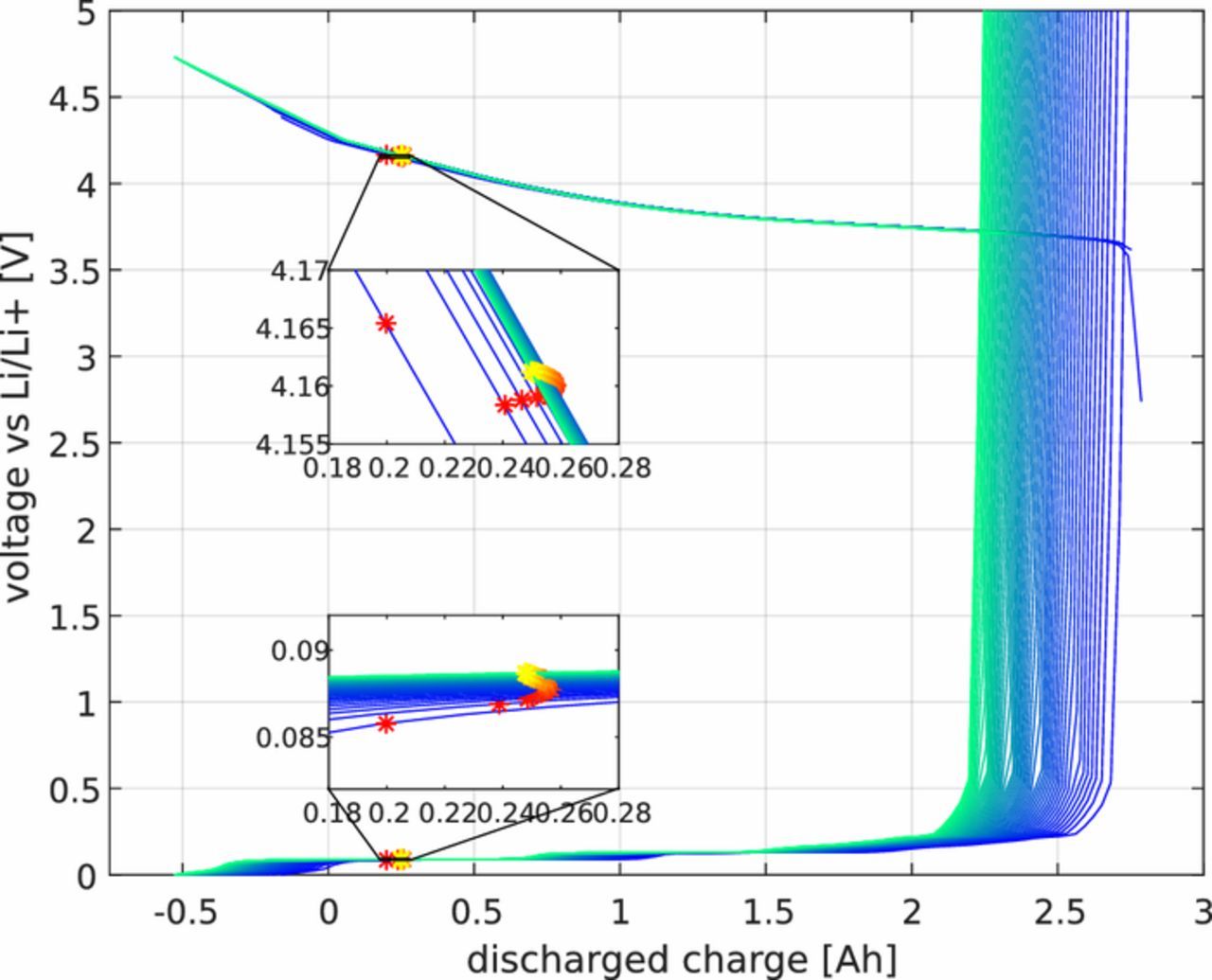
Figure 2. Half-cell OCV curves of a cell cycled at 1C and 25 degrees in an SoC window of 10% and 90%. The yellow-red stars shows the half-cell potential at the charged state (at 90% SoC). Blue and red show the OCV at the beginning of life, while yellow and green show the OCV at the end of life.
A challenge with implementing some of these degradation models is that they depend on cycle count rather than time. In degradation experiments with well defined cycles, this might be possible. But when real-life battery usage is predicted, it is very difficult to define what a single cycle means. Some researchers have used rainflow counting to solve this problem,1,83 but so far experimental proof that this is justified is lacking. For the purpose of this work, it was assumed that there is a linear relationship between the cycle count and calendar time in order to make the results more general without deviating too much from the original models.
Similarly, some other models had to be adapted to fit within the framework of this paper. The Li-fraction evolves monotonically during a half cycle, so Equation 18 can be approximated by using the difference in Li-fraction between the previous and present time steps, which will give the difference between minimum and maximum values over the entire cycle. A similar approach was followed for Equation 17, where it was additionally assumed that the effect was to increase the crack surface area  rather than directly decreasing the capacity. The full implementation of the code is available on GitHub.15
For the rest of this paper, capacity is defined as the charge accessible in a cell between the allowed voltage limits. In the experiments, it is measured by integrating the current whilst charging the cell from its lower voltage limit to the maximum voltage with a constant current constant voltage (CC-CV) profile. In the simulations, the same CC-CV charge between the same voltage limits is simulated and the simulated 'measured' capacity is then the integral of the current during this charge. Both in the experiments and simulations, such a capacity check is done after a predefined number of cycles.
Results and Discussion
Degradation data and parameter fitting
The simulations according to the various models are now compared with experimental data from two cells. A small number of degradation experiments had been conducted by various partners in the EU Everlasting project84 using a high-energy LG Chem NMC 18650 cell (INR18650 MJ185). This cell was cycled with a constant current, both on charge and on discharge, at 25°C. This was done between 10 and 90% state of charge (SoC). The data used in this paper is from a cell which was charged at 1C and discharged at 1.5C.
A larger degradation experiment had also been conducted by various partners in the EU Mat4Bat project86 using a high power Kokam NMC prismatic cell (SLPB78205130H87). These cells were cycled with a constant current and constant voltage charge, and a constant current discharge. This was at various temperatures, and between various SoC windows.3
The parameters of the SPM were fitted twice, once for each cell type. This was done manually by comparing the simulated and measured voltage during charging and discharging at various currents. The fitting parameters of the degradation models were set differently for every result shown below in order to match the simulations with the data. For example, when only SEI growth is considered, the values of the diffusion constant  and the exchange current density
  were set such that the predicted degradation matched the data. When later SEI growth was combined with other degradation mechanisms, such as surface cracking, the diffusion constant and exchange current density were changed such that the total predicted degradation fitted the data.
The parameters β and m (with various subscripts) have no direct physical interpretation and were therefore not constrained to any range. The parameters k and D (with various subscripts) are rate and diffusion constants which could be measured in theory, although this would be near impossible in practice.16,37,48 Therefore, most papers treat them as fitting parameters. The reported values in the literature have a huge range, e.g. for the rate constant of the SEI growth reaction,  , values between 10− 8 and 10− 16 have been reported.
Classification of degradation models
Three basic trends can be observed within existing lithium-ion battery degradation data sets. Some types of cells degrade faster at the start of life and their degradation rate decreases later in life.88,89 The degradation behavior of other cells is more linear with time, with rate of capacity decrease being approximately constant for a fixed usage pattern.90,91 Other cells show an accelerating degradation, especially toward the end of their lifetime when the capacity suddenly decreases very strongly.48,78,92 Sometimes, different operating conditions can lead to different degradation trends for the same cell type.
The degradation model equations previously introduced determine the trend of degradation over time and with usage. The kinetically limited SEI growth model (Equation 11) will produce a constant capacity fade for fixed usage because the magnitude of the side reaction current is broadly independent of the past degradation. On the other hand, the diffusion limited SEI growth model (Equation 13) will predict a decreasing rate of degradation for fixed usage because the magnitude of the side reaction current is inversely proportional to past degradation, represented by the thickness of the existing SEI layer δ, which will produce a square root of time dependency.
Laresgoiti's model for surface cracking (Equation 17) will give a constant degradation trend because the stress is not affected by previous crack growth. The same applies for Deshpande's model (Equation 18). Barai's crack growth model (Equation 19) will give a decreasing trend because the bigger the crack surface, the smaller the remaining possible active area for crack growth  . Ekstrom's model (Equation 21) will result in a constant degradation trend for the same reason as the kinetically limited SEI growth model.
There is more variability in the effects of the models for loss of active material. The physical stress model from Dai et al. coupled with a proportional degradation model from Laresgoiti et al. (Equations 22 to 25) will give a strongly accelerating degradation trend with time, because the more active material is lost, the higher the current density, the higher the Li-concentration gradients, the higher the stress, and the higher the decrease in porosity. For similar reasons, Delacourt's model (Equation 26) will also give an increasing trend but according to a square root. On the other hand, Narayanrao's loss of active material model (Equation 27) will give an exponentially decreasing trend because the smaller the effective surface a, the less it will decrease. Kindermann's model for electrode dissolution (Equation 28) will give a constant degradation rate, just like kinetically limited SEI growth. Finally, the Li-plating model (Equation 32) predicts a more or less constant degradation rate, because the rate of lithium plating does not depend on the previous amount of plated lithium.
As an example, Fig. 3 shows the different models classified by the trends they predict, along with a data set for each trend. None of the surface crack growth models are included because surface cracks don't decrease the capacity on their own. They only enlarge the surface area, and it is the SEI growth on this additional surface which will cause extra degradation. Therefore, crack growth models only cause extra degradation when they are combined with a model for SEI growth. It should be noted that the different trends can be difficult to see in the simulation results of Fig. 3 because in some cases the rate of change of the gradient is very gradual within the window shown. For instance, the capacity loss according to an exponential process is more or less linear at the start of the battery life (since y = e− t/τ ≈ 1 − t/τ for large τ and small t). Some exponential processes can decrease the capacity very suddenly, as is the case for Delacourt's LAM model. At the last successful capacity check in the simulation, the cell still had about 70% remaining capacity but then the cell degraded very quickly until it had no more remaining capacity. As was noted before, the equation for the electrolyte oxidation at the cathode is almost identical to Kindermann's model for LAM, explaining why their predictions are so similar.
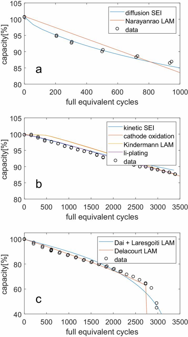
Figure 3. Basic degradation trends of the individual degradation models. The black markers are experimental results as described in the section about degradation data, while the lines are the simulations according to the various models. (a) Decreasing degradation rate for the LG Chem cell; (b) constant degradation rate for the Kokam cell cycled at 25°C at a 1C charge and 1C discharge between 10 and 90% SoC; (c) increasing degradation rate the Kokam cell cycled at 45°C at a 3C charge and 1C discharge between 0 and 100% SoC.
Combined models
Fig. 4 shows an example set of results when an SEI growth model is combined with one other degradation model. As explained in the section on degradation data and parameter fitting, the parameters for the degradation models were set differently for every combination of models in order to give a best fit against the available data. For reference, the solid lines show the degradation according to the SEI model alone; each different color represents a different value of the diffusion constant and/or exchange current density in the model. The dashed and dotted lines give combinations of SEI models with one other model, as indicated, such that the difference between the dashed/dotted and solid lines represents the additional degradation due to the second degradation model. The data and load cycles are the same as for Fig. 3.
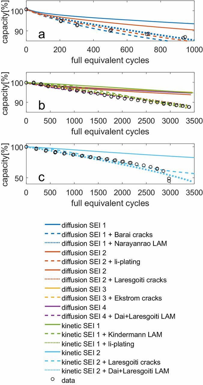
Figure 4. The dashed and dotted lines show the results of combining an SEI model with one other degradation model. For reference, the solid line of the same color indicates the degradation according to the SEI model only. The different colors represent SEI models with different diffusion constants and/or exchange current densities. The black data points are the same as in Fig. 3. (a) Decreasing degradation rate; (b) Constant degradation rate; (c) Increasing degradation rate.
The combination of a diffusion limited SEI growth model (which results in decelerating degradation over time) with another decelerating or linear degradation model produces a decreasing trend over time. Combining a diffusion limited SEI model with an accelerating degradation model produces a constant degradation rate if the rates of acceleration and deceleration are similar. The same effect also results from combining two models each having a constant degradation rate. Adding an accelerating degradation model to a kinetically limited SEI growth model produces an accelerating trend. The crack growth models are a slight exception: the SEI layer grows on the total electrode surface area, implying that the degradation rate is proportional to the integral of the crack growth rate. Therefore, a crack growth model with a constant crack growth rate will give an increasing degradation trend.
When implementing the combination of two models, it is important to include the feedback mechanisms between them. For instance, if the active material of the graphite electrode decreases due to a LAM degradation model, the current density for the same applied current will increase. This will lead to higher overpotentials, which will enhance the SEI growth if a kinetically limited SEI growth model is used. This effect is shown on Fig. 5, with Fig. 5a indicating the SEI layer thickness and Fig. 5b indicating the electrode surface area. The SEI thickness is determined by Equation 14, where the values of M and ρ have been taken from Pinson et al.37 The absolute thickness is not of importance in the model given that all the fitted transport parameters appear relative to the thickness in the equations, e.g.  . In other words, only the ratio of the fitted transport parameter to the thickness is of importance in determining the degradation behavior. The blue area shows the model results when only the SEI growth is modeled. As can be seen, the electrode surface area does not change in this scenario, and the layer thickness grows almost linearly with cycling, assuming it is only kinetically limited. The yellow area shows the increase in the SEI layer growth and surface area respectively when LAM is modeled alongside SEI growth. Although the LAM model alone produces a constant degradation rate, when combined with the SEI growth model it results in an accelerating growth rate. This is for the same reason as for crack growth described in the previous paragraph, namely the SEI growth rate is inversely proportional to the total active material, which is linearly decreasing, not to the rate at which this material is lost, which is constant. Note that this feedback mechanism does not exist when a purely diffusion limited SEI growth model is used because in that case, higher overpotentials do not lead to higher SEI growth rates. There are other similar cases, e.g. when the diffusion constant is reduced due to crack growth as given by Equation 20 and active material is lost due to a physical stress model which is given by Equations 22 to 25.
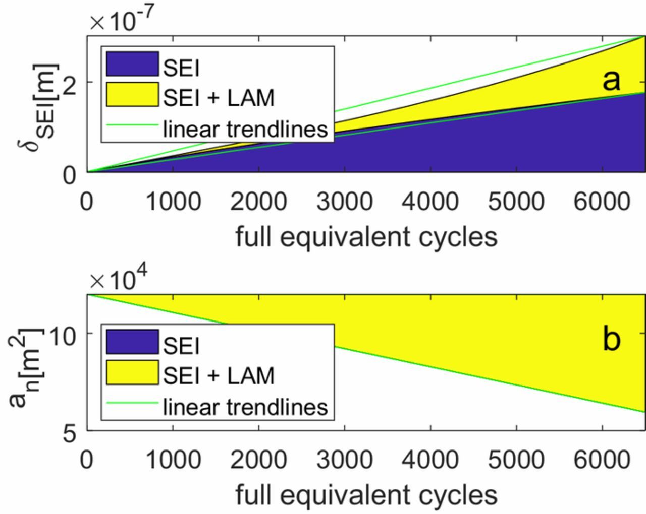
Figure 5. Feedback between kinetically limited SEI growth and LAM. The blue area is the effect when only SEI growth is considered, while the yellow area gives the additional effect when both SEI growth and LAM are considered. (a) Thickness of the SEI layer; (b) Effective surface area.
Negative feedback also exists, for example between kinetically limited SEI growth and Li-plating. Both models remove cyclable lithium, which increases the anode potential, while both are enhanced by lower voltages with respect to Li. This means that if there is more/less SEI growth, the anode potential is higher/lower and there will be less/more Li-plating.
Finally, either electrode can be limiting. For example, Kindermann's degradation model, given by Equation 28, acts on the cathode, while the SEI growth models decrease the anode capacity by removing Li-ions irreversibly. If the SEI model is dominant, the capacity is limited by the anode, and adding Kindermann's degradation model will have no effect on the overall capacity and vice versa.
Dependence of degradation on usage
It is well known that battery degradation is influenced by operational usage factors such as current, SoC and temperature.1,4 The different models of degradation respond very differently to varying operating conditions, as shown in Fig. 6.
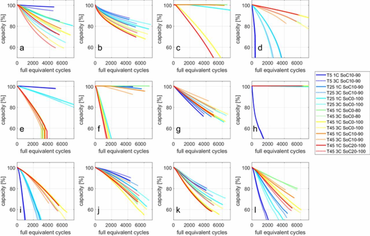
Figure 6. Dependencies of the various degradation models on usage. Each subplot gives the predictions according to one model, with the exception of the crack growth models which are combined with a diffusion limited SEI growth model. Discharge is at 1C, and charging is CC CV at various currents indicated by the legend. Ambient temperatures and SoC windows are indicated in the legend too. (a) Kinetically limited SEI growth, Equation 11; (b) Diffusion limited SEI growth, Equation 13; (c) Kinetically limited cathode solvent oxidation, Equation 29; (d) Dai + Laresgoiti LAM, Equations 22 to 25; (e) Delacourt LAM, Equation 26; (f) Kindermann LAM, Equation 28; (g) Narayanrao LAM, Equation 27; (h) Li-plating, Equation 32; (i) Diffusion limited SEI growth + Deshpande crack growth, 18; (j) Diffusion limited SEI growth + Laresgoiti crack growth, Equation 17; (k) Diffusion limited SEI growth + Barai crack growth, 19; (l) Diffusion limited SEI growth + Ekstrom crack growth, Equation 21.
The kinetically limited SEI growth model predicts increased degradation at high current, high SoC and high temperature, especially if the temperature dependency of the rate constant is explicitly considered, similar to Equation 9. The diffusion limited SEI growth model is however independent of current and SoC and will only give higher degradation at higher temperature, again on the condition that the temperature dependency of the diffusion constant is considered, similar to Equation 8. Therefore, in the case of diffusion limited SEI growth, the degradation of all cycles with the same temperatures maps onto a single line if plotted against time on the x-axis. However, the x-axis of Fig. 6 is 'full equivalent cycles' (FEC), which is the total charge throughput divided by twice the nominal cell capacity. Because the different cycles take different amounts of time, the prediction does not map to a single line per temperature. This shows how changing the independent variable can reveal different trends in degradation data, which might be useful to identify which degradation models fit the data best.
The model for electrolyte oxidation behaves as a mix of the kinetically limited SEI growth model, Equation 11, and Kindermann's cathode dissolution model, Equation 28. The SoC is by far the most important factor, with more degradation at high SoC.
There is a large difference between the results of the various models for crack growth as well as between the various models for LAM. The most important difference is how much the stress is affected by the change of the diffusion constant due to changing temperatures. Lower temperatures and corresponding lower diffusion constants will always lead to larger spatial concentration gradients inside the active material, as well as to faster concentration swings on the surface of the electrode. Desphande's crack growth model and Dai's LAM model, respectively Equations 18 and 22 to 25, are more sensitive to this than Laresgoiti's crack growth model (Equation 17). Other models are independent of any operating condition, such as Narayanrao's LAM model (Equation 27). Such models will predict identical degradation for all cycles of the same temperature, but because the independent variable is FEC instead of time, the degradation for each cycle looks different. The more empirical models such as Equations 19 and 26 typically only depend on the current and temperature, and given that the independent variable is proportional to the charge throughput, this means all predictions for the same temperature map almost to a single line. The models using Tafel equations (Equations 21, 28 and 32) have the same dependencies as the kinetically limited SEI growth model although the temperature dependency of Equations 21 and 32 is negative instead of positive.
Fig. 7 demonstrates how a combination of various models can generalize to match most of the trends observable in the large data set recorded for the Kokam cell. The generalized model illustrated here is a combination of diffusion limited SEI (Equation 13), Delacourt's LAM model (Equation 26), Kindermann's model for cathode dissolution (Equation 28) and Yang's model for Li-plating (Equation 32). All the models interact with each other as explained previously. The values of the fitting parameters of the models used here are given in table II. A best fit of this generalized model is shown across the entire experimental data set. The Li-plating model ensures the rapid degradation at low temperature is captured, but fails to capture the later decreasing degradation trend fast enough. It is unclear why this happens, but probably some negative feedback mechanism prevents further plating in the real cell, which is not included in the model. The cathode dissolution model explains the degradation for cycles at high SoC windows, and the combination of the SEI layer growth model and loss of active material model explains the remaining degradation trends.
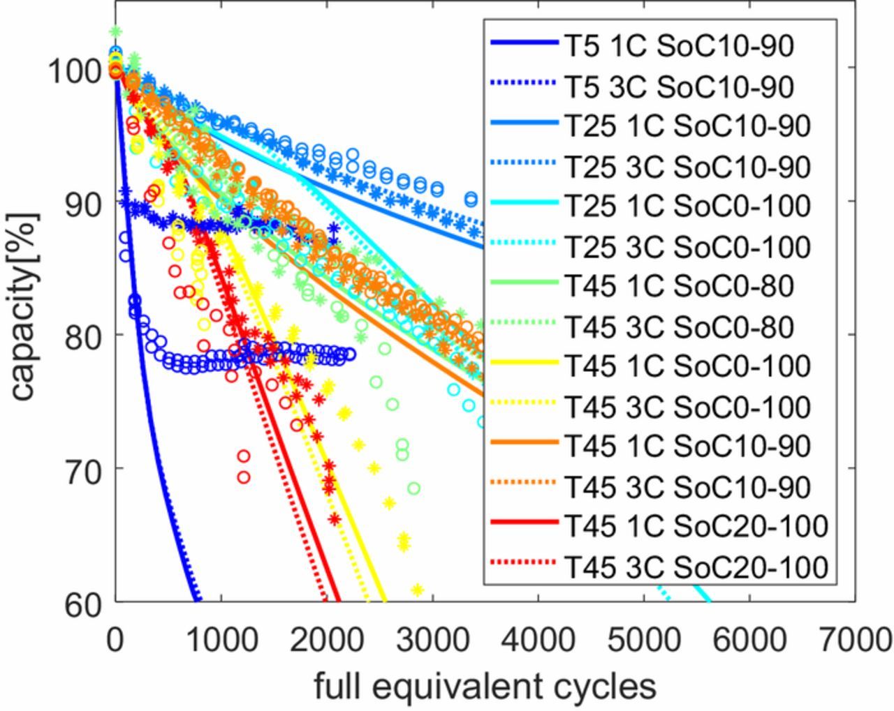
Figure 7. Degradation predictions for various cycling regimes, comparing a generalized model (lines) vs. measured degradation data from Kokam cells with the same cycling regimes as in Fig. 6 (circles for 3C data, asterisks for 1C data). The generalized model combines a diffusion limited SEI model, Delacourt's LAM model, Kindermann's model for cathode dissolution and Yang's model of Li-plating.
Table II. Fitted parameters of the generalized degradation model.
| Parameter | Symbol | Value | unit |
|---|---|---|---|
| Rate constant of the SEI reaction |  |
2.75e-13 | m s− 1 |
Arrhenius constant of  |
 |
130,000 | J mol− 1 |
| Diffusion constant of the SEI reaction |  |
1.125e-14 | m2 s− 1 |
Arrhenius constant of  |
 |
20,000 | J mol− 1 |
| Fitting constant in Delacourt's LAM model | β7 | −1.675e-5 | m2 C− 1 |
| Arrhenius constant of β7 |  |
54,611 | J mol− 1 1 |
| Fitting constant in Delacourt's LAM model | β8 | 0 | m C− 0.5 s− 0.5 |
| Relative exchange current density of Kindermann's LAM model |  |
1.25e-05 | A mol− 1 |
Arrhenius constant of  |
 |
27,305 | J mol− 1 |
| Rate constant of the plating reaction |  |
2.25e-10 | A m− 2 |
Arrhenius constant of  |
 |
−201,400 | J mol− 1 |
Conclusions
In this work, many different physical degradation models from literature were implemented within a single particle model framework. When looking at the partial differential equations of the models, it is straightforward to identify the basic degradation trend that each will predict: a decreasing, constant, or increasing degradation rate.
Combining two degradation models might result in a different degradation trend. For instance the combination of one model with decreasing and one with increasing degradation trends can result in a constant degradation rate. However, feedback mechanisms between the models might alter the trends that would normally be expected. For instance, the positive feedback between a kinetically limited SEI growth model and a LAM model, both of which have a constant degradation trends, results in an increasing trend. Also negative feedback mechanisms exist, for instance between lithium plating and kinetically limited SEI growth.
When considering a small degradation data set, it might seem as if all the models behave similarly and all can predict the observed degradation. But when variable cycling conditions are simulated, the differences between the models become apparent. Fitting a large data set requires multiple degradation models to capture the different degradation trends observed for different operating conditions. Therefore, when deciding which degradation model to choose to explain a given data set, or to determine how accurate a model might be, the largest data set possible should be used, and extremes of behavior should be captured in addition to normal behavior. It is insufficient to compare the simulations with data for only a few cycling regimes.
Acknowledgments
This work was supported by VITO and EnergyVille, Belgium. The research leading to these results was performed within the MAT4BAT project (http://mat4bat.eu/) and received funding from the European Union Seventh Framework Programme (FP7/2007–2013) under grant agreement no. 608931 and under the SolSThore project which receives the support of the European Union, the European Regional Development Fund ERDF, Flanders Innovation & Entrepreneurship and the Province of Limburg. Financial support was also received from EVERLASTING project in the Horizon 2020 program of the European Union under the grant 'Electric Vehicle Enhanced Range, Lifetime And Safety Through INGenious battery management' (EVERLASTING-713771).
ORCID
Jorn M. Reniers 0000-0002-4186-8696
David A. Howey 0000-0002-0620-3955