Abstract
Polymer-electrolyte fuel cells are a promising energy-conversion technology. Over the last several decades significant progress has been made in increasing their performance and durability, of which continuum-level modeling of the transport processes has played an integral part. In this review, we examine the state-of-the-art modeling approaches, with a goal of elucidating the knowledge gaps and needs going forward in the field. In particular, the focus is on multiphase flow, especially in terms of understanding interactions at interfaces, and catalyst layers with a focus on the impacts of ionomer thin-films and multiscale phenomena. Overall, we highlight where there is consensus in terms of modeling approaches as well as opportunities for further improvement and clarification, including identification of several critical areas for future research.
Export citation and abstract BibTeX RIS

This is an open access article distributed under the terms of the Creative Commons Attribution 4.0 License (CC BY, http://creativecommons.org/licenses/by/4.0/), which permits unrestricted reuse of the work in any medium, provided the original work is properly cited.
Fuel cells may become the energy-delivery devices of the 21st century. Although there are many types of fuel cells, polymer-electrolyte fuel cells (PEFCs) are receiving the most attention for automotive and small stationary applications. In a PEFC, fuel and oxygen are combined electrochemically. If hydrogen is used as the fuel, it oxidizes at the anode releasing proton and electrons according to
![Equation ([1])](https://content.cld.iop.org/journals/1945-7111/161/12/F1254/revision1/jes_161_12_F1254eqn1.jpg)
The generated protons are transported across the membrane and the electrons across the external circuit. At the cathode catalyst layer, protons and electrons recombine with oxygen to generate water
![Equation ([2])](https://content.cld.iop.org/journals/1945-7111/161/12/F1254/revision1/jes_161_12_F1254eqn2.jpg)
Although the above electrode reactions are written in single step, multiple elementary reaction pathways are possible at each electrode. During the operation of a PEFC, many interrelated and complex phenomena occur. These processes include mass and heat transfer, electrochemical reactions, and ionic and electronic transport.
Over the last several decades significant progress has been made in increasing PEFC performance and durability. Such progress has been enabled by experiments and computation at multiple scales, with the bulk of the focus being on optimizing and discovering new materials for the membrane-electrode-assembly (MEA), composed of the proton-exchange membrane (PEM), catalyst layers, and diffusion-media (DM) backing layers. In particular, continuum modeling has been invaluable in providing understanding and insight into processes and phenomena that cannot be resolved or uncoupled through experiments. While modeling of the transport and related phenomena has progressed greatly, there are still some critical areas that need attention. These areas include modeling the catalyst layer and multiphase phenomena in the PEFC porous media.
While there have been various reviews over the years of PEFC modeling1–7 and issues,8–14 as well as numerous books and book chapters, there is a need to examine critically the field in terms of what has been done and what needs to be done. This review serves that purpose with a focus on transport modeling of PEFCs. This is not meant to be an exhaustive review of the very substantial literature on this topic, but to serve more as an examination and discussion of the state of the art and the needs going forward. In this fashion, the review focuses a bit more on the recent modeling issues and advances and not as much on the various approaches that are historical or outside the scope of current issues.
This review is organized as follows. First, some background introduction into PEFC transport modeling is accomplished including the general governing equations, modeling dimensionality, and a discussion on empirical modeling and the dominant mechanisms, with a focus on the generalized governing equations for the different mechanisms and phenomena. Next, we critically examine multiphase-flow and catalyst-layer modeling. For the former, we will introduce several treatments and then focus on current issues including effective properties, some microscale modeling, phase-change behavior, and the impact and existence of interfaces. For catalyst-layer modeling, we discuss incorporating structural details into the modeling framework, and focus on consideration of ionomer thin-films, as well as transport in ionomer-free zones, and finally touch on the intersection between transport modeling and durability. The next section focuses on future perspectives including interactions between modeling and experiments, modeling variability, open-source modeling, and an overall summary of the article.
Background
In this section, some background information is provided in order to orient the reader for the more detailed discussions below concerning multiphase-flow and catalyst-layer modeling and phenomena. As noted, the physics of most models is similar with the differences being in the scale of the model and phenomena investigated, treatment of the various transport properties, and boundary conditions. In this section, first a discussion of model dimensionality is made, followed by a general description and review of macroscale, empirical modeling. Finally, the general governing equations are presented. As noted above, within this section the focus is on the state-of-the-art equations for the different mechanisms, layers, and phenomena, and not on the specific models that have been used and which models have used which equations. Thus, the equations presented are generalized and classified and represent the key foundational precepts that are required for a more in-depth investigation into the critical phenomena in the following sections.
Although this is a review focused on transport modeling, one needs to be aware of the thermodynamics of the cell. From this perspective, a PEFC converts the intrinsic chemical energy of a fuel into electrical and heat energies. The associated Gibbs free energy can be converted to a potential by
![Equation ([3])](https://content.cld.iop.org/journals/1945-7111/161/12/F1254/revision1/jes_161_12_F1254eqn3.jpg)
where nh is the number of electrons transferred in reaction h and F is Faraday's constant. Similarly, one can define the enthalpy potential as
![Equation ([4])](https://content.cld.iop.org/journals/1945-7111/161/12/F1254/revision1/jes_161_12_F1254eqn4.jpg)
and thus the total heat released by the PEFC can be given by
![Equation ([5])](https://content.cld.iop.org/journals/1945-7111/161/12/F1254/revision1/jes_161_12_F1254eqn5.jpg)
where V is the cell potential. Thus, if the cell potential equals the enthalpy potential, there is no net heat loss/gain. As reference, for hydrogen and oxygen going to liquid water at standard conditions, the reversible and enthalpy potentials are 1.229 and 1.48 V, respectively. To change to different conditions for this reaction, one can use thermodynamic expressions for temperature as well as a Nernst equation for composition,
![Equation ([6])](https://content.cld.iop.org/journals/1945-7111/161/12/F1254/revision1/jes_161_12_F1254eqn6.jpg)
where ai is the activity of species i, and R is the ideal-gas constant. From thermodynamics, the equilibrium and enthalpy potentials depend on the phase of water produced (i.e., liquid or vapor), and in this review it is assumed that water is produced in the condensed (liquid) phase next to the membrane (i.e.,  in equation 6). Since the associated liquid and vapor cell potentials are related by the vapor pressure of water, there is no issue in assuming a vapor product as long as the heat of vaporization/condensation is accounted for in the energy balance.
Model Dimensionality
Just as with scale, there is an issue of model dimensionality in that higher dimensional models better represent reality but at a greater computational expense. A lower-dimensionality model sacrifices some spatial fidelity but often allows for more complex physics to be incorporated. Due to increases in computational power, more multi-dimensional models are being employed, with perhaps the ideal tradeoff being the 1+2-D model framework. Figure 2 displays the various model dimensionalities and major cell components.
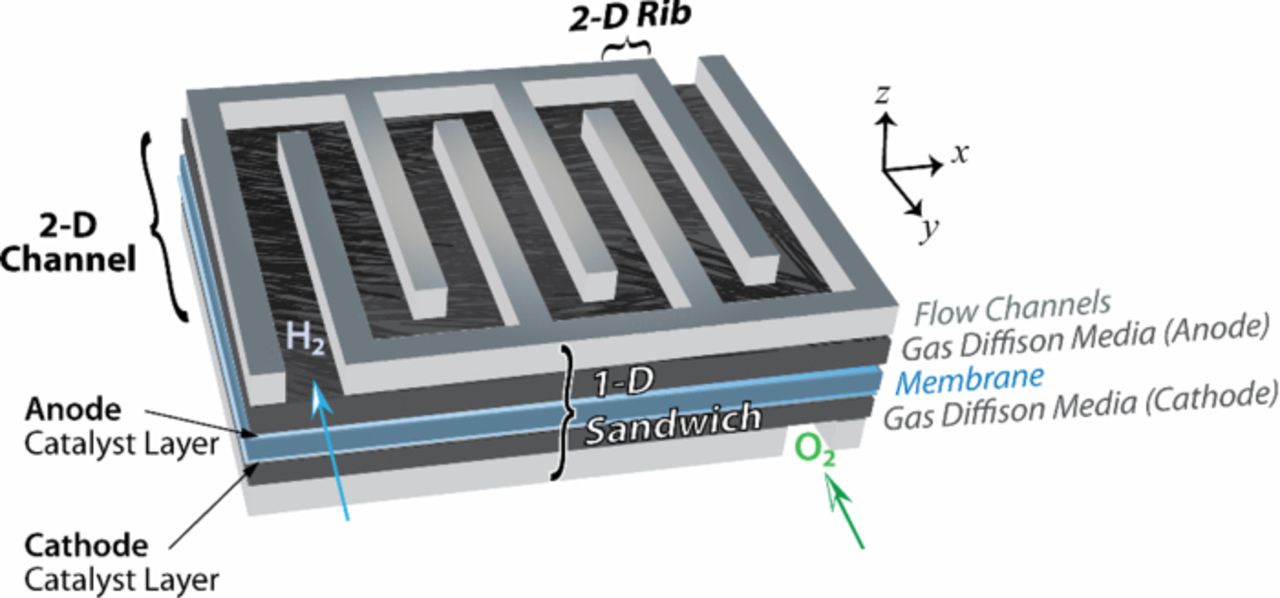
Figure 2. Schematic of spatial domains and associated modeling including the PEFC sandwich.
Zero-dimensional (0-D) models relate system variables such as cell voltage, current, temperature, pressure, gas flow rate or any other property using simple empirical correlations without any consideration of the spatial domain. 0-D models are used to determine kinetic and net ohmic resistance parameters from a polarization performance curve.15–22 A typical 0-D model equation for a polarization curve is
![Equation ([7])](https://content.cld.iop.org/journals/1945-7111/161/12/F1254/revision1/jes_161_12_F1254eqn7.jpg)
and accounts for the major losses as shown in Figure 1. The first term on the right corresponds to the thermodynamic cell potential. The second and third terms represent the loss in cell potential to kinetic resistance where b is the effective Tafel slope. The fourth term accounts for the loss to ohmic resistance, R', and the last represents the limiting current caused by concentration overpotential. As 0-D models do not provide fundamental understanding of PEFC operation, they have limited suitability for predicting performance for different operating conditions or optimizing the design. Empirically-based models are often 0-D models and can allow for some prediction of behavior of a specific material set under certain operating windows as discussed below.
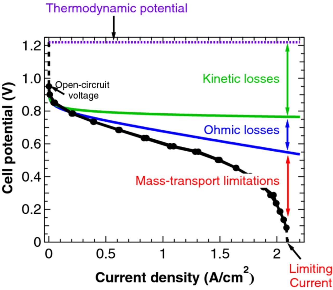
Figure 1. Sample polarization curve showing dominant losses.
One dimensional (1-D) models describe the physical phenomena occurring in one spatial dimension typically across the membrane-electrode assembly.23–25 Comprehensive 1-D models incorporate electrochemical reaction at the porous electrodes, transport of gas and liquid species through porous gas-diffusion media (DM) or porous-transport layers (PTLs), and transport of charged species like electrons and protons. Proper interfacial internal boundary conditions are used to couple the different processes across layer boundaries. Along-the-channel 1-D models focus on the transport and depletion of fuel and oxygen along the channel and its effects on current density.
Two-dimensional models use the 1-D model direction and another direction (across-the-channel or along-the-channel).1 Across-the-channel models focus on a cross section of the flow channel including the rib and channel. This approach addresses the effects of the solid rib and channel on the distribution of species such as electrons and water. As the rib is essentially a current and heat collector, its contact with the gas-diffusion layer (GDL) blocks that portion of it to the gas channel. This reduces the mass transport to and from the electrode region directly underneath the rib. Along-the-channel 2-D models incorporate the effect of fuel and oxygen depletion and water accumulation on the current distribution along the channel and across the cell sandwich. Distribution of water, temperature, and reacting species within the PEFC can be predicted by the model. This also helps in understanding the different types of channel configuration and flow direction which cannot be addressed with 1-D modeling. Most of the 2-D models assume that the flow channel can be approximated as a straight channel. Such an assumption may ignore the transport through the porous media under the ribs (e.g., for serpentine channels), but simplifies the model greatly. One can also use arguments of spatial separation to assume that the conditions in the cell sandwich only propagate and interact along the channel and not by internal gradients. This finding led to a group of models referred to as pseudo-2-D or 1+1-D models. Instead of solving the coupled conservation equations in a 2-D domain, the 1-D model is solved at each node along the channel. This reduces the computational requirement without the complexity of solving the equations in a 2-D domain.
The significant decrease in computing costs has promoted complex and computationally intensive numerical modeling including full 3-D models. In addition to understanding distribution of species and current, these models show the distribution of temperature and fluid in the 3-D spatial domain, especially the effect of cooling channels, channel cross section, and channel turn effects. Similar to pseudo 2-D models, there is also a class of models termed pseudo 3-D or 1+2-D. In this formulation, the along-the-channel direction is only interacting at the boundaries between cell components, but instead of 1-D sandwich models, 2-D across-the-channel models are used. Such a structure is probably the best tradeoff between computational cost and model fidelity.
While the above classification is geared more toward macroscale modeling, similar delineations can be made on the microscale, where continuum equations are still used and remain valid. Typically, these models have much smaller domains and are often of higher dimensionality since they are focused on specific phenomena. For example, modeling transport at the local scale of ions through a catalyst layer often requires 2-D and 3-D models to account for the correct geometry and geometry-dependent physics. Finally, one can also examine multiscale models as being multi-dimensional. For example, as mentioned, there are 3-D models at the microscale that can determine properties which are subsequently used in a macroscale model that maybe is a 1-D model. Also, within the porous catalyst layer (see section below), typically one uses an expression or submodel for reaction into the reactive particle as well as across the domain, which, when taken together, can be considered as two separate dimensions.
Empirical-Based Modeling
As discussed above, there is extensive literature on modeling of transport processes in PEFCs and at various dimensions and physics. The approach currently taken by many fuel-cell developers is to first develop a comprehensive database from experiments conducted on a well-defined, representative material system. These experiments focus on in-situ and ex-situ measurement methods with resolution normal to the membrane to quantify transport processes at critical material interfaces, in addition to bulk-phase transport. Based on these component-level studies, models are developed in a simplified computational package that can be effectively used as an engineering tool, for assessment of the effects of material properties, design features, and operating conditions on PEFC performance.26 Such models are often classified as 0-D, although they can contain more detailed descriptions of the physics from the experiments. Thus, the model is of the form
![Equation ([8])](https://content.cld.iop.org/journals/1945-7111/161/12/F1254/revision1/jes_161_12_F1254eqn8.jpg)
where ηHOR is the kinetic loss from the HOR, ηORR is the kinetic loss from the ORR,  is the ohmic loss from electron transport,
  is the ohmic loss from proton transport, and ηtx is the mass-transport loss. The reversible potential is often determined empirically from the open-circuit voltage or by a thermodynamic expression. The kinetic overpotentials can be determined based on experimental measurements of Tafel slopes (see equation 7). With regard to transport, researchers are focused on quantifying and modeling the last three transport terms in equation 8, which can be compared to the associated expressions given by equation 7. Electron, ion (proton), and mass transport are all strongly influenced by water transport and early work in collecting these losses for a comprehensive model was limited to operating conditions where the relative humidity (RH) was less than 100% or the impact of liquid-water accumulation was not accounted for explicitly.27 However, because of the effect of even small temperature gradients on water transport and phase change, the thermal transport resistance and the resulting saturation gradients are now being considered in parametric fuel-cell models.28,29 Below, we detail the various expressions and touch on empirical methods to obtain them.
Electronic resistance
The ohmic loss associated with the mobility of electrons is most strongly influenced by the contact resistances between the various diffusion layers with only a small contribution from the through-plane bulk electrical resistance. This resistance can be measured using the as-made GDM, typically consisting of both the GDL and microporous layer (MPL). To measure the resistance, two sheets of GDL with the MPLs facing each other are placed in a fixture with compression plates made of the flow field (current collector) material and geometry.30 For a given stress, this experiment results in a lumped electrical resistance that consists of all contact resistances along with the weighted average of the through-plane and in-plane bulk resistances as they apply to the flowfield geometry. For a more detailed model or multi-dimensional approaches, the in-plane and contact resistances are measured independently.31 The bulk electrical resistance in the relatively thin electrode is negligible.
Protonic resistance
In addition to the electronic resistance through the solid phase, the protonic resistance through the PEM is part of the total ohmic resistance. The protonic resistance has a strong dependence on the RH in the adjacent electrodes and is only a weak function of temperature.32 The membrane conductance as it varies with RH can be characterized by in-situ33 or ex-situ34 methods. Furthermore, the sum of the electronic and protonic resistances is normally validated with AC impedance at high frequency during PEFC experiments at various operating conditions.
Resistance to proton transport also occurs in the dispersed electrodes where a thin film of electrolyte is responsible for a lateral transport relative to the membrane plane. In addition to being a function of RH (as with the membrane), this resistance is also dependent on current density due to the variation in electrode utilization depth as current draw increases.35 The electrode effectiveness can be modeled theoretically with Tafel kinetics, and this is used to correct an area-based proton resistance in the anode and cathode electrodes which is commonly measured with H2/N2 AC impedance32 and an associated transmission-line model.36 This method of characterizing the proton resistance in the electrode requires an assumption of uniform ionomer film thickness and connectivity. The ionomer film is difficult to characterize, and if this film was discontinuous with significant variations in thickness, the idealized proton resistance would under-predict the loss associated with proton mobility in the electrode. The ionomer film and its associated effects are discussed in more detail in a later section.
Thermal resistance
All of the voltage loss terms in equation 8 have some functionality with temperature. To predict accurately the reaction kinetics and the gas composition at the catalyst surface, the temperature profile through the PEFC sandwich must be established. There are several methods for characterizing the bulk and contact resistances of PEFC components as reviewed by Zamel and Li37 and Wang et al.6 The total thermal resistance is used to solve the heat equation in one of two dimensions based on the heat flux from the cathode catalyst layer. At high RH conditions, where proton resistance is minimized along with the product water flux from the cathode catalyst layer, such an analysis elucidates regions of phase change within the open volume of the diffusion layers and gas-delivery channels.
Diffusion resistance
There are several length scales for which diffusion resistance must be characterized. For a given total pressure in the flow channel, the first resistance to mass transport is encountered at the GDL interface. The convective mass-transfer coefficient, computed from the Sherwood number for a given flow rate and channel geometry is used for single-phase conditions in the channel.38 The impact of liquid water in the gas channel is accomplish with a modified Sherwood number39 and by reducing the gas contact area using a surface-coverage ratio.40 In the GDM, the characterization of diffusion and governing parameters has been accomplished using various experiments combined with simple limiting-current or Fickian-type diffusion equations to get the values for use in equation 7 or 8.41–44 A more direct in-situ measurement of oxygen diffusion resistance has been presented in previous work by Baker et al.38 and Caulk et al.45 that established a method and analysis using limiting-current measurements under dry and oversaturated conditions for use in equation 7 or 8. Although these measurements result in a diffusion resistance while a two-phase condition exists in the PEFC assembly, the degree of saturation and its distribution is unknown; as a result, a direct correlation between saturation and the resulting change in the diffusion resistance is required to validate a simplified saturation model. The limiting-current analysis developed by Baker et al. can also be used to isolate the pressure-independent component of diffusion resistance (i.e., Knudsen diffusion and interfacial resistance through water/ionomer (combined with Henry's law)).38 Studies have shown that this interfacial resistance is a significant component of voltage loss as it scales with reduced platinum loading and that it is much higher than expected based on oxygen permeability through bulk ionomer as discussed in more detail in another section below.46–49 Currently in a parametric model, this resistance is accounted for by using an unrealistically thick ionomer or electrolyte layer with bulk ionomer (membrane) transport properties.
Membrane transport
Accurate prediction of the reactant partial pressure at the catalyst surface requires the solution of species throughout the PEFC assembly which is beyond the scope of empirical models. Although the thermal, electronic, protonic, and gas-phase transport resistances can be characterized, the water balance between the anode and cathode due to water permeation through the electrolyte must be accounted for. This water balance also complicates the prediction of phase change and most of the components of transport resistance are a function of the local liquid-water content. The key is to determine the net flux of water through the ionomer, which is a function of different driving forces including chemical potential and electro-osmosis driven by proton movement.50 For chemical-potential driven flow, there is still debate over the values of the transport coefficients and the possible existence of a humidity-dependent interfacial resistance in the membrane, where there is experimental support on both sides of the issue.51–68 The value of the electro-osmotic coefficient also varies significantly in literature,69–71 and since it scales with current density it plays a critical role in predicting the water balance. Given the above difficulties, many parametric models use an empirical effective electro-osmotic coefficient.
Along-the-channel solution
The various resistances described above are assembled in a through-plane model with boundary conditions at the flow distributors that include total pressure, species concentration, temperature, and a reference potential of 0 V at the anode current collector. The cathode current collector potential is calculated based on equation 8, where electronic and protonic resistances are used to predict the ohmic losses and the diffusion and thermal resistances are used to predict the species partial pressures and temperature in the catalyst layers for calculation of the half-cell potentials, reaction kinetics, and membrane transport. This is typically solved in 1-D with average values over the geometric features.
Practical PEFC stacks have significant variation in the channel boundary conditions from the inlet to the outlet. To account for this, the parametric model is applied along-the-channel, assuming equipotential current collectors or by using a correlation for lateral potential difference through the current collector. This solution requires an accurate prediction of flow resistance in the channel. Although straight-forward for single-phase conditions, a two-phase pressure differential correlation is required once the flow distributor condition exceeds 100% RH.72–75 Additionally, PEFC systems typically operate with hydrogen stoichiometric ratios greater than 1.0, thereby requiring a methodology for recirculating exhaust anode flow. In this case the nitrogen and water content in the anode flow distributor due to crossover through the membrane must be accounted for as the diluted hydrogen feed stream will impact performance.
Basic Governing Equations
The above sections describe the methodologies and dimensionalities for modeling PEFCs based on a good amount of empiricism. To model PEFC behavior with more detailed physics at the continuum scale requires the use of overall conservation equations for mass, momentum, energy, and charge transport within the various subdomains or components. In addition, there is a need for expressions for overall kinetics and thermodynamics. The general physics equations are more or less known and used in their general forms, with the complications arising from the need to determine the correct boundary conditions, effective properties, and related transfer expressions. In this section, the general governing equations are presented including the conservation laws along with the general, well-known transport equations. As mentioned, the equations presented below have not necessarily been used as is since they represent generalized forms of specific modeling approaches in order to be concise and show the generality of the phenomena being modeled. Also, no model has really used all of the governing equations below as most focus on certain aspects; however, we believe that these equations should be used and are the foundation for the more detailed discussions in subsequent sections.
For a control segment, the general conservation equation for property ψ, representing any of the aforementioned transport processes, can be written as
![Equation ([9])](https://content.cld.iop.org/journals/1945-7111/161/12/F1254/revision1/jes_161_12_F1254eqn9.jpg)
The first term represents the time-dependent property and is neglected for description of steady-state operation, which is the favored approach to understand the mechanisms involved. However when it comes to application-specific models – such as automobile applications involving start-stop cycles – dynamic models are better suited. While a vast majority of PEFC models are steady-state models, there are transient models that address specific transient phenomena such as degradation mechanism,76,77 contamination effects,78 dynamic load-change effects,79,80 operational anomalies, and start-stop cycles and freeze start,5,81,82 and describe the transition of properties or system variables affecting PEFC operation.
The second term in equation 9 represents the change in the property ψ due to flux (N) of ψ into or out of the control segment under study. The flux denotes the transfer of property driven by imbalances within the system and is the result of system adjusting itself to bring certain equilibrium.
The third term (S) called the source term represents all of the processes that cause generation or decay of the property within the control segment. For example, a supersaturated vapor phase may condense within the control segment and leads to a decrease in vapor-phase concentration and an increase in liquid-phase concentration. This term incorporates all other terms such as reaction terms and phase-change terms that are not captured by the flux. The term couples different conservation laws within the segment.
Material transport
The conservation of material can be written as in equation 9 except that the physical quantity ψ could be p – partial pressure of a gas, c – concentration in solution, x – mole fraction of a particular species, w – mass fraction of a particular species, or ρ – density of a fluid. However, for the case of a mixture in a multiphase system, it is necessary to write material balances for each component in each phase k, which in summation governs the overall conservation of material,
![Equation ([10])](https://content.cld.iop.org/journals/1945-7111/161/12/F1254/revision1/jes_161_12_F1254eqn10.jpg)
In the above expression, ɛk is the volume fraction of phase k, ci,k is the concentration of species i in phase k, and si,k,l is the stoichiometric coefficient of species i in phase k participating in heterogeneous reaction l, ak,p is the specific surface area (surface area per unit total volume) of the interface between phases k and p, and ih,l-k is the normal interfacial current transferred per unit interfacial area across the interface between the electronically conducting phase and phase k due to electron-transfer reaction h and is positive in the anodic direction. It should be noted that the above equation is a generalized form that covers what almost all models use for the material balance, albeit with specific terms substituted for the general ones as discussed in the next sections.
The term on the left side of the equation is the accumulation term, which accounts for the change in the total amount of species i held in phase k within a differential control volume over time. The first term on the right side of the equation keeps track of the material that enters or leaves the control volume by mass transport as discussed in later sections. The remaining three terms account for material that is gained or lost (i.e., source terms, Sψ, in equation 9). The first summation includes all electron-transfer reactions that occur at the interface between phase k and the electronically conducting phase 1; the second summation accounts for all other interfacial processes that do not include electron transfer like evaporation or condensation; and the final term accounts for homogeneous chemical reactions in phase k. It should be noted that in terms of an equation count, for n species there are only n−1 conservation equations (where n is the number of components) needed since one can be replaced by the sum of the other ones, or, similarly, by the fact that the sum of the concentrations equals the total concentration (i.e., sum of mole fractions equals 1),
![Equation ([11])](https://content.cld.iop.org/journals/1945-7111/161/12/F1254/revision1/jes_161_12_F1254eqn11.jpg)
where cT, k is the total concentration of species in phase k.
In the above material balance (equation 10), one needs an expression for the flux or transport of material. Often, this expression stems from considering only the interactions of the various species with the solvent
![Equation ([12])](https://content.cld.iop.org/journals/1945-7111/161/12/F1254/revision1/jes_161_12_F1254eqn12.jpg)
where Deffi is the effective diffusion coefficient of species i in the gas mixture and v*k is the molar-averaged velocity of phase k
![Equation ([13])](https://content.cld.iop.org/journals/1945-7111/161/12/F1254/revision1/jes_161_12_F1254eqn13.jpg)
Substitution of equation 12 into equation 10 results in the equation for convective diffusion,
![Equation ([14])](https://content.cld.iop.org/journals/1945-7111/161/12/F1254/revision1/jes_161_12_F1254eqn14.jpg)
which is often used (or its analogous mass-based form) in simulations. In the above expressions, the reaction source terms are not shown explicitly, and the superscript 'eff' is used to denote an effective diffusion coefficient due to different phenomena or phases as discussed later in this review. For example, to account for Knudsen diffusion primarily in the MPLs and catalyst layers, one can use a diffusion coefficient that is a parallel resistance83
![Equation ([15])](https://content.cld.iop.org/journals/1945-7111/161/12/F1254/revision1/jes_161_12_F1254eqn15.jpg)
where the Knudsen diffusivity is given by
![Equation ([16])](https://content.cld.iop.org/journals/1945-7111/161/12/F1254/revision1/jes_161_12_F1254eqn16.jpg)
where d is the pore diameter and Mi is the molar mass of species i. This diffusion coefficient is independent of pressure whereas ordinary diffusion coefficients have an inverse dependence on pressure. Additionally, the diffusion coefficient is often modified for the tortuosity or path length required for the diffusion to occur in a multiphase system,
![Equation ([17])](https://content.cld.iop.org/journals/1945-7111/161/12/F1254/revision1/jes_161_12_F1254eqn17.jpg)
where τk is the tortuosity of phase k and is greater than 1.
If the interactions among the various species are important, then equation 12 needs to be replaced with the multicomponent Stefan-Maxwell equations that account for binary interactions among the various species
![Equation ([18])](https://content.cld.iop.org/journals/1945-7111/161/12/F1254/revision1/jes_161_12_F1254eqn18.jpg)
where xi is the mole fraction of species i and Deffi, j is the effective binary diffusion coefficient between species i and j. The first term on the right side accounts for pressure diffusion (e.g., in centrifugation) which often can be ignored, but, on the anode side, the differences between the molar masses of hydrogen and water vapor means that it can become important in certain circumstances.84 The second term on the right side stems from the binary collisions between various components. For a multicomponent system, equation 18 results in the correct number of transport properties that must be specified to characterize the system, ½n(n−1), where the ½ is because Deffi, j = Dj, ieff by the Onsager reciprocal relations. Finally, the third term on the right side represents Knudsen diffusion effects when incorporated rigorously and using the solid phase as the reference velocity.85
The form of equation 18 is essentially an inverted form of the type of equation 12, since one is not writing the flux in terms of a material gradient but the material gradient in terms of the flux. This is not a problem if one is solving the equations as written; however, many numerical packages require a second-order differential equation (e.g., see equation 14). To do this with the Stefan-Maxwell equations, inversion of them is required. For a two-component system where the pressure-diffusion is negligible, one arrives at equation 12. For higher numbers of components, the inversion becomes cumbersome and analytic expressions are harder to obtain, resulting oftentimes in numerical inversion. In addition, the inversion results in diffusion coefficients which are more composition dependent. For example, Bird et al. show the form for a three-component system.86
Finally, in addition to the above equation set, other models have been proposed including the binary friction model that uses a single equation by combining Darcy's law directly into the Stefan-Maxwell framework.87 Using this model, a governing equation for each species can be used instead of a mixture equation and n−1 species transport equations, thereby enabling the use of individual species viscosity instead of a mixture average viscosity. The combined Fick's and Darcy model, Stefan-Maxwell, and binary-friction models were recently compared.88
Charge transport
The conservation equation for charged species is an extension of the conservation of mass. Taking equation 10 and multiplying by ziF and summing over all species and phases while noting that all reactions are charge balanced yields
![Equation ([19])](https://content.cld.iop.org/journals/1945-7111/161/12/F1254/revision1/jes_161_12_F1254eqn19.jpg)
where the volumetric charge density and areal current density can be defined by
![Equation ([20])](https://content.cld.iop.org/journals/1945-7111/161/12/F1254/revision1/jes_161_12_F1254eqn20.jpg)
and
![Equation ([21])](https://content.cld.iop.org/journals/1945-7111/161/12/F1254/revision1/jes_161_12_F1254eqn21.jpg)
respectively. Because a large electrical force is required to separate charge over an appreciable distance, a volume element in the electrode will, to a good approximation, be electrically neutral; thus one can assume electroneutrality for each phase
![Equation ([22])](https://content.cld.iop.org/journals/1945-7111/161/12/F1254/revision1/jes_161_12_F1254eqn22.jpg)
The assumption of electroneutrality implies that the diffuse double layer, where there is significant charge separation, is small compared to the volume of the domain, which is normally (but not necessarily always as discussed later) the case. The general charge balance (equation 19), assuming electroneutrality and the current definition (equation 21) becomes
![Equation ([23])](https://content.cld.iop.org/journals/1945-7111/161/12/F1254/revision1/jes_161_12_F1254eqn23.jpg)
While this relationship applies for almost all of the modeling, there are cases where electroneutrality does not strictly hold, including for some transients and impedance measurements, where there is charging and discharging of the double layer, as well as simulations at length scales within the double layer (typically on the order of nanometers) such as reaction models near the electrode surface. For these cases, the correct governing charge conservation results in Poisson's equation,
![Equation ([24])](https://content.cld.iop.org/journals/1945-7111/161/12/F1254/revision1/jes_161_12_F1254eqn24.jpg)
where ɛ0 is the permittivity of the medium. For the diffuse part of the double layer, often a Boltzmann distribution is used for the concentration of species i
![Equation ([25])](https://content.cld.iop.org/journals/1945-7111/161/12/F1254/revision1/jes_161_12_F1254eqn25.jpg)
where Φ is the potential as referenced to the bulk solution (i.e., having concentration ci, ∞). To charge this double layer, one can derive various expressions for the double-layer capacitance depending on the adsorption type, ionic charges, etc.,89 where the differential double-layer capacitance is defined as
![Equation ([26])](https://content.cld.iop.org/journals/1945-7111/161/12/F1254/revision1/jes_161_12_F1254eqn26.jpg)
where q is the charge in the double layer and the differential is at constant composition and temperature. To charge the double layer, one can write an equation of the form
![Equation ([27])](https://content.cld.iop.org/journals/1945-7111/161/12/F1254/revision1/jes_161_12_F1254eqn27.jpg)
where the charging current will decay with time as the double layer becomes charged.
For the associated transport of charge, models can use either a dilute-solution or concentrated-solution approach. In general, the concentrated-solution approach is more rigorous but requires more knowledge of all of the various interactions (similar to the material-transport-equation discussion above). For the dilute-solution approach, one can use the Nernst-Planck equation,
![Equation ([28])](https://content.cld.iop.org/journals/1945-7111/161/12/F1254/revision1/jes_161_12_F1254eqn28.jpg)
where ui is the mobility of species i in phase k. In the equation, the terms on the right side correspond to migration, diffusion, and convection, respectively. Multiplying equation 28 by ziF and summing over the species i in phase k,
![Equation ([29])](https://content.cld.iop.org/journals/1945-7111/161/12/F1254/revision1/jes_161_12_F1254eqn29.jpg)
and noting that the last term is zero due to electroneutrality (convection of a neutral solution cannot move charge) and using the definition of current density (equation 21), one gets
![Equation ([30])](https://content.cld.iop.org/journals/1945-7111/161/12/F1254/revision1/jes_161_12_F1254eqn30.jpg)
where κk is the conductivity of the solution of phase k
![Equation ([31])](https://content.cld.iop.org/journals/1945-7111/161/12/F1254/revision1/jes_161_12_F1254eqn31.jpg)
When there are no concentration variations in the solution, equation 30 reduces to Ohm's law,
![Equation ([32])](https://content.cld.iop.org/journals/1945-7111/161/12/F1254/revision1/jes_161_12_F1254eqn32.jpg)
This dilute-solution approach does not account for interaction between the solute molecules. Also, this approach will either use too many or too few transport coefficients depending on if the Nernst-Einstein relationship is used to relate mobility and diffusivity,
![Equation ([33])](https://content.cld.iop.org/journals/1945-7111/161/12/F1254/revision1/jes_161_12_F1254eqn33.jpg)
which only rigorously applies at infinite dilution. Thus, concentrated-solution theory is preferred unless there are too many unknown parameters and transport properties.
The concentrated-solution approach for charge utilizes the same underpinnings as that of the Stefan-Maxwell equation, which starts with the original equation of multicomponent transport90
![Equation ([34])](https://content.cld.iop.org/journals/1945-7111/161/12/F1254/revision1/jes_161_12_F1254eqn34.jpg)
where di is the driving force per unit volume acting on species i and can be replaced by a electrochemical-potential gradient of species i, and Ki, j are the frictional interaction parameters between species i and j. The above equation can be analyzed in terms of finding expressions for the Ki,j's, introducing the concentration scale including reference velocities and potential definition, or by inverting the equations and correlating the inverse friction factors to experimentally determined properties. If one uses a diffusion coefficient to replace the drag coefficients,
![Equation ([35])](https://content.cld.iop.org/journals/1945-7111/161/12/F1254/revision1/jes_161_12_F1254eqn35.jpg)
where  is an interaction parameter between species i and j based on a thermodynamic driving force, then the multicomponent equations look very similar to the Stefan-Maxwell ones (equation 18). In addition, using the above definition for Ki,j and assuming that species i is a minor component and that the total concentration, cT, can be replaced by the solvent concentration (species 0), then equation 34 for species i in phase k becomes
![Equation ([36])](https://content.cld.iop.org/journals/1945-7111/161/12/F1254/revision1/jes_161_12_F1254eqn36.jpg)
This equation is very similar to the Nernst-Planck equation 28, except that the driving force is the thermodynamic electrochemical potential, which contains both the migration and diffusive terms.
Transport in the membrane
For the special case of the PEM (subscript 2), concentrated-solution theory can be used to obtain91
![Equation ([37])](https://content.cld.iop.org/journals/1945-7111/161/12/F1254/revision1/jes_161_12_F1254eqn37.jpg)
and
![Equation ([38])](https://content.cld.iop.org/journals/1945-7111/161/12/F1254/revision1/jes_161_12_F1254eqn38.jpg)
where ξ is the electro-osmotic coefficient and is defined as the ratio of flux of water to the flux of protons in the absence of concentration gradients, α is the transport parameter that can be related to a hydraulic pressure or concentration gradient through the chemical-potential driving force,50
![Equation ([39])](https://content.cld.iop.org/journals/1945-7111/161/12/F1254/revision1/jes_161_12_F1254eqn39.jpg)
where aw,  , and p are the activity, molar volume, and hydraulic pressure of water, respectively. As mentioned, there is still a lot of debate over the functional forms of the transport properties of the membrane, as well as the existence of a possible interfacial resistance.51–68,92,93 To account for such an interface, the membrane water-uptake boundary condition is altered to include a mass-transfer coefficient instead of assuming an equilibrium isotherm directly
![Equation ([40])](https://content.cld.iop.org/journals/1945-7111/161/12/F1254/revision1/jes_161_12_F1254eqn40.jpg)
where in and out refer to the water activities directly inside and outside of the membrane interface (which can be defined from Flory-Rehner equation in the polymer94 and the relative humidity in the gas phase, respectively) and kmt is a mass-transfer coefficient that can be a function of local conditions (e.g., humidity, temperature, gas-velocity, etc.).51,52,54,58,61,62,64–68,92,93 This approach is the same as including a surface reaction (e.g., condensation) at the membrane interface,95–97 and is not as often used in modeling as perhaps it should be. One caveat to the above is that it must be used in such a way that the activity is defined at at least one boundary of the membrane in order to avoid multiple solutions.
Momentum transport
Due to the highly coupled nature of momentum conservation and transport, both are discussed below. Also, the momentum or volume conservation equation is highly coupled to the mass or continuity conservation equation (equation 10). Newton's second law governs the conservation of momentum and can be written in terms of the Navier-Stokes equation83
![Equation ([41])](https://content.cld.iop.org/journals/1945-7111/161/12/F1254/revision1/jes_161_12_F1254eqn41.jpg)
where μk and vk are the viscosity and mass-averaged velocity of phase k (equation 13), respectively. The transient term in the momentum conservation equation represents the accumulation of momentum with time and the second term describes convection of the momentum flux (which is often small for PEFC designs). The first two terms on the right side represent the divergence of the stress tensor and the last term represents other sources of momentum, typically other body forces like gravity or magnetic forces. However for PEFCs, these forces are often ignored and unimportant, i.e. Sm = 0.
It should be noted that for porous materials and multiphase flow, as discussed below, the Navier-Stokes equations are not used and instead one uses the empirical Darcy's law for the transport equation (where gravity has been neglected),98,99
![Equation ([42])](https://content.cld.iop.org/journals/1945-7111/161/12/F1254/revision1/jes_161_12_F1254eqn42.jpg)
where vk is the mass-averaged velocity of phase k
![Equation ([43])](https://content.cld.iop.org/journals/1945-7111/161/12/F1254/revision1/jes_161_12_F1254eqn43.jpg)
This transport equation can be used as a first-order equation or combined with a material balance (equation 10) to yield
![Equation ([44])](https://content.cld.iop.org/journals/1945-7111/161/12/F1254/revision1/jes_161_12_F1254eqn44.jpg)
which is similar to including it as a dominant source term. In the above expression, kk is effective permeability of phase k.
Energy transport
Throughout all layers of the PEFC, the same transport and conservation equations exist for energy with the same general transport properties, and only the source terms vary. The conservation of thermal energy can be written as
![Equation ([45])](https://content.cld.iop.org/journals/1945-7111/161/12/F1254/revision1/jes_161_12_F1254eqn45.jpg)
In the above expression, the first term represents the accumulation and convective transport of enthalpy, where  is the heat capacity of phase k which is a combination of the various components of that phase. The second term is energy due to reversible work. For condensed phases this term is negligible, and an order-of-magnitude analysis for ideal gases with the expected pressure drop in a PEFC demonstrates that this term is negligible compared to the others. The first two terms on the right side of equation 45 represent the net heat input by conduction and interphase transfer. The first is due to heat transfer between two phases
![Equation ([46])](https://content.cld.iop.org/journals/1945-7111/161/12/F1254/revision1/jes_161_12_F1254eqn46.jpg)
where hk, p is the heat-transfer coefficient between phases k and p per interfacial area. Most often this term is used as a boundary condition since it occurs only at the edges. However, in some modeling domains it may need to be incorporated as above. The second term is due to the heat flux in phase k
![Equation ([47])](https://content.cld.iop.org/journals/1945-7111/161/12/F1254/revision1/jes_161_12_F1254eqn47.jpg)
where  is the partial molar enthalpy of species i in phase k, Ji, k is the flux density of species i relative to the mass-average velocity of phase k
![Equation ([48])](https://content.cld.iop.org/journals/1945-7111/161/12/F1254/revision1/jes_161_12_F1254eqn48.jpg)
and  is the effective thermal conductivity of phase k, which is averaged over the various phases.1,100–106 The third term on the right side of equation 45 represents viscous dissipation, the heat generated by viscous forces, where τ is the stress tensor. This term is also small, and for most cases can be neglected. The fourth term on the right side comes from enthalpy changes due to diffusion. Finally, the last term represents the change in enthalpy due to reaction
![Equation ([49])](https://content.cld.iop.org/journals/1945-7111/161/12/F1254/revision1/jes_161_12_F1254eqn49.jpg)
where the expressions can be compared to those in the material conservation equation 10. The above reaction terms include homogeneous reactions, interfacial reactions (e.g., evaporation), and interfacial electron-transfer reactions. The irreversible heat generation is represented by the activation overpotential and the reversible heat generation is represented by the Peltier coefficient, Πh. The Peltier coefficient for charge-transfer reaction h is given by
![Equation ([50])](https://content.cld.iop.org/journals/1945-7111/161/12/F1254/revision1/jes_161_12_F1254eqn50.jpg)
where ΔSh is the entropy of reaction h. The above equation neglects transported entropy (hence the approximate sign), and the summation includes all species that participate in the reaction (e.g., electrons, protons, oxygen, hydrogen, water). While the entropy of the half-reactions that occur at the catalyst layers is not truly obtainable since it involves knowledge of the activity of an uncoupled proton, the Peltier coefficients have been measured experimentally for these reactions, with most of the reversible heat in a PEFC is due to the 4-electron oxygen reduction reaction.107,108
It is often the case that because of the intimate contact between the gas, liquid, and solid phases within the small pores of the various PEFC layers, that equilibrium can be assumed such that all of the phases have the same temperature for a given point in the PEFC (this assumption is discussed more in a later section). Assuming local equilibrium eliminates the phase dependences in the above equations and allows for a single thermal energy equation to be written. Neglecting those phenomena that are minor as mentioned above and summing over the phases, results in
![Equation ([51])](https://content.cld.iop.org/journals/1945-7111/161/12/F1254/revision1/jes_161_12_F1254eqn51.jpg)
where the expression for Joule or ohmic heating has been substituted in for the fourth-term in the right side of equation 45 assuming an effective conductivity
![Equation ([52])](https://content.cld.iop.org/journals/1945-7111/161/12/F1254/revision1/jes_161_12_F1254eqn52.jpg)
In equation 51, the first term on the right side is energy transport due to convection, the second is energy transport due to conduction, the third is the ohmic heating, the fourth is the reaction heats, and the last represents reactions in the bulk which include such things as vaporization/condensation and freezing/melting. Heat lost to the surroundings is only accounted for at the boundaries of the cell. In terms of magnitude, the major heat generation sources are the oxygen reduction reaction and the water phase changes, and the main mode of heat transport is by conduction.
Kinetics
Electrochemical kinetic expressions provide the transfer current in the general material balance (i.e., ih, 1 − k in equation 10). A typical electrochemical reaction can be expressed as
![Equation ([53])](https://content.cld.iop.org/journals/1945-7111/161/12/F1254/revision1/jes_161_12_F1254eqn53.jpg)
where si, k, h is the stoichiometric coefficient of species i residing in phase k and participating in electron-transfer reaction h and Mzii represents the chemical formula of i having valence zi. According to Faraday's law, the flux of species i in phase k and rate of reaction h is related to the current as
![Equation ([54])](https://content.cld.iop.org/journals/1945-7111/161/12/F1254/revision1/jes_161_12_F1254eqn54.jpg)
For modeling purposes, especially with the multi-electron transport of species, it is often easiest to use a semi-empirical equation to describe the reaction rate, namely, the Butler-Volmer equation,89,109
![Equation ([55])](https://content.cld.iop.org/journals/1945-7111/161/12/F1254/revision1/jes_161_12_F1254eqn55.jpg)
where ih is the transfer current between phases k and p due to electron-transfer reaction h, the products are over the anodic and cathodic reaction species, respectively, αa and αc are the anodic and cathodic transfer coefficients, respectively, and  and Urefh are the exchange current density per unit catalyst area and the potential of reaction h evaluated at the reference conditions and the operating temperature, respectively. It should be noted that the choice of reference potential and exchange current density are linked meaning that one can result in value and functional changes of the other.86,103 This is especially true in terms of a Tafel expression since the exchange current density and the reference potential are not able to be separately distinguished.89,109 Also, as shown in the generalized material-balance equation 10, the value of the exchange current density is multiplied by the specific interfacial area, and normally, these are not necessarily known independently so models often will just use an ai0 parameter in their kinetic expression.
In the above expression, the composition-dependent part of the exchange current density is explicitly written, with the multiplication over those species participating in the anodic or cathodic direction. The reference potential is determined by thermodynamics as described above (e.g., equation 6), where the same (imaginary) reference electrode should be used for calculation of the electronic and ionic potentials. The term in parentheses in equation 27 can be written in terms of an electrode overpotential
![Equation ([56])](https://content.cld.iop.org/journals/1945-7111/161/12/F1254/revision1/jes_161_12_F1254eqn56.jpg)
If the reference electrode is exposed to the conditions at the reaction site, then a surface or kinetic overpotential can be defined
![Equation ([57])](https://content.cld.iop.org/journals/1945-7111/161/12/F1254/revision1/jes_161_12_F1254eqn57.jpg)
The surface overpotential is the overpotential that directly influences the reaction rate across the interface.
For the HOR occurring at the anode, equation 55 can be written as
![Equation ([58])](https://content.cld.iop.org/journals/1945-7111/161/12/F1254/revision1/jes_161_12_F1254eqn58.jpg)
where the reaction is almost always taken to be first order in hydrogen. Typically, the dependence on the activity of the proton(H)-membrane(M) complex is not shown since the electrolyte is a polymer of defined acid concentration (i.e., cHM = crefHM). However, if one deals with contaminant ions, then equation 58 should be used as written,110–112 and one might also expect that due to temperature, hydration, or other local conditions the activity coefficient for HM may change and thus aHM does not necessary equal arefHM. It has also been shown that the HOR may proceed with a different mechanism at low hydrogen concentrations or under certain conditions113,114; in such cases, the kinetic equation is altered depending on the mechanism89 (e.g., by the use of a surface adsorption term). However, more mechanistic-based equations are typically only used for specific studies and models and are beyond the scope of this review. Due to the choice of reference electrode, the reference potential and reversible potential are both equal to zero.
Unlike the facile HOR, the ORR is slow. Due to its sluggishness, the anodic part of the ORR is considered negligible and is dropped, resulting in the so-called Tafel approximation
![Equation ([59])](https://content.cld.iop.org/journals/1945-7111/161/12/F1254/revision1/jes_161_12_F1254eqn59.jpg)
with an observed kinetic dependence on oxygen partial pressure, m0, of between 0.8 and 1115–118 and an Arrhenius temperature dependence for the exchange current density. For both the HOR and ORR, α is typically taken to be equal to 1,115,116,119–121 however newer models use a value between 0.5 and 1 (with significant cell-performance prediction changes) for the ORR due to Pt-oxide formation as examined in more detail below.122–125 In addition, as mentioned, the choice of the reference potential for the overpotential will directly impact the exchange-current density (since they cannot be separated) and even reaction order.115 Due to the importance of the ORR, more detailed kinetic expressions have been developed as described briefly below. In addition, other reactions such as those involving durability (e.g., carbon corrosion) are discussed in subsequent sections of this review.
Pt-oxide and the double trap model
The underlying assumption of using a Butler-Volmer (or Tafel) equation is that the reaction proceeds through a single rate-determining-step (RDS). However, in electrocatalysis reactions over a wide potential range, the RDS can change, as intermediates form on the surface of the catalyst. These intermediates are due to oxide formation, which forms at the potential range of the ORR (0.6 to 1.0 V) by water or gas-phase oxygen. These oxides can inhibit the ORR by blocking active Pt sites with chemisorbed surface oxygen. Typically, a constant Tafel slope for the ORR kinetics around 60 to 70 mV/decade is assumed over the cathode potential range relevant to PEFC operation. However, it has been suggested by experiments that this approach has to be modified to account for the potential-dependent oxide coverage,122,126–128 especially for low catalyst loadings where poisoning has greater impact due to the low catalyst-site number. To implement this coverage, either a term is added to the ORR kinetic equation 59129 or a more mechanistic model is used.124,130,131 For the first approach, equation 59 becomes
![Equation ([60])](https://content.cld.iop.org/journals/1945-7111/161/12/F1254/revision1/jes_161_12_F1254eqn60.jpg)
where ΘPtO is the coverage of Pt oxide; it should be noted that several oxides can exist and here PtO is taken as an example, and ω is the energy parameter for oxide adsorption. There are various methods to calculate PtO using kinetic equations, such as132,133
![Equation ([61])](https://content.cld.iop.org/journals/1945-7111/161/12/F1254/revision1/jes_161_12_F1254eqn61.jpg)
where
![Equation ([62])](https://content.cld.iop.org/journals/1945-7111/161/12/F1254/revision1/jes_161_12_F1254eqn62.jpg)
and ηPtO and UPtO are the Pt-oxide overpotential and equilibrium potential, respectively. Another approach is to estimate it with experimental correlations.134
While the above approach predicts the doubling of the Tafel slope,135,136 it assumes that the adsorbates are site-blockers and that the first electron transfer step is the RDS. To relax these assumptions, a double-trap kinetic model was developed by Wang et al.130,131 In this model, the kinetics are explained with four elementary reaction steps,
![Equation ([63])](https://content.cld.iop.org/journals/1945-7111/161/12/F1254/revision1/jes_161_12_F1254eqn63.jpg)
![Equation ([64])](https://content.cld.iop.org/journals/1945-7111/161/12/F1254/revision1/jes_161_12_F1254eqn64.jpg)
![Equation ([65])](https://content.cld.iop.org/journals/1945-7111/161/12/F1254/revision1/jes_161_12_F1254eqn65.jpg)
![Equation ([66])](https://content.cld.iop.org/journals/1945-7111/161/12/F1254/revision1/jes_161_12_F1254eqn66.jpg)
any of which can become the RDS depending on the potential. Schematically, these elementary reactions represent two adsorption pathways that proceed through: 1) dissociative adsorption (DA) and 2) reductive adsorption (RA):
![Equation ([67])](https://content.cld.iop.org/journals/1945-7111/161/12/F1254/revision1/jes_161_12_F1254eqn67.jpg)
Using a steady-state approximation (intermediate coverage does not change with time: dθO/dt = dθOH/dt = 0), the total kinetic current can be expressed as a combination of elementary currents
![Equation ([68])](https://content.cld.iop.org/journals/1945-7111/161/12/F1254/revision1/jes_161_12_F1254eqn68.jpg)
The individual currents can be expressed as a difference between the forward and backward reaction currents and in terms of a reference prefactor, j*, activation free energy, and adsorbed species; a detailed derivation is provided elsewhere.131 As an example, the kinetic current for the RD step, which represents the desorption of OH, is
![Equation ([69])](https://content.cld.iop.org/journals/1945-7111/161/12/F1254/revision1/jes_161_12_F1254eqn69.jpg)
where the activation energies are potential dependent.131
In this framework, the adjustable kinetic parameters are four activation and two adsorption free energies, which are fit to kinetic polarization data and cyclic-voltammetry data for surface oxide coverage,137–139 or they can be estimated computationally by ab-initio modeling.124,139,140 A double-trap modeling framework offers a versatile way to model the PEFC's reaction kinetics (provided good data for the fitting parameters is available), and it predicts the observed doubling of the Tafel slope due to reaction-pathway changes and captures the trends of the experimental oxide coverage. It can also has a capability to bridge the more traditional kinetic models with the theoretical results from ab-initio studies. Finally, it can also be extended to capture Pt dissolution and high-oxide-coverage regime (>1 V).
Critical Issues in the Field
As mentioned above, the two critical issues in the field for transport modeling to address are multiphase flow and modeling of catalyst layers, particularly the cathode. Specifically, there is still a need to resolve, understand, and model liquid-water transport and interactions, especially at the GDL / gas-channel interface. In terms of catalyst layers, they are the most complex layer within the PEFC, being composed of all other components and requiring knowledge of a wide variety of physics that interacts on multiple scales. In addition, there is still a lack of experimental data on issues related specifically to the catalyst layer, which makes modeling them challenging. Below, we examine each of these critical areas in sequence. We will discuss the governing equations for these issues, while highlighting those areas that require improvement and understanding. While the discussion will primarily remain focused on the continuum, macroscale phenomena, other lengthscales and approaches will be mentioned, especially in how they might interact with the continuum approaches or provide insight and are areas for future research.
Multiphase Flow
Multiphase flow refers to the simultaneous existence and movement of material in different phases. It is well known that liquid and vapor coexist within PEFCs, especially at lower temperatures (e.g., during start-up) and with humidified conditions wherein the ohmic losses through the membrane are minimized. While multiphase flow in PEFC components and cells has been investigated deeply over the last two decades with substantial progress occurring recently due to advances in diagnostics, microscale models, and visualization techniques as discussed in this review, there are still unresolved issues, especially with the various interfaces and within the PEFC porous media and flowfield channels.
Nowhere is multiphase flow treated by such a variety of methods as in the composite DM (as shown in Figure 3) owing to the importance of these composite layers in water management. They provide pathways to disperse reactant fuel, oxidant, heat, and electrons while removing product water. A DM has to be hydrophilic enough to wick out the water and hydrophobic enough to not fill with liquid water and "flood" and block the reactant gas from reaching the catalyst site as mentioned above. This seemingly competing objective is met by partial treatment of the naturally mixed wettable layers with hydrophobic PTFE. Water produced at the cathode and water transported across the membrane is wicked out of the cell by capillary effects including perhaps transport through cracks and preferential pathways. A MPL serves to protect the membrane from being penetrated by the carbon fibers of the macroporous GDL, as well as provide discrete locations of water injection into the GDL.141–144 This decreases the water accumulation near the cathode and hence decreases oxygen mass-transport resistance.
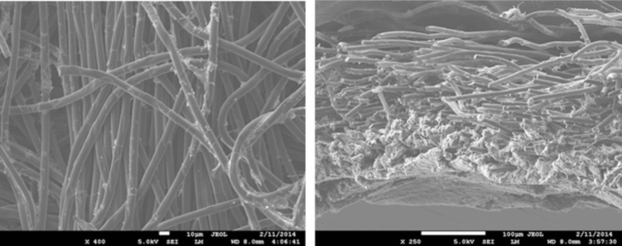
Figure 3. Scanning electron micrograph of (left) GDL surface and (right) DM cross-section with microporous layer on the bottom and GDL on the top.
In this section, we discuss the key approaches toward modeling multiphase flow, especially in DM. Of course, there are always caveats and simplifications that must be made to model the macroscale transport. Thus, the specific pore structure is often considered only in a statistical sense, local equilibrium among phases is often assumed, and the effective properties, which are often measured for the entire layer, are applied locally and assumed to remain valid. We will however discuss some more microscopic modeling and how one can reconstruct PEFC porous media computationally. Next, we explore recent work on issues related to specific interfacial phenomena, contact resistances, and correlating the channel conditions to the droplets and water removal. Such effects could dominate the overall response of the cell and serve as boundary conditions or even as discrete interphase regions. Finally, multiphase flow also encompasses water freezing and melting, and the kinetics of such processes are reviewed.
Incorporation of multiphase phenomena
Modeling the PEFC porous media requires descriptions of the fluxes in the gas and liquid phases, interrelationships among those phases, as well as electron and heat transport. Traditional equations including Stefan-Maxwell diffusion (equation 18), Darcy's law for momentum (equation 42), and Ohm's law for electron conduction (equation 32) are typically used, where most of the effective transport properties of the various layers have been measured experimentally,37 or perhaps modeled by microscopic methods. Effective properties are required to account for the microscopic heterogeneity of the porous structures. This is accomplished by volume averaging all the relevant properties and system variables for transport within the porous domain,
![Equation ([70])](https://content.cld.iop.org/journals/1945-7111/161/12/F1254/revision1/jes_161_12_F1254eqn70.jpg)
where ψk represents any property in the phase k and εk and τk are the porosity and tortuosity of phase k, respectively. As an example, the effective gas-phase diffusivities are both a function of the bulk porosity, εo, and the saturation, S, or the liquid volume fraction of the pore space,
![Equation ([71])](https://content.cld.iop.org/journals/1945-7111/161/12/F1254/revision1/jes_161_12_F1254eqn71.jpg)
The power-law exponents have been shown to have values of around 3 for typical fibrous GDLs,41,42,44,145
![Equation ([72])](https://content.cld.iop.org/journals/1945-7111/161/12/F1254/revision1/jes_161_12_F1254eqn72.jpg)
and are anisotropic with the in-plane value being several times larger than the through-plane one, which also agrees with microscopic modeling results.146,147
For the bulk movement and convection of the gas phase, Darcy's law and the mass-averaged velocity (equations 42 and 13, respectively) are used with an effective permeability that is comprised of the absolute (measured) permeability and a relative permeability owing to the impact of liquid
![Equation ([73])](https://content.cld.iop.org/journals/1945-7111/161/12/F1254/revision1/jes_161_12_F1254eqn73.jpg)
where kr,k is the relative permeability for phase k and is often given by a power-law dependence on the saturation.42,148 The above equations are used along with the mass balance (equation 10) to describe the gas-phase transport.
While one can treat the liquid water as a mist or fog flow (i.e., it has a defined volume fraction but moves with the same superficial velocity of the gas), it is more appropriate to use separate equations for the liquid. This treatment is often of the form of Darcy's law (equation 42), which, in flux form is
![Equation ([74])](https://content.cld.iop.org/journals/1945-7111/161/12/F1254/revision1/jes_161_12_F1254eqn74.jpg)
where  is the molar volume of water. One can also add a second derivative to the above equation such that a no-slip condition can be met at the pore surfaces (i.e., Brinkman equation).149
In terms of heat transport, for DM, the thermal balance turns mainly into heat conduction due to the high thermal conductivity compared to convective fluxes. Although no electrochemical reactions are occurring within the DM, there are still phase-change reactions that can consume/generate a considerable amount of heat, e.g.,
![Equation ([75])](https://content.cld.iop.org/journals/1945-7111/161/12/F1254/revision1/jes_161_12_F1254eqn75.jpg)
where kevap is the reaction rate constant. In typical PEFC porous media, the area between the phases (aG,L) and the reaction rate constant are normally assumed sufficiently high that one can use equilibrium between the liquid and vapor phases. The reaction source terms must be included in the overall heat balance (equation 51), and it should be noted that effective properties are again required to be used in the governing equation, where recent studies have shown the dependence of the anisotropic effective thermal conductivity on water saturation.349,350,105 One must also be aware of contact resistances and interfacial issues to determine the boundary conditions as discussed in the next section.
Finally, there are also modeling methodologies that assume equilibrium among the gas and liquid phases and try to recast the transport equations in order to be computationally more efficient or to converge easier; a prime example is the multiphase mixture model.150,151 In this analysis, although both liquid and vapor phases move simultaneously, they move at different velocities. This difference leads to a drag on either phase. The liquid-phase velocity can be calculated using
![Equation ([76])](https://content.cld.iop.org/journals/1945-7111/161/12/F1254/revision1/jes_161_12_F1254eqn76.jpg)
where the subscript m stands for the mixture, ρk and νk are the density and kinematic viscosity of phase k, respectively, and λL is the relative mobility of the liquid phase which is defined as,
![Equation ([77])](https://content.cld.iop.org/journals/1945-7111/161/12/F1254/revision1/jes_161_12_F1254eqn77.jpg)
A similar equation can be derived for the gas-phase velocity, which is then used to calculate the pressure drop in the gas phase while the Stefan-Maxwell equations 18 govern the diffusive transport of the gas species. In equation 76, the first term represents a convection term, and the second comes from a mass flux of water that can be broken down as flow due to capillary phenomena and flow due to interfacial drag between the phases. The velocity of the mixture is basically determined from Darcy's law using the properties of the mixture. While the use of the multiphase-mixture model does speed computational time and decreases computational cost, problems can arise if the equations are not averaged correctly. In addition, it does not track interfaces rigorously and is typically not seen as a net benefit for most PEFC models since they are not limited computationally, with an exception perhaps being 3-D models.
Liquid/vapor/heat interactions
Equations 74, 71, and 73 clearly show that there is an impact of the liquid- and gas-phase volume fractions on the transport of each other through the various effective transport properties. The key in calculating these relationships is determining an expression for the way in which the saturation varies with the independent driving force, namely pressure. From a continuum perspective, in a capillary-dominated system, these are related through the capillary pressure,98,99,152,153
![Equation ([78])](https://content.cld.iop.org/journals/1945-7111/161/12/F1254/revision1/jes_161_12_F1254eqn78.jpg)
where γ is the surface tension of water, r is the pore radius, and θ is the internal contact angle that a drop of water forms with a solid. This definition is based on how liquid water wets the material; hence, for a hydrophilic pore, the contact angle is 0° ⩽ θ < 90°, and, for a hydrophobic one, it is 90° < θ ⩽ 180°. The capillary pressure can also impact the saturation vapor pressure, which should be corrected for pore effects by the Kelvin equation,
![Equation ([79])](https://content.cld.iop.org/journals/1945-7111/161/12/F1254/revision1/jes_161_12_F1254eqn79.jpg)
where pvap0, o is the uncorrected (planar) vapor pressure of water and is a function of temperature
The functional form of the saturation dependence on capillary pressure can be measured154–159 or derived using various simplistic models141 or more complicated pore-network and other models as discussed in the next section. Figure 4 displays exemplary capillary-pressure – saturation relationships. From the figure, one sees that addition of a hydrophobic (i.e., Teflon) treatment causes the curve to shift toward higher capillary pressures (i.e., more hydrophobic). Also, the gas-diffusion layer exhibits an intermediate wettability where there is a hysteresis between imbibition and drainage that spans pC = 0. However, this hysteresis is not as important since PEFCs operate on the imbibition curve during operation (unless drying is being done) since water is always being injected from the catalyst layer to the gas channel. Similarly, the full curve is not expected to occur because the high permeability of traditional gas-diffusion layers means that once breakthrough and a dominant pore pathway has formed, it is sufficient for removing the liquid water assuming that the ribs do not block too much of the exit pathway. Also shown in the figure is a curve for a catalyst layer, which, due to its small pores, has a wider range of pressures. It is also measured to be more hydrophilic than a GDL, especially if it contains cracks.157
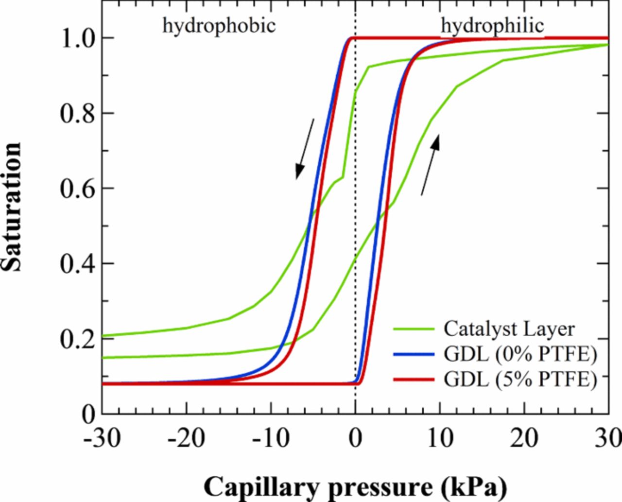
Figure 4. Capillary-pressure – saturation relationships for a crack-free catalyst layer,157 and two SGL GDLs with 0 (blue) and 5 wt-% (red) Teflon.
For use in models, the measured capillary-pressure – saturation relationship is often fit to a function (e.g., hyperbolic tangent) or to a Leverett J-function,146,153
![Equation ([80])](https://content.cld.iop.org/journals/1945-7111/161/12/F1254/revision1/jes_161_12_F1254eqn80.jpg)
However, such a treatment is not rigorously defined for fibrous media and it has limited applicability in terms of predictability in terms of the properties in the above equation.
A somewhat less empirical way to treat the capillary-pressure data in that it is not solely a curve fit is to describe the curve using the separately measured pore-size distribution and a contact-angle distribution141
![Equation ([81])](https://content.cld.iop.org/journals/1945-7111/161/12/F1254/revision1/jes_161_12_F1254eqn81.jpg)
where ro,k and sk are the characteristic pore size and spread of distribution k, respectively, and fr, k is the fraction of the total distribution made up of distribution k, where the fr, k's sum to unity. The contact-angle distribution, which is a measure of the surface energies encountered by liquid water within the pores, is given by
![Equation ([82])](https://content.cld.iop.org/journals/1945-7111/161/12/F1254/revision1/jes_161_12_F1254eqn82.jpg)
where θo,n and σn are the characteristic contact angle and deviation of distribution n. The integration in equation 81 is done with respect to the critical radius as determined from equation 78,
![Equation ([83])](https://content.cld.iop.org/journals/1945-7111/161/12/F1254/revision1/jes_161_12_F1254eqn83.jpg)
which is a function of hydrophobicity and thus the integral is separated into terms representing hydrophobic and hydrophilic contact angles since the critical angle approaches infinity at a zero capillary pressure. Finally, one can also incorporate the residual saturation, Sr, as shown in Figure 4
![Equation ([84])](https://content.cld.iop.org/journals/1945-7111/161/12/F1254/revision1/jes_161_12_F1254eqn84.jpg)
Using the above integration approach, one can also determine expressions for the relative permeability of the liquid and gas of
![Equation ([85])](https://content.cld.iop.org/journals/1945-7111/161/12/F1254/revision1/jes_161_12_F1254eqn85.jpg)
and
![Equation ([86])](https://content.cld.iop.org/journals/1945-7111/161/12/F1254/revision1/jes_161_12_F1254eqn86.jpg)
respectively, where fHI is given by
![Equation ([87])](https://content.cld.iop.org/journals/1945-7111/161/12/F1254/revision1/jes_161_12_F1254eqn87.jpg)
and an effective saturation is used for the liquid relative permeability
![Equation ([88])](https://content.cld.iop.org/journals/1945-7111/161/12/F1254/revision1/jes_161_12_F1254eqn88.jpg)
This treatment is not as rigorous as more complicated microscopic models as it assumes a cut-and-join bundle of pores, but also it does not require the complexity and cost of more microscopic treatments.
The above discussion is based on assuming that one can weight the liquid and vapor transport through the phase volume fractions. In addition, when used in macroscopic models, the underlying assumption is that the capillary-pressure – saturation relationship can be applied locally although it is measured or typically predicted for the entire layer. The validity of this assumption still remains an open question, especially since it is known that DM structures are not spatially homogeneous.
Although the liquid and gas phases are related through transport properties, they also have an effect on each other's fluxes through heat transport and phase-change-induced (PCI) flow.29,160,161 In this fashion, the liquid water is near equilibrated with water vapor and the temperature distribution induces a water vapor-pressure gradient. The water is transported along that gradient and condenses and gives off heat at the gas channel or cooler flowfield rib as shown in Figure 5. Such an effect can be shown to be able to move all of the produced water when operating above temperatures of 60°C or so with typical component properties.160 In this fashion, the produced water is transported through the cell components in the vapor phase and flooding concerns will be minimal and result mainly from condensation in the flowfield channels or at the GDL / flowfield- land interface. Thus, PCI flow is the dominant mode of water removal at higher temperatures, and may even cause the cell water content to decrease at higher current densities because the heat generated outpaces the water generation. However, while the water-removal characteristics are a benefit of PCI flow, the net flux of water vapor is now out of the cell, which can results in the gas-phase velocity also being out of the cell (see equation 13). In either case, the movement of the water vapor from the catalyst layer to the gas channel due to PCI flow represents a mass-transfer limitation in terms of getting oxygen to the catalyst layer since it now must diffuse against that flux. Finally, PCI flow also results in substantial heat removal from the hotter catalyst layer, thereby flattening the temperature gradients.
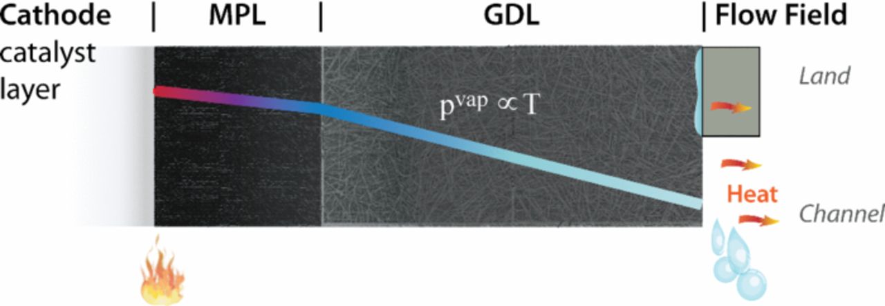
Figure 5. Schematic representation of phase-change-induced (PCI) flow.
Ice formation
In the preceding section, we focused on multiphase aspects in terms of liquid and vapor. However, in both automotive and stationary applications, PEFCs must permit rapid startup with minimal energy from subfreezing temperatures (i.e., cold-start), where water can solidify to form ice in the MEA. This freezing can severely inhibit cell performance and often results in cell failure.162–166 In recent years, several cold-start targets have been established by the Department of Energy.167 Two key targets are that the PEFC must be able to start unassisted from –40°C, and reach 50% net power within 30 s from –20°C. Despite significant attention, successful cold-start from T < −20°C remains a challenge.167 Achieving such a startup is difficult in practice due to potential flooding, sluggish reaction kinetics, durability loss, and importantly, rapid ice crystallization that is counteracted by the heating of the cell due to the reaction waste heat and ohmic heating.168 Typically, the cell potential decays rapidly at low temperatures and/or high current densities due to ice formation at the reactive area of the cathode.162–166,169,170 The traditional method to provide successful cold-start is to purge the system of water on shutdown, thus providing a sink in the membrane for the water production during startup and allowing for the heating of the stack before irreversible flooding and ice formation occur. Such a strategy seems to work above − 20°C, but not at lower temperatures, due to issues discussed below; in addition, one prefers to develop and understand a possible optimal and material solution to cold-start.
Over the past decade, several numerical continuum cold-start models have been developed.162,163,170–175 To counter the difficulties associated with cold-start, models emphasize both procedural strategies and materials design. For example, Balliet et al.162,171 recommend higher potentials during startup to optimize performance from –20°C as well as increased water capacity or reservoirs (e.g., increased porosity). Numerous studies have also examined the stack-level thermal response during cold-start.81,164,174 However, relatively few studies model the water and ice within the PEFC.163,164,171,174 Early models assume that product water vapor instantaneously solidifies when the vapor partial pressure exceeds the saturation value.81,164 As a result, they do not account for liquid water explicitly within the PEFC.
More recently, Jiao et al.174 and Balliet et al.162,171 extended cold-start models to include vapor, liquid, and solid phases of water within the PEFC. The equilibrium freezing point of ice within the GDL, catalyst layers, and PEM is based on a characteristic pore size using the thermodynamic Gibbs-Thomson equation,176
![Equation ([89])](https://content.cld.iop.org/journals/1945-7111/161/12/F1254/revision1/jes_161_12_F1254eqn89.jpg)
where TFPD is the amount of freezing-point depression,  is the molar volume of ice, γ is the surface tension of the ice-liquid interface, Tm is the melting (freezing) temperature for bulk water, ΔHf is the heat of fusion of ice, and r is the pore radius. The amount of freezing-point depression in a given pore is primarily a function of pore radius – smaller pores tend to freeze at a lower temperature due to the shift in w chemical potential. Because real media have distributions of pore radii, the fraction of unfrozen water versus temperature is generally a continuum below 0°C. The overall rate of ice formation is then expressed as a linear rate equation
![Equation ([90])](https://content.cld.iop.org/journals/1945-7111/161/12/F1254/revision1/jes_161_12_F1254eqn90.jpg)
where the equilibrium liquid saturation, SL(TFPD), is a function of pore properties and is derived from a thermodynamic relationship.82,177
This thermodynamic-based freezing circumvents the use of ice-crystallization rate expressions, since at the time, none were available for PEFC-porous media. Furthermore, in recent years, in-situ visualization and detection of ice formation within PEFC-porous media has progressed.166,178–180 In all cases, generated water was observed initially in the subcooled state, particularly between –2 and –20°C. Although water did not freeze immediately, the mechanisms and kinetics of ice crystallization were not investigated.
Recently, Dursch et al. measured the kinetics of ice nucleation and growth in traditional GDLs and catalyst layers using differential scanning calorimetry.163,181,182 They demonstrated that the kinetic-based approach shows a significant departure from the commonly-used Gibbs-Thomson equation due to the impact of kinetics (i.e., assuming instantaneous thermodynamic equilibrium is not valid). In all cases, ice crystallization was preceded by a limiting stochastic induction time, τi, that depends strongly on both temperature and material properties.163,181,182 From these kinetic data, they developed validated ice-crystallization rate expressions to aid numerical continuum cold-start models. The rate expressions are based on the Johnson-Mehl-Avrami-Kolmogorov (JMAK) formalism163,181,182
![Equation ([91])](https://content.cld.iop.org/journals/1945-7111/161/12/F1254/revision1/jes_161_12_F1254eqn91.jpg)
with
![Equation ([92])](https://content.cld.iop.org/journals/1945-7111/161/12/F1254/revision1/jes_161_12_F1254eqn92.jpg)
where  is the number-average crystallization temperature, ϕ is gas-free volume fraction of ice within the pores defined by ϕ ≡ SI/(SI + SL), αL is liquid thermal diffusivity, ηo(T) is a dimensionless temperature-dependent growth parameter (see Equation 9 of Dursch et al.),181 θ is the contact angle of the ice/water/substrate triple line, g(θ) = (2 + cos θ)(1 − cos θ)2/4 for heterogeneous nucleus growth on a flat surface, and J(T) is the pseudo-steady-state nucleation rate (nuclei m−3 s−1) that has a form based on classical-nucleation theory of193,198
![Equation ([93])](https://content.cld.iop.org/journals/1945-7111/161/12/F1254/revision1/jes_161_12_F1254eqn93.jpg)
where A and B are determined empirically and Tref is taken to be the temperature of liquid-water freezing under standard conditions (273.15 K). The values of J(T) can be measured by repeated experimental freezing studies.163,181,182 Finally, to obtain  , the definition suggested by Kaschiev183 is adopted
![Equation ([94])](https://content.cld.iop.org/journals/1945-7111/161/12/F1254/revision1/jes_161_12_F1254eqn94.jpg)
where Vo is liquid volume of a water-saturated PEFC porous medium.
To validate ice-crystallization kinetics within PEFCs, Dursch et al. compared measured to predicted MEA cell-failure time in a simplified isothermal kinetic cold-start model.163 Figure 6 compares predicted to measured (symbols) tfail versus subcooling, ΔT = Tref − T, defined as the magnitude of the difference in the temperature of freezing and 273 K. Solid and dashed lines correspond to the kinetic-based approach163 and thermodynamic-based approach (equation 90),171 respectively. As subcooling extends beyond ΔT = 11 K, ice-crystallization kinetics is well approximated by the thermodynamic-based approach, since ice crystallization occurs rapidly. However, in the kinetic approach, the particular ΔT that establishes the "nucleation-limited" regime relies heavily on all heat-transfer and kinetic parameters. Accordingly, these controlling parameters can be adjusted to significantly delay or even prevent ice formation. The impact of the nucleation-limited regime is also shown to agree better with experimental isothermal cold-start data, and the other experimental findings mentioned above.
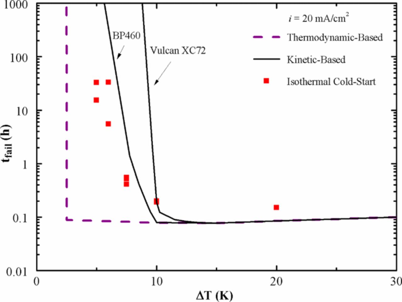
Figure 6. MEA-cell-failure time, tfail, for isothermal galvanostatic start-up as a function of subcooling at a current density of 20 mA/cm2 (figure reprinted from Reference 163 with the kind permission of the publisher).
In addition to freeze kinetics, Dursch et al.184 also examined non-isothermal melting in the GDL. It was shown that ice-melting times decrease nonlinearly with increasing heating rate, although the melting temperatures remain at the thermodynamic-based values (consistent with Gibbs-Thomson, equation 89) but are rate limited by heat transfer. Using a moving-boundary Stefan problem, they derived an expression for the melting time,
![Equation ([95])](https://content.cld.iop.org/journals/1945-7111/161/12/F1254/revision1/jes_161_12_F1254eqn95.jpg)
where L denotes bulk-ice or GDL thickness, ρL is liquid mass density,  is latent heat of fusion per unit mass of ice (taken as positive), U is the overall heat-transfer coefficient, β is the heating rate (K/min), and the other variables are as already defined. This melting time should be incorporated into cold-start simulations.
Microscale modeling and reconstruction
Within the area of numerical simulation for the performance and durability of PEFCs, there has always been a great interest and need to understand the linkage between the properties of the component materials in the MEA and the performance of the unit cell and stack. As research progressed and an increasing level of detail was paid to the fabrication, engineering, and effect of the individual component properties on the overall PEFC performance and durability, there began to emerge attempts to resolve the morphology of the components with ever increasing levels of resolution and detail. These morphology-based simulations are typically ascribed with the label of being microstructural simulations and are related significantly to transport and multiphase aspects.
For each component within a PEFC, a relevant length scale can be considered dependent on the physical process being considered and the morphology of the component itself. In regards to this, one typically finds that the analysis of the PEFC porous media (i.e., GDLs, MPLs, catalyst layers) are accomplished using similar methodologies, while analysis of the polymeric membrane, for example, has traditionally lent itself more toward the application of molecular dynamics-based approaches. While the latter is outside the scope of this review, some remarks should be made on the former. Morphological-based models offer the potential to investigate explicitly the relationship between the porous media and the specific transport property generally with consideration given for the constituent material properties, spatial distributions, and statistical variations that may originate within manufacturing processes. In order to make these linkages, however, a virtual method of representation of the component structure is required.
Porous media within PEFCs are generally accepted to fall into the category of random, heterogeneous porous media. It was from the aerospace, metallurgy, and energy industries that some of the earliest attempts at morphological analysis and numerical reconstructions are found.185,186 Typically, there are two main methodologies employed in generating a virtual morphology with the first being a stochastic-based reconstruction method in which a statistical distributions, randomness, and a series of rule-sets are used as a basis to create a "representative" morphology. The second method, image-based reconstruction, employs experimental diagnostic imaging, such as SEM, TEM, or X-ray computed tomography (XCT), combined with a numerical processing step that converts the images to a virtual structure thus translating the original experimental images into a morphology that can be used for numerical analysis.187–190
For the latter approach, this can be accomplished, for example, by extracting images from the center lines of single fiber from the resultant images of GDLs. These center lines are then used in conjunction with a stochastic algorithm to reconnect parts of the center lines in an attempt to preserve the curvature of the fibers.190 The limitation of the rendered pore space and features within the domain remain the limit of the spatial resolution of the imaging technique itself as well as the ability to determine the distinct phases (e.g., Teflon and carbon and sometimes water are not easy to distinguish with X-rays).191
For stochastic reconstruction, the virtual generation of the microstructures relies on the use of a random number generator, statistical distribution of geometric information relating to the constituent materials that comprise the media, and a series of rule-sets.192–195 Typically these rule-sets are an attempt to impose physical constraints on the placement algorithms in order to make the creation of the domain more tractable, such as constraining fiber size, overlap, interactions, etc.193 The constraints placed on the invariance of domain properties in the non-through-thickness directions are directly related to the overall numerical intensity of the final simulations as constraining the morphological model to as small a sample as possible dramatically increases the speed of the simulations. However, the main criteria in deciding this aspect should relate primarily to the size of the morphological domain relative to the transport coefficient of interest, wherein the transport coefficient does not vary if the domain size changes (i.e., it is a representative volume element). An example of a reconstruction of a GDL is shown in Figure 7, where one clearly observes the fibrous structure.196
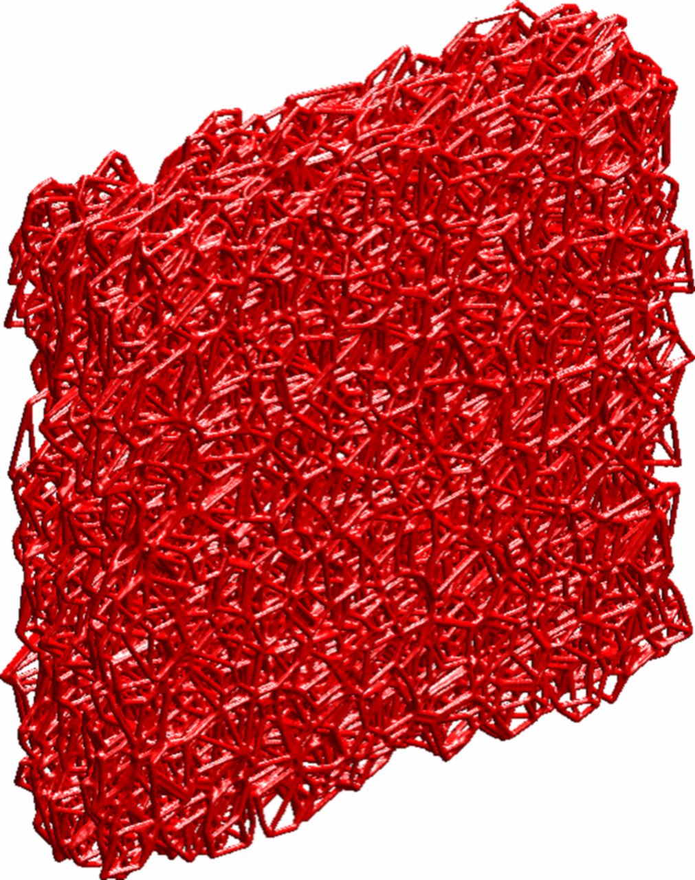
Figure 7. Schematic of a computationally reconstructed carbon-fiber paper (reprinted from Ref. 196 with the kind permission of the publisher).
For all of these simulations, it should be noted that predicting a volume-averaged coefficient for use in macroscopic models necessitates conducting simulations enough times to get representative structures and values. Thus, the use of a quality random number generator is paramount in generating an appropriate numerical representation, where it has been suggested that the use of 25 samples is sufficient to represent an appropriate sample set given the stochastic nature of the experimental geometry data.197 The need for the larger sample set is especially the case since validation of the microstructures by imaging and other methods (e.g., porosimetry) are typically through general, statistical information,198 of which various microstructures may still agree with the data. Ultimately, it is best to compare aspects that relate directly to the distribution of material through the sample but on a statistical or probabilistic basis, thus the use of both imaging and measurable characteristics are ideal.
Due to the increasing amount of structural characterization and the virtual microstructures, it is now possible to model transport through the DM using direct simulations.188,194,199,200 These models can provide the critical effective properties needed for the cell-level models, however, they require detailed information on internal surfaces and chemical information (e.g., wettability), which, as described above, is not always readily available. In addition, they are still numerically intense (especially for the statistical number of simulations required). For example, Zamel et al. discuss that the mesh in their simulations ranges from 135,000 to 2.3 million grid points with the number depending on the total porosity of the structure.194 Similarly, Lattice-Boltzmann methods may likewise be used but require the same kind of detailed chemical and structural information as well as knowledge of the underlying forces acting on and between the various fluids and components.201–211 They have also been shown to not necessarily provide significantly more insight than the simpler pore-network approaches, especially for use in macroscopic simulations and with typical GDL saturations around 0.1 to 0.3.212 A detailed description of such methods is beyond the scope of this review due to the above mentioned issues.
A large amount of research and analysis has been done to improve the capability in the morphological modeling area in the last decade. Domain generation has become sufficiently more sophisticated with techniques being developed to generate stochastically not just fiber arrangements but full DM structures including Teflon, binder, and MPLs.213 Thus, such models are valuable areas for continued research and development. In addition, experimental techniques in terms of characterization of the various effective properties are also increasing in scope and complexity as discussed in a later section. However, as mentioned in the previous section, most of these experiments remain valid for only the entire layer, and not as a function of DM thickness. Thus, to be used in situations where there are gradients and flow, one needs to assume local equilibrium and that a given volume element is representative of the entire domain; such an assumption remains unproven. Overall, there is a need to understand the physics within the DM but without necessitating the determination of a substantial set of unknown parameters.
Pore-network modeling
A promising treatment that satisfies those requirements is that of pore-network modeling.98,99 Such an approach allows one to model the pore-length scale, and therefore account for the capillary-driven processes, thermal processes, and water distribution. However, it is still too computationally costly to account for all of the coupled physics along with the rest of cell components. Therefore, it is valuable for use in a multiscaling approach wherein the pore-scale models yield the functional relationships required for the more macroscopic complete-cell models (e.g., saturation, effective properties, etc.). Pore-network modeling allows for consideration of more physical and chemical properties than the macroscopic approaches described in the preceding section.
A pore-network model utilizes a simplified description of the pore space within the DM. Thus, one idealizes the geometry in terms of pores and interconnections (nodes) as shown in Figure 8.146,196,214 The throat lengths and sizes are taken from analysis of either theoretical or actual (e.g., XCT)188,215–218 images of the DM that are digitized and analyzed using methods and approaches mentioned above in the previous section. It should be noted that although the network implicitly assumes cylindrical pores, in reality it is a resistor network wherein the actual non-cylindrical pores are casted in terms of effective cylindrical ones that have the same resulting resistance toward transport,196 and a similar effective resistance can also account for changes in surface interactions (e.g., wettability) although this is less well known and utilized. The generated network is validated by comparison of calculated and measured parameters including the pore- and throat-size distribution data as well as measurements such as the capillary pressure – saturation relationship. Water flow and distribution within the generated network (Figure 8) is solved by a stepwise fashion from one point to another, and thus is independent of the real-space discretization grid (i.e., it only depends on the network).
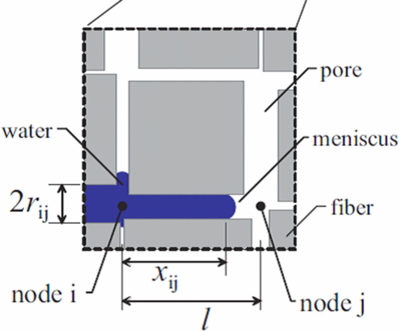
Figure 8. Schematic of a pore-network-model solution (figure reprinted from Ref. 214 with the kind permission of the publisher).
For modeling transport, the same governing equation and multi-phase phenomena described in the above sections remain valid. For example, for liquid-water imbibition, the model examines each intersection or node where the water travels based on the local pressure and pore properties. The volumetric flowrate of water in a cylindrical pore of radius rij between nodes i and j (see Figure 8) is governed by Poiseuille flow
![Equation ([96])](https://content.cld.iop.org/journals/1945-7111/161/12/F1254/revision1/jes_161_12_F1254eqn96.jpg)
where Δpij is the pressure acting across the pore, l is the pore length, and  is the capillary pressure in the pore when multiple phases are present. The volumetric flowrate exists only when
  . The effective viscosity within a pore, μeffij is a function of the fluid position inside the pore, xi,j, the non-wetting (injected) fluid viscosity, μnw, and the wetting (displaced) fluid viscosity, μw. The effective viscosity is modeled to provide a smooth transition between the wetting and non-wetting viscosities while a pore is neither completely filled nor empty. The capillary pressure is also modeled as a function of the fluid position within each pore. It is calculated similar to equation 78 but where either the average radius of the intersecting pores at each node or the radius of a given pore is used depending on where the water meniscus exists,
![Equation ([97])](https://content.cld.iop.org/journals/1945-7111/161/12/F1254/revision1/jes_161_12_F1254eqn97.jpg)
where  and
and  are the average pore radius around node i and j, respectively, The capillary pressure is zero when the pore is filled with only one fluid. Conservation of mass requires that the flowrate balance at each node for every simulation step, thus from equation 96 one gets
![Equation ([98])](https://content.cld.iop.org/journals/1945-7111/161/12/F1254/revision1/jes_161_12_F1254eqn98.jpg)
where the summation is over all of the pores connecting to the node (normally 4). The unknown pressure gradient, Δpij, is solved through the equation above. In addition to the pore sizes and lengths, one also needs the pore contact angle and fluid properties.
A sample output of a pore-network model is shown in Figure 9.214 As can be seen, the model can show the distribution of the water, and in the top figure one can see that a dominant pore pathway has formed. The simulations are stochastic, similar to the transport of water in the DM, and thus enough realizations are required for understanding as discussed above. Such distributions can also provide direct insight and help in terms of understanding the impact of the water network on the exterior interfaces as discussed in sections below. The distributions can then be used in other transport simulations to predict the gas-phase tortuosity and effective diffusion coefficients, which are needed for the macroscopic modeling of the gas phase. Currently, the pore-network models do not yet contain all of the physics, although advancements such as including phase change and coupled thermal effects are providing promising results. Work is also needed in understanding and incorporating thickness-dependent structural heterogeneities and in linking these models with boundary conditions defined by interfacial interactions with the other PEFC components.
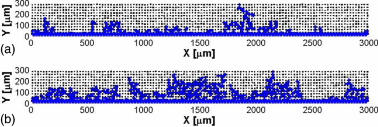
Figure 9. Water distributions at the time a capillary finger reaches the gas flow channel for two pore networks generated from the same pore-size distribution (figure reprinted from Ref. 214 with the kind permission of the publisher).
Interfaces
The impact of interfacial regions in the PEFC has so far been commonly neglected in classical full-cell multiphase modeling efforts. Traditionally, the interface between two layers or the channel wall and DM has been neglected or simply treated as an infinitely thin barrier with discrete property values on either side and no co-mingling of surfaces and properties. However, more recent modeling and experimental work has demonstrated the importance of these interfaces in water storage, transport, and durability. Also, the interfacial conditions typically drive the transport phenomena and are key in determining the boundary conditions for the various models. The specific interfaces of interest discussed in this section include the DM with the catalyst layer, the boundary between the MPL and GDL, and the interactions and interface between the GDL and flowfield, which could be critical in terms of setting the lower value of the liquid pressure and thus holdup within the cell.
Classical macroscopic models only consider a bulk contact angle, pore size, tortuosity, porosity, and thermal conductivity in calculation of liquid transport with bulk capillary-transport functions,219 and neglect any interfacial regions, or capillary action formed by the channel wall interface with the diffusion medium. However, one expects that the performance is quite different when the interfacial conditions above are changed, even if the normal multiphase parameters listed are identical. Clearly, there is much more to study in order to develop the next-generation of optimized materials and designs with advanced multiphase models incorporating these effects.
Membrane / catalyst layer
The membrane / catalyst layer interface is often overlooked. In fact, only a few models assume non-equilibrium95–97 even though, as mentioned there is thought to be an interfacial resistance toward at least water-vapor transport51–68,92,93 and assumingly transport of other species as well. Through-plane conductivity results are inconclusive since those done in vapor normally require a correction for interfacial contact resistance220 (which can mask any interfacial resistance), and in liquid one does not observe an interfacial resistance.54,62,67 The thought is that the morphology of the interface may change depending on its environmental contact.50–67,89,90
However, this contact is confused in the case of the catalyst layer with the membrane since the membrane may be in contact with liquid, vapor, and/or catalyst-layer ionomer. Thus, the question then is how to treat such a complex interface. Typically, one assumes a seamless boundary between the membrane and catalyst-layer ionomer in terms of ionic flux and conditions; however, there are a couple of issues with this treatment. First, as discussed in a later section, even for the same conditions, the water content in the catalyst-layer ionomer is different than that in the membrane due to confinement, and thus one is unsure what to equate (e.g., activity, water content, etc.), especially since there may be transport between the confined and unconfined (i.e., membrane) domains due to removal of the confinement. Second, this treatment assumes rapid in-plane transport in the membrane and no direct influence of the environment outside the membrane. In his thesis, Meyers221 demonstrated that a membrane partially submerged in liquid has an average water content between that of vapor and liquid, thereby demonstrating such an assumption of rapid in-plane transport is not necessarily valid. In addition, the model of Weber and Newman50 had to be adjusted to a phase-in-contact approach, where the membrane water content is taken to be the average between that expected due to the contacting phase volume fractions at the membrane / catalyst-layer interface, in order to match experimentally measured water-content values.66 In terms of transport, Adachi et al.222 demonstrated that across the membrane the transport seems to be dominated by the liquid-equilibrated mode when both liquid and vapor exist, although this is not necessarily unexpected since the liquid-transport coefficients are significantly larger than the vapor ones; therefore, any transport in parallel would be dominated by the liquid-equilibrated transport mechanism.
Finally, many catalyst layers often contain ionomers that are different in structure or equivalent weight than that of the membrane since, within the catalyst layer, the ionomer must transport oxygen as well as protons and does not require as much mechanical stability. Such an interface between two different ionomers may cause a mismatch in properties (e.g., electro-osmotic coefficient) and interfacial phenomena that could result in transport issues.223 The above discussion demonstrates that the membrane / catalyst-layer interface and its treatment is still unknown and worth further research. It should be noted that both the anode and cathode membrane interfaces are critical, especially as the anode has a sharp reaction distribution typically at this interface.224
Catalyst layer/microporous layer
The vast majority of literature treats the catalyst layer / MPL interface as a perfectly mated, parallel interface. The reality is, however, that the two mating surfaces are not perfectly smooth or straight as shown in Figure 10, and a mismatch between the elasticity and surface roughness of the interfaces results in small gaps and non-contact zones between the two surfaces, even under elastic compression.225 Additionally, in conventional channel/land architectures, the transmitted compression pressure under the channels is much less than under the lands, which can also result in a different interface compression condition. The net effect of this interfacial roughness mismatch between the MPL and catalyst layer is a zone of imperfect contact with microscopic gaps as shown in Figure 11. Figure 11b was formulated by application of a compressed-surface-interaction model and experimental topographical scans of a commercial MPL and catalyst surface.226 Based on these findings,225–231 the potential interfacial gap storage volume can be significant, and depends directly on the elasticity, smoothness of the mating surface (and if there is a mismatch in roughness) and compression pressure. Thus, the worst condition is under a channel with near zero overburden (compression) pressure, with a cracked, stiff MPL with much greater surface roughness than the catalyst layer. Under these conditions, the local gaps at the catalyst layer / MPL interface can be significant and can impact the transport phenomena in the cell.
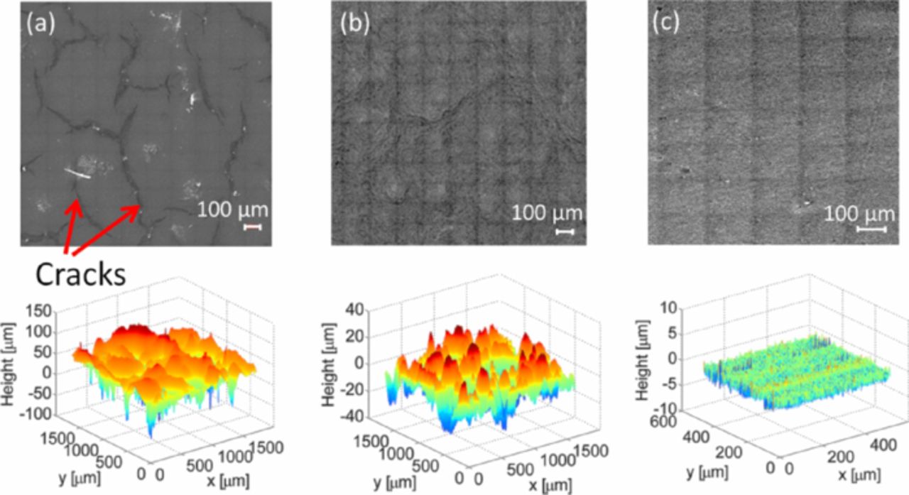
Figure 10. Optical micrographs and 3D surface heights for a) MPL with cracks, b) MPL without cracks and c) CL (images reprinted from Ref. 228 with the kind permission of the publisher).
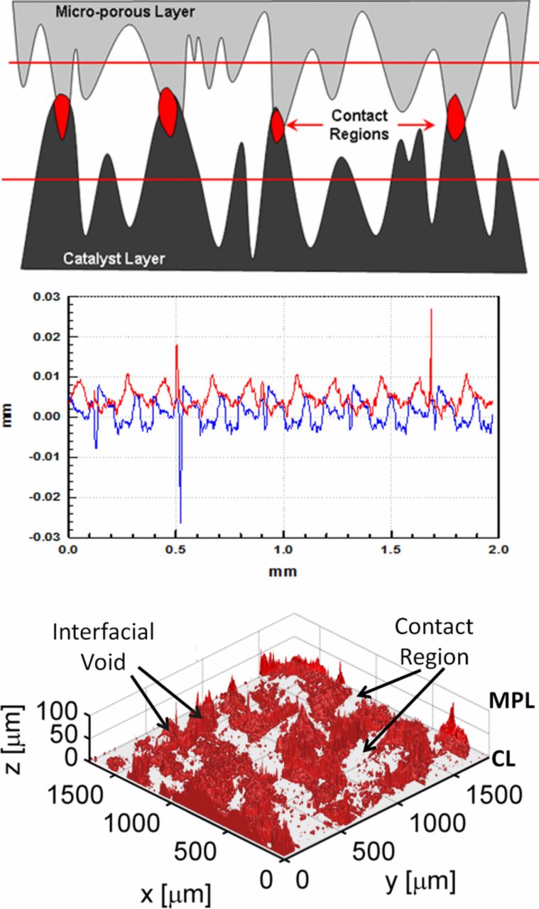
The additional gaps created between the surfaces will affect the electronic transport across the interfaces. However, unless the gaps are exceptionally large, there will be no significant impact on the measured performance due to ohmic losses between a mismatched and well-matched interface. The key controlling parameters in the presence of additional losses caused by a gap are the in-plane conductivity of the mating layers, the width of the gap, and thickness of the interface. Bajpai et al.227 computed losses along the MPL interface as a function of gap width and thickness and found that for normal conductivities, ohmic losses are minor until a dimensionless gap width of around 10 (see Figure 12).227,228,230 This dimensionless ratio is also relevant for other modes of transport. Thus, interfacial gaps that would have significant ohmic implications are not likely in a normal catalyst-layer / MPL interface, without some blistering or delamination caused by ice damage or other phenomena.
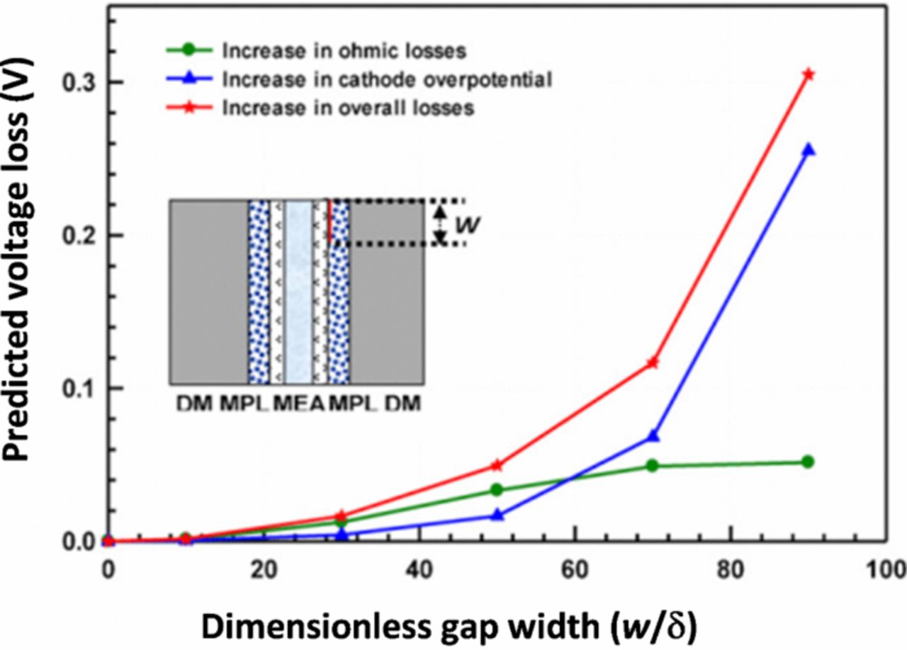
Figure 12. Calculated increase in cathode ohmic and kinetic losses as a function of gap width to thickness ratio in the MPL (image reprinted from Ref. 227 with the kind permission of the publisher).
Similar to ohmic transport, the thermal disruption from the small gaps was calculated to be minimal for normally-distributed surface- roughness-related discontinuities under compression.227,230 Larger disruptions, or low contact pressure, result in local hot spots (if gas filled) or cooler spots (if liquid filled). Small local gaps and interfacial contact gap volumes are locations where liquid-water accumulation is favored due to low local capillary pressure. Thus, these reservoir volumes will fill and pool first and will subsequently be the last to drain or evaporate upon shutdown. Similar to the ohmic and heat-transfer considerations, isolated small volumes of liquid are not predicted to be a major factor in the performance, as the effective gas-phase transport distances around the volume are not significantly larger than the normal path lengths at normal saturation levels. However, as shown in Figure 13, they can contain a non-negligible amount of the total liquid water.230 Of greater importance is the possible existence of a liquid film along the interface, which hinders the gas transport to the catalytic sites. Direct evidence of the presence of water films along the catalyst layer / MPL interface under the channel (where overburden pressure is lower) is shown in Figure 14, in terms of an ice-lens growth following freeze/thaw cycling.232–235 As shown in Figure 14b, the high-frequency resistance of the cell was increased, indicating a significantly large ice lens was present in agreement with the analysis of Figure 12.
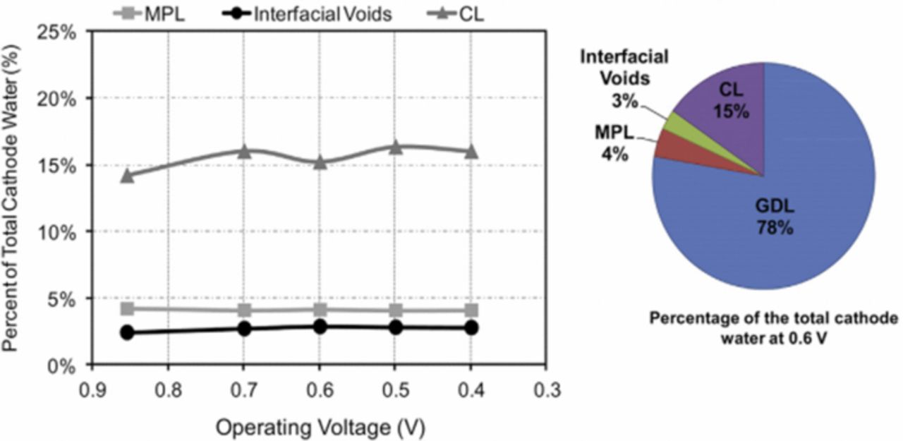
Figure 13. Predicted distribution of liquid water in the cathode, with interfacial voids (image reprinted from Ref. 230 with the kind permission of the publisher).
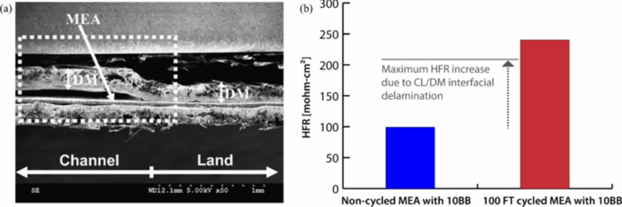
Figure 14. (a) Evidence of interfacial ice lens formation and delamination after 100 freeze-thaw cycles (b) measured high-frequency resistance showing evidence of interfacial delamination impact under extreme conditions (images reprinted from Ref. 233 with the kind permission of the publisher).
As mentioned, the MPL provides specific entry points into the GDL for liquid water; these pathways are nominally formed at cracks. From a gas-phase heat- and mass-transport perspective, these cracks should have little effect. Thus, impact from the cracks is expected to be a result of changes in liquid-water motion and accumulation. Similarly, access of liquid water to the cracks requires sufficient in-plane transport in the catalyst layer or along the heterogeneous interface. Thus, the rough interface may provide for better water removal, but at the detriment of forming a film and blocking gas transport. Similarly, pooling in these gaps can also enhance low RH operation,137,138 but perhaps not higher RH operation if there is liquid condensing in the GDL and trying to move back into the catalyst layer.236 While the engineering of water pathways throughout the whole DM has been investigated experimentally, 237–242 there is a lack of modeling studies. In addition, the tradeoffs of having interfacial gaps and their possible engineering along the interface is something that modeling can, but has yet to, address in a substantial fashion.
Microporous layer / gas-diffusion layer
The boundary between the GDL and MPL is one of the least studied interfaces in a PEFC. Part of the issue is that neutron and other visualization techniques have so far failed to provide the sub-micrometer resolution needed to confirm various modeling approaches. However, it is known that this interface is not sharp (see Figure 3), and has been measured by X-ray tomography to have a standard deviation of more than 20 μm. The classic treatment of this boundary is again as infinitely thin with discrete media with different transport parameters on both sides, especially since the governing equations throughout both domains remain the same. The result of this assumption is the prediction of a "saturation-jump" between the MPL and DM,142,243,244 where the high hydrophobicity of the MPL and small pores results in a very low saturation in this layer that is discontinuous with the larger pore size, lower hydrophobicity GDL. In practice, however, neutron imaging and higher-resolution X-ray imaging has not shown this to be the case,160,245 although due to resolution and imaging limitations as well as the intermixing of the MPL / GDL components, the evidence is not conclusive.
Gas-diffusion layer / flowfield
The GDL / flowfield interface is the most widely studied of the interfaces, especially as it is critical for water management. Several of the effects described above such as PCI flow are directly related to this interface. In addition, the boundary condition at the channel/GDL interface controls much of the water retention in the cell and is of paramount importance in terms of understanding and predicting multiphase flow. This boundary condition is typically a specification of flux or concentration for water vapor and one of saturation or liquid pressure for liquid water. However, if one is using a two-phase model without a residual effective permeability, then setting saturation equal to zero could be problematic in terms of convergence since this condition enforces the fact that all water must leave the GDL in the vapor phase since the effective permeability will go to zero. We believe that it is better to set the liquid pressure or capillary pressure, and ideally this pressure should be associated with the formation and existence of droplets on the GDL surface as described below.
The GDL / flowfield-land interface is of greatest importance in electron246,247 and heat transport,248 as the contact resistance across this boundary can be highest here compared to other interfacial layers. In conventional channel/land architectures, the land is impermeable and is cooler than the GDL/ channel interface due to direct conduction to the flowfield plate. Thus, liquid tends to accumulate under the land by condensation,29,161,249 until removal via in-plane flow or evaporation. Figure 15 illustrates the process of under-land accumulation, followed by flow into the channels via capillary action up the channel walls into droplets if the channel wall is hydrophobic (Figure 15a) or film if hydrophilic (Figure 15b).250 The shape of the interface should also play an important role in the water removal, as a rounded land edge will tend to more efficiently draw water out of the GDL along the channel-wall interface than an abrupt corner will.
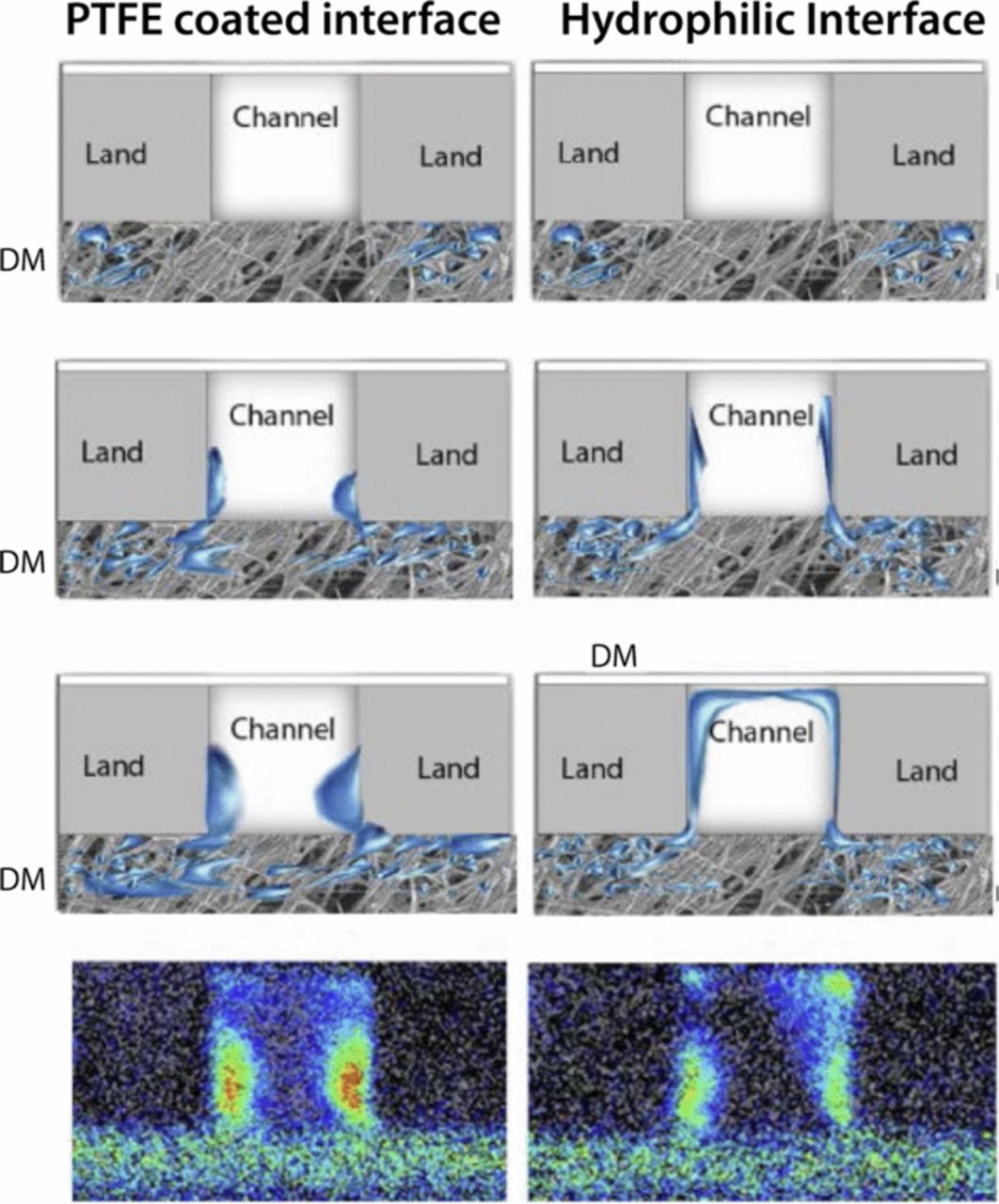
Figure 15. Schematic and neutron image of water accumulation and capillary motion for hydrophobic and hydrophilic channel-wall interfaces (image reprinted from Ref. 250 with the kind permission of the publisher).
The GDL / flowfield-channel interface is important for water management as mentioned, as the gas must enter the GDL and water must be removed. As shown in Figure 14, this can be accomplished through capillary interaction at the lands. Alternatively, liquid water can be removed as droplets in the channel assuming conditions of multiphase flow exist (i.e., 100% RH). Once in the channel, the water moves either along the walls, as a mist, or stochastically by forming films that are periodically removed due to gas-pressure buildup.72,251,252 The key conditions for this boundary condition are being able to predict the surface coverage of water or droplets and the subsequent capillary pressure or liquid pressure as a function of material properties and operating conditions. This is something that has been researched both theoretically and experimentally, but not yet clarified and utilized, especially in PEFC cell modeling.
To understand water-droplet behavior, emergence, and detachment, and to provide more physical basis for modeling the interface, detailed droplet-specific studies have been accomplished.40,251,253–257 These studies have highlighted some of the fundamental issues and have examined liquid-water droplet and water removal from PEFC flowfield channels. It has been shown that droplets form periodically at specific locations and with an associated varying liquid pressure,258,259 which can be related to the breakthrough pressure and then subsequent growth and detachment phases as shown in Figure 16. Analyzing the 110 μm curve, the initial pressure signal is due to head from water traveling through system lines and filling void space between the GDL and injection port. At approximately t = 700 s, a steep climb begins due to water being forced into GDL pores; the slope is attributable to expansion of the injection system. At about t = 1200 s pressure reaches a maximum which is accompanied by droplet formation on the GDL surface. This maximum pressure is the breakthrough pressure, followed by a dramatic fall in signal as the pressure decays to Darcy resistance inside the GDL pores. Subsequent runs will then show a smaller rise between the breakthrough and Darcy pressures. This liquid pressure could be used as the boundary condition for the liquid transport equations (e.g., equation 42), but the fact that it is isolated and time varying makes its use complicated; more experimental and computational studies are needed.
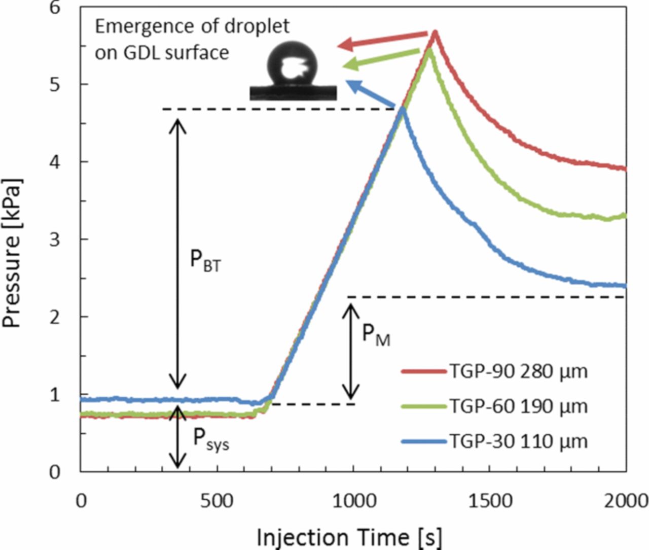
Figure 16. Breakthrough pressures as a function of injection time (left) and as a function of PTFE loading in the GDL (right) (figure reprinted from Ref. 259 with the kind permission of the publisher).
In terms of in-situ testing, it has been shown that pressure forces can impact the water-removal rate by removing the droplets.251,256 High-resolution images have also been used to elucidate the dynamic behavior of liquid water on a GDL surface, including droplet coalescence, detachment by the gas core flow, and wicking onto hydrophilic channel walls (see Figure 14).251,256,257 For example, droplet detachment as a function of gas velocity is shown in Figure 17.257 Real-time images of water transport through the GDL were also captured by Litster et al. using fluorescence microscopy, which allowed for pore-level detail.260 They observed the dynamic behavior of water traveling through specific pathways of the GDL and concluded that capillary fingering was the primary mechanism by which water traverses the pore network.
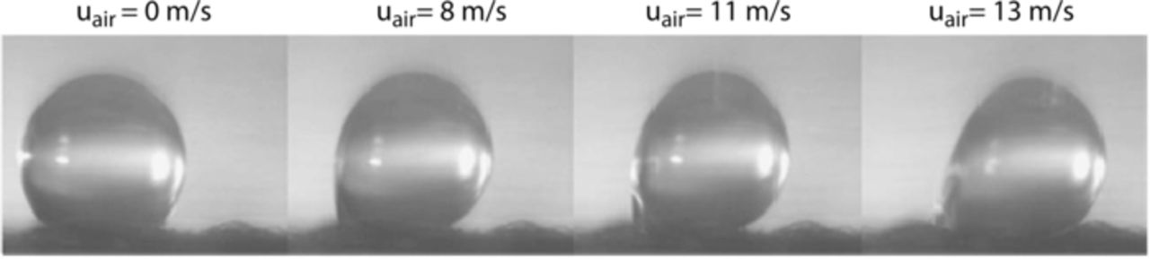
Figure 17. Sequence of surface distortion of a 1.0 mm droplet before detachment from GDL surface.257
To understand the process of detachment, a force-balance approach can be used,
![Equation ([99])](https://content.cld.iop.org/journals/1945-7111/161/12/F1254/revision1/jes_161_12_F1254eqn99.jpg)
where Fa is the adhesion or surface-tension force, Fp is the pressure force, Fs is the shear force acting on the droplet, and Fg is the gravitational force, which is negligible for typical droplet sizes although can be more important for larger slugs. The pressure and shear forces are readily calculated from correlations and flow equations through the channel and associated drag effects.253,254,261,262 For example, the shear force can be calculated based on Stokes flow past a sphere and the shape of the droplet,
![Equation ([100])](https://content.cld.iop.org/journals/1945-7111/161/12/F1254/revision1/jes_161_12_F1254eqn100.jpg)
where d is the droplet diameter at its maximum, H is the channel height, ⟨v⟩ is the average flow velocity in the channel under laminar flow,83 μ is the fluid viscosity, and h is the droplet height.
However, the adhesion force, which represents the resistance force that a droplet needs to overcome to initiate motion along a surface, is not as straightforward. Typically, this has been correlated to the static contact angle and contact-angle hysteresis. However, since the GDL surfaces are rough, it does not provide an accurate estimation of the adhesion force between the liquid-water droplet and GDL surface. In addition, measurements based on the static contact and contact-angle hysteresis seem to be more qualitative than rigorously quantitative in terms of droplet mobility. A recent study shows that the sliding-angle experiment provides a better measure of droplet mobility and detachment from a rough and porous surface, like GDLs.156 The sliding-angle experiment measures directly the sliding angles and adhesion forces for liquid-water droplets on GDL surfaces,
![Equation ([101])](https://content.cld.iop.org/journals/1945-7111/161/12/F1254/revision1/jes_161_12_F1254eqn101.jpg)
where ρ is the water density, V is the droplet volume, g is the gravitational acceleration constant, θs is the sliding angle, and dw is the wetted diameter, which is the diameter of the contact area between the liquid-water droplet and GDL surface. Experiments have also shown that a bottom injection, as in a PEFC, demonstrates a much larger adhesion force due to the underlying liquid network than a top placement, which many studies use.156,259
As seen above, the key issues for the GDL / flowfield interface are in understanding the water removal into the channel. As discussed, multiple mechanisms including capillary interactions on the channel walls, condensation due to PCI flow, and droplet removal due to force balances can all contribute to the water removal. In addition, changes in liquid pressure due to droplet emergence and breakoff impacts the overall liquid holdup in the cell. Seeing as these effects are stochastic and complex in nature, delineation of the correct interface conditions for models has yet to be obtained and validated.
Catalyst-Layer Modeling
In catalyst layers, all of the species and phases discussed above exist in addition to source terms for heat, reactant consumption, product generation, etc. Thus, the conservation and transport equations delineated in above sections are used for modeling, as well as the multiphase flow treatments discussed above. Figure 18 shows a schematic representation of oxygen transport into and through the cathode catalyst layer. Here, one can see that multiple transport mechanisms occur. Due to the pore size, transport through the catalyst-layer thickness is dominated by Knudsen diffusion (equations 16 and 18). At the local length scale, transport through an ionomer and/or water films can become limiting, especially for low catalyst loadings. In terms of the agglomerate, while it is known that primary particles agglomerate during formation, the resultant secondary particles are not necessarily believed to be large enough to have significant transport resistances. In this fashion, agglomerates may not exist and then the agglomerate model results in a standard porous electrode one. In many ways, the agglomerate model approach provides an additional parameter to modulate the transfer current density, and although maybe not entirely physical, it does allow insight and better model predictions; it is the standard approach taken for continuum modeling. Furthermore, both the anode and cathode catalyst layers should be modeled in the same fashion, where the anode will have a sharper reaction distribution due to the faster HOR kinetics and lower hydrogen transport limitations.
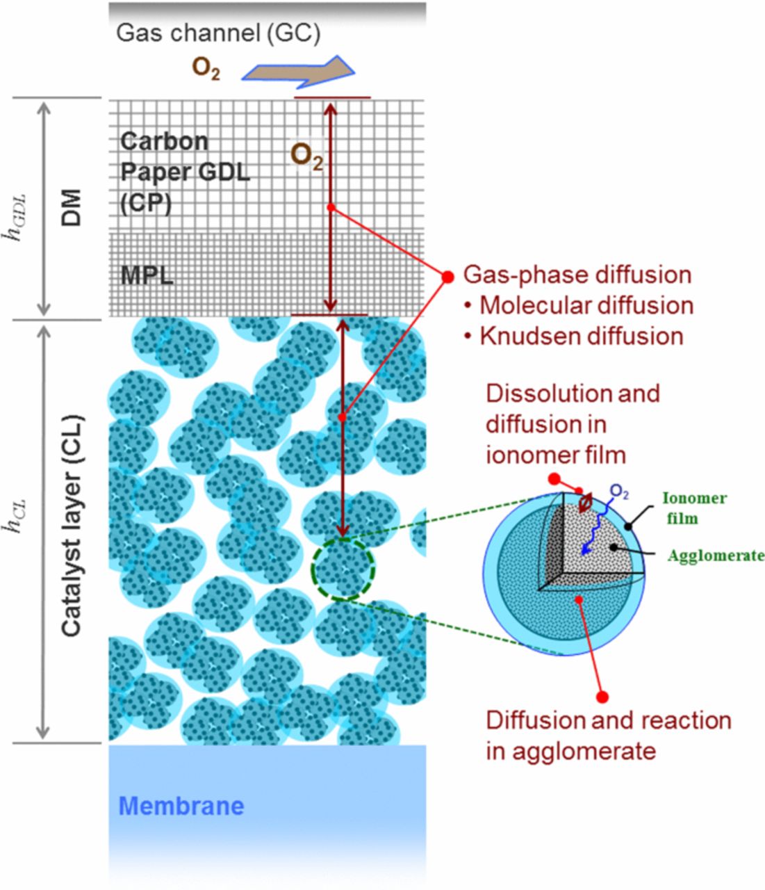
Figure 18. Schematic of oxygen transport phenomena into and through the cathode catalyst layer (image courtesy of Nobuaki Nonoyama).
Depending on catalyst-layer structure, two different modeling approaches have been employed that focus on low catalyst loadings: homogeneous model134,263–265 and agglomerate model,132,133,266,267 both of which adapt the previous modeling methodologies (described in more detail below) to this situation. Most homogeneous models apply to an electrode with homogeneous properties and structure in which primary Pt/C catalyst particles are coated with an ionomer thin-film and the effectiveness of electrochemically active Pt surface is 100%. This is typically not the case for standard catalyst layers. A notable exception is the model of Debe265 that used the kinetic theory of gases to derive the probability of oxygen reaching a greatly dispersed Pt site to explain the observed increased resistance at low Pt loadings.
The best approach for modeling a catalyst layer would be direct simulations through the actual structure. The reason is that the structures themselves are very heterogeneous and complex, and thus a macrohomogeneous approach may not capture many of the phenomena and interactions occurring. Similarly, unlike the DM, the microstructure complexity demands more complex models than a pore-network-model approach. However, due to the extremely small pore sizes and the same very complex structures, both virtual reconstructions (as described in a section above) and actual images are not readily available, with only a few studies on the structures.268–270 In fact, there is still debate as to how the ionomer is distributed in the cell as well as particle sizes, etc.271–274 For example, although often over-looked, it is believed and been shown through some computations that Nafion ionomer does not penetrate the smaller (primary) pores (O(20 nm)) that may exist within the agglomerates in PEFC catalyst layers.275–282 This is quite reasonable since the primary structures of Nafion are 30 nm long single chains of ionomer with a diameter of 3 to 5 nm,283 or larger aggregates.284,285 Therefore, even though Nafion is known to adsorb on carbon-black surfaces,269 as also discussed for thin-films below, the Nafion aggregates cannot easily enter the smaller primary pores of Pt/C agglomerates. Thus, the internal areas for reaction may indeed by filled with water or perhaps only by vapor. On top of these complexities is the fact that the structure is not stagnant and evolves during cell operation. For these reasons, macroscopic approaches are still used. Characterization of the catalyst-layer structure and related variables under operating conditions remains a critical need for future model development and validation.
In the subsections below, we examine the critical issues of catalyst-layer modeling across multiple length scales, but with an emphasis on the continuum approaches. First, the treatment of macroscopic modeling of transport in the catalyst layer is presented. Next, the issues that arise with ionomer thin-films within the catalyst layer are discussed, followed by examining mesoscale modeling of transport that necessitates the use of double-layer phenomena. Finally, catalyst-layer degradation and its association with transport modeling is discussed.
Microscale simulations and reconstruction
Similar to the reconstruction and microscale simulations of DM described in the multiphase flow section, one can also do similar analysis for the catalyst layer.286–295 However, since it is a much more complicated structure with much smaller domain sizes and a lower amount of knowledge and imaging, such simulations and stochastic reconstructions are challenging, with limited image-based approaches being used.294 The challenge is offset by the need since catalyst layers are the most important layers. As discussed in the section related to DM, the numerical techniques used for analysis tend to be independent of the method used for reconstruction. Monte Carlo, finite element, finite volume, and lattice-Boltzmann techniques have been commonly applied, but there is still a need for greater understanding of the interaction between materials, particularly the interfacial behavior. For example, as discussed below, ionomer thin-films seemingly are important, but their incorporation and modeling in microscale models is in its infancy. At this stage it is not clear if this type of behavior requires a different set of physics in order to describe it or if the current numerical methods imposed to undertake analysis on the digital reconstructions are sufficient to accommodate those changes.
Early reconstructions focused on large particles287 or lattice techniques.249,251,254,255 One of the key questions between the two approaches is whether the resolution of the particles and overall domain is sufficient to determine accurate estimates of the transport properties for the medium. The lattice-based approaches typically have relative domain sizes that are larger as different control volumes can be simply specified to belong to a specific phase (ionomer, carbon, platinum, or pore), where as in the particle approach there will exist many control volumes within a particle such that transport within the particle or across the interface are well resolved. It would seem reasonable to assert that the success or failure of either of the two approaches will be a large function of whether the size of the total domain or the interfacial-area aspects dominates the transport phenomena of interest.
More recent efforts try to closer recreate the actual manufacturing process. For example, it is possible to apply rule-sets (similar to that done for the GDL), where one can start with a carbon particle distribution based on the criteria of constrained overlap as shown in Figure 19a. After the placement of the carbon, the platinum is deposited by randomly seeding a location on the carbon surface similar to a functionalized site that would be available in the real process for platinum deposition. This functionalized surface is then subjected to simulated particle deposition and growth that is intended to simulate platinum plating, shown in Figure 19b. Finally the resulting carbon/platinum structure is intruded with an ionomeric phase resulting in the digitally reconstructed morphology, Figure 19c. This intrusion is based on placing ionomer via a stochastic algorithm on carbon either as deformable particles or chain by chain based on its base chain length. In either case, if the pores are too small compared to the particles or the chain, then the ionomer cannot enter into the pore space. Simulations can then be carried out on these microstructures to determined effective properties.
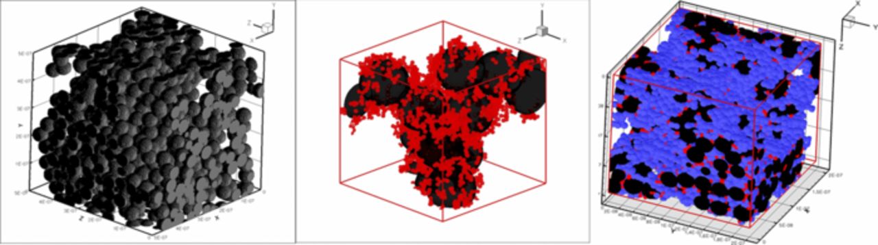
Figure 19. Chaining-rule-set stochastic simulations to reconstruct catalyst layers starting with (a) carbon particles, the (b) seeding/plating deposition of Pt, and finally (c) ionomer intrusion based on a sticking probability algorithm.
The aspects of the reconstruction methods underlies a specific reality related to the catalyst layer, which is that to-date key behaviors related to how the microstructures are formed are not fully understood. The development of catalyst-layer formation models are a key area for on-going research with only a few selected publications in the area.268 Other representation on the molecular-dynamics scale have been attempted to further provide characterization of the individual constituents that make-up the layer itself.296,297 In particular though, questions about the phase-segregation that occurs with ionomeric materials, the associated processing methods, additives, and surface-interactions between the materials within ink solutions are of interest. It is also interesting to consider that this aspect of manufacturing and the associated uncertainty around the physics of formation that lead to one of the primary differences in considering the current methods of stochastic and image-based reconstruction, in that the stochastic reconstructions are meant to encompass the range of variability seen from this formation process.
Transport within catalyst layers
The key for modeling catalyst layers is developing the correct expressions for the transfer current between the electron- and proton-conducting phases that represents the reaction as a function of local conditions. As noted, the methodologies for effective properties and multiphase and energy transport across the layer are handled in the same manner as with the DM, albeit with more complicated expressions due to the more complex and heterogeneous structures. For the ionomer thin-films in the catalyst layer, the same approaches as for the bulk membrane can be used (see equations 37 and 38). However, recent studies on the underlying knowledge of the structure/function relationships of ionomer thin-films in the catalyst layers are beginning to show that such an assumption is poor as discussed in more detail below.157,298–305
The kinetic expressions, equations 58 and 60 for the HOR and ORR, respectively, result in a transfer current between the electronic-conducting (1) and ionic-conducting (2) phases (see equation 10), which is related to the current density in the two phases through equation 23 (neglecting double-layer charging)
![Equation ([102])](https://content.cld.iop.org/journals/1945-7111/161/12/F1254/revision1/jes_161_12_F1254eqn102.jpg)
Assuming the ORR is the only reaction that is occurring in the cathode (i.e., crossover and degradation reactions are ignored), the conservation equation 10 for oxygen in the cathode can be is written as
![Equation ([103])](https://content.cld.iop.org/journals/1945-7111/161/12/F1254/revision1/jes_161_12_F1254eqn103.jpg)
The interfacial area of the catalyst with respect to electrolyte and gaseous reactants, a1,2, is often determined by
![Equation ([104])](https://content.cld.iop.org/journals/1945-7111/161/12/F1254/revision1/jes_161_12_F1254eqn104.jpg)
where L is the thickness of the catalyst layer and mPt and Apt are the catalyst loading and specific surface area (which is typically derived from experiment). If there is liquid water in the catalyst layer, this is expected to block the reaction sites. To account for this, one can use an approximation to scale the reaction area306–310
![Equation ([105])](https://content.cld.iop.org/journals/1945-7111/161/12/F1254/revision1/jes_161_12_F1254eqn105.jpg)
where ao1, 2 is the specific interfacial area with no water blockage, and the saturation can be determined based on the methodologies described in the multiphase flow section. While simple, this approach is not rigorous nor really valid since oxygen can still be transported through water. Thus, a better approach is to use a film of water that is generated and retards the gas transport gradually. To do this, one can use the treatment described for thin-films in the next subsection,311,312 although the water thickness will vary with operating conditions, especially due to the local heating at the catalyst site. Modeling, clarifying, and describing these complexities is currently a research need.
The catalyst-layer pore structure can be classified into intra agglomerate and inter agglomerate pores where the agglomerate is essentially the mesoscale structures that contain the reaction sites (see Figure 18). The intra-agglomerate pores determine the utilization of Pt catalyst and inter agglomerate pores facilitate the transport of gases and liquid. The distribution of these pores determines the balance between the electrochemical activity with mass-transport phenomena. Describing the structure is one of the most complex efforts to be undertaken in transport modeling and is a key future area of integration for different models and modeling scales. Even in the continuum, macroscopic models there are essentially two major length scales that are considered depending on the inter- and intra-particle/agglomerate interactions. The former or layer length scale is treated using the approaches described in the preceding sections of this review, although with the porosity given by
![Equation ([106])](https://content.cld.iop.org/journals/1945-7111/161/12/F1254/revision1/jes_161_12_F1254eqn106.jpg)
where Ri/j stands for the mass ration between species i and j and the subscripts C and I denote carbon and ionomer, respectively. The ionomer volume fraction is written as
![Equation ([107])](https://content.cld.iop.org/journals/1945-7111/161/12/F1254/revision1/jes_161_12_F1254eqn107.jpg)
These volume fractions are used for the macroscopic transport equations for the gas and liquid phases, where a Bruggeman type expression is used unless there is more detailed knowledge such as mesoscale simulations to determine the properties.277,313
As noted, to model the catalyst layer does not require new equations per se. However, for macroscopic simulations, one would like to use the microscopic phenomena but applied at the macroscopic scale. Such an effort can be achieved by using scaling expressions determined through mesoscale and other modeling approaches, or by modifying the transfer-current source term to account for diffusional losses at the agglomerate or reaction scale. The agglomerate model considers simultaneous reaction and diffusion into an agglomerate where there are numerous primary Pt/C catalyst particles homogeneously mixed with ionomer (see Figure 18).1,21,281,314–322 As mentioned, this assumption idealizes the local structure, but does allow for better model predictions; discussions on the impact of the local effects are made in the next sections. Within the agglomerate, isothermal and isopotential conditions are conveniently assumed. The validity of such assumptions were examined based on the magnitude of thermal and ionic transport properties.133 The impact of different kinetic and boundary conditions was also recently analysed along with the above assumptions with a full 2D(1D) model, showing that even when the ionomer conductivity is 1 × 10⁻⁴, the effects on cell performance are insignificant due to reaction re-distribution within the electrode.124
The diffusion and reaction into a spherical agglomerate is given by the equation (see equation 10)
![Equation ([108])](https://content.cld.iop.org/journals/1945-7111/161/12/F1254/revision1/jes_161_12_F1254eqn108.jpg)
where the effective diffusion coefficient is through the agglomerate. To understand the impact of the agglomerate, an effectiveness factor can be used, which is defined as the ratio of the actual reaction rate to the rate if the entire interior surface is exposed to the conditions outside of the particle1,323
![Equation ([109])](https://content.cld.iop.org/journals/1945-7111/161/12/F1254/revision1/jes_161_12_F1254eqn109.jpg)
where Ragg is the agglomerate radius and  is the reaction rate of the ORR at the surface conditions,
![Equation ([110])](https://content.cld.iop.org/journals/1945-7111/161/12/F1254/revision1/jes_161_12_F1254eqn110.jpg)
Thus, one can write the transfer current as
![Equation ([111])](https://content.cld.iop.org/journals/1945-7111/161/12/F1254/revision1/jes_161_12_F1254eqn111.jpg)
For a first-order reaction (m0 = 1), the simultaneous diffusion and reaction into a spherical agglomerate (equation 108) can be solved analytically to yield an effectiveness factor expression of
![Equation ([112])](https://content.cld.iop.org/journals/1945-7111/161/12/F1254/revision1/jes_161_12_F1254eqn112.jpg)
where ϕ is the dimensionless Thiele modulus
![Equation ([113])](https://content.cld.iop.org/journals/1945-7111/161/12/F1254/revision1/jes_161_12_F1254eqn113.jpg)
which is a measure of the reaction rate to the diffusion rate. Similar expressions hold for other with minimal error.133,323
As noted in Figure 18, there are possible transport limitations external to the agglomerate due to water or ionomer films. This issue is a critical one moving forward and is discussed in more detail in the next section in terms of its existence, impact, modeling methodology, and underlying genesis.
Ionomer thin-films
The oxygen-transport resistance in a cathode has been measured by limiting-current measurements using diluted oxygen.266,324 It was found that the resistance increased as Pt loading decreased.132–134,264,266,325 The voltage-losses were found to scale with the Pt surface-area specific current density (as opposed to geometric-area specific current density) after correction for bulk (channels, DM, catalyst-layer length scale) transport losses by suitable models.263 The local resistance is thus assumed to exist at or near the Pt surface to account for the unexplained higher voltage loss associated with lower Pt loading. As shown in Figure 18, the reactive sites (whether bare or in an agglomerate) are expected to be at least partially covered by thin-films of ionomer in order to provide proton conduction to the active site. In this confined structure, the properties are expected to differ significantly from the corresponding bulk membranes, meaning that one cannot treat the ionomer film in the catalyst layer as the same polymer used as the PEM.
It is known that the properties related to the transport functionalities of the ionomer in a catalyst layers differ from that of the bulk electrolyte. As shown in Figure 20, water-uptake isotherms for Nafion in the catalyst layers show much lower water contents compared to bulk Nafion membrane.157 Also, water uptake in catalyst layers has been shown to increase with increasing loading of platinum, which improves wetting properties and hydrophilicity,157,326 and with increasing ionomer content,326,327 although in general the catalyst layer's ionomer water uptake has been consistently shown to be depressed.157,327 With the lower water contents (and perhaps the existence of different morphology and confinement driving the lower water uptake), it is not surprising that the ion conductivity is likewise depressed,327–329 and is a function of ionomer content.326,327,330,331 However, it should be noted that some studies suggest similar proton conductivity in catalyst layers as in bulk,332,333 which may be due to measurement methods or perhaps anisotropic conductivity; more data is required. Finally, it is important to realize that understanding ionomer thin-film behavior is key not only for PEFC catalyst layers, but also for the characterization of bulk membrane surfaces, where the near-interface regions could be interpreted as thin-films.
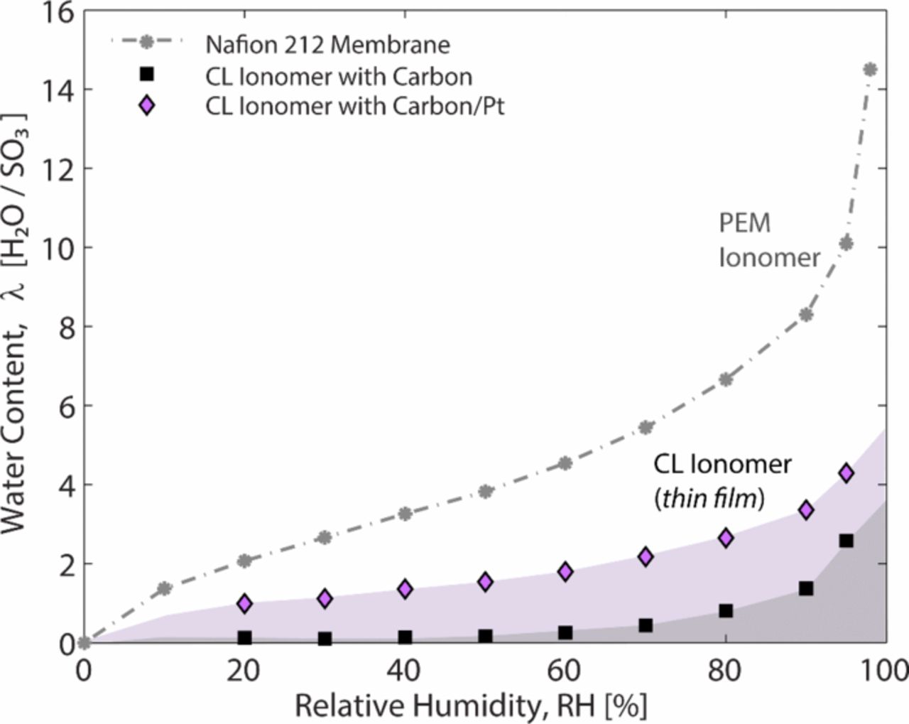
Figure 20. Water-uptake isotherms for Nafion in various PEFC catalyst layers as a function of relative humidity compared with that of bulk Nafion membrane.157
Ionomer thin-film modeling
As discussed above, the processes to model in the cathode catalyst layer include proton conduction and oxygen transport to the Pt surface where they react together with electrons to form water, which has to be removed from the electrode. In this section, we specifically examine modeling transport through the ionomer thin-film and its associated effects. Furthermore, as modeling liquid-water transport involves much complexity with a large amount of uncertainty (more data is required), the discussion below neglects liquid water. As the proton-transport resistance is needed to model proton conduction through the ionomer thin-film, this can be possibly determined from measured electrochemical impedance spectroscopy as a function of relative humidity and temperature,334,335 or derived from property relationships and is not discussed below.
When adding the film, the governing equation for oxygen transport (see equation 108) is altered to account for transport through the film and then reaction and diffusion into the agglomerate.159,311,312,336,337 For accounting for transport into and through the film, a two-stage process is used, comprised of transport through the film
![Equation ([114])](https://content.cld.iop.org/journals/1945-7111/161/12/F1254/revision1/jes_161_12_F1254eqn114.jpg)
and the slow oxygen dissolution process at the gas/ionomer interface,266,338,339
![Equation ([115])](https://content.cld.iop.org/journals/1945-7111/161/12/F1254/revision1/jes_161_12_F1254eqn115.jpg)
where afilm is the specific surface-area of the film,  is the rate constant for oxygen dissolution, H is Henry's constant, and
  is the equivalent pressure within the ionomer at the interface with the gas. Combining the above expression with that of equation 114 and assuming a linear gradient in the very thin film, results in
![Equation ([116])](https://content.cld.iop.org/journals/1945-7111/161/12/F1254/revision1/jes_161_12_F1254eqn116.jpg)
where  is the transport resistance of oxygen through ionomer film,
![Equation ([117])](https://content.cld.iop.org/journals/1945-7111/161/12/F1254/revision1/jes_161_12_F1254eqn117.jpg)
Alternatively, if one does not independently know the solubility and diffusivity, then the permeation coefficient ( ) can be used. In addition, since the film thickness and its transport properties are typically both unknown, one can just use the resistance for modeling.
At steady-state, the flux given by equation 116 is equal to the flux due to reaction and diffusion in the agglomerate; therefore, the unknown concentrations can be replaced. Using the resultant expression in the conservation equation 23 yields
![Equation ([118])](https://content.cld.iop.org/journals/1945-7111/161/12/F1254/revision1/jes_161_12_F1254eqn118.jpg)
and a similar one can be derived for the HOR.1,142
The above expression is the governing equation for the transfer current density and includes both the film and agglomerate resistances. Upon inspection, one can see that as the current density increases (i.e.,  increases), the film resistance becomes more significant and limiting. Thus, the impact of the ionomer thin-film on cell performance is expected to be more pronounced at low Pt loading due to the higher local oxygen flux to each reaction site.
As mentioned, the local resistances to the Pt surface increase with decreasing Pt loading. For example, Nonoyama et al. measured the local transport resistances of ∼0.04 s/cm at 0.20 mg/cm2 and 0.06 s/cm at 0.10 mg/cm2, where the other transport resistances have been removed through systematic variations in gas composition and pressure.266 This increase could be due to decreased ionomer surface area for effective oxygen permeation and subsequent higher fluxes through the ionomer thin-film to reach the catalyst site.133,266 Alternatively, ex-situ measurements have been made to determine the local resistance. The diffusion-limited current density in a planar Pt electrode with spin-coated ionomer thin-films was measured as a function of film thickness, and the local resistance was obtained by extrapolating the reciprocal limiting current density to zero film thickness.338,339 With the assumption that the resistances result from slow oxygen dissolution from the gas phase into the ionomer, the local resistance was incorporated into the agglomerate model with the agglomerate size being a fitting parameter to match the measured cell performance. The resulting agglomerate size is close to the primary Pt/C catalyst particle size, consistent with microscopy observation of the catalyst layer, which did not reveal any large agglomerates.338
The local resistance has been measured in-situ and ex-situ for use in predicting the performance of the low Pt-loaded electrodes. However, its origin is still unclear. Hypothetically, the local resistance can be attributed to slow oxygen dissolution process at the gas/ionomer interface,266,338 and/or strong interaction between the Pt surface and the sulfonate groups in ionomer leading to either a decrease in the effective Pt surface area, or ionomer structural changes in the thin-films near the Pt surface that lowers oxygen permeability as discussed below.340 Thus, the measured local resistance is a sum of three components from gas phase to the Pt surface: the interfacial resistance at the gas/ionomer interface, the bulk resistance of the ionomer film, and the interfacial resistances at ionomer/Pt interfaces. Quantification of each resistance would provide fundamental knobs to mitigate the voltage losses due to the local resistance via a combined modeling and experimental approach.
The relative importance of the two interfacial resistances was investigated by modeling the performance and limiting-current measurements on cathodes having the same thickness, ionomer content, and macroscopic structure but different Pt loading.341 The Pt nanoparticle distribution was varied by diluting various wt-% Pt/C catalysts with bare carbon support. The experimental data show that at a given Pt loading, voltage loss increases with Pt particle density and the electrode resistance trends accordingly as shown in Figure 21. The model-data comparisons demonstrate that the two interfacial resistances are equally important, particularly for the low Pt-loaded electrodes made of high wt% Pt/C catalyst.341 As shown in Figure 21b, the incorporation of the interfacial resistance is key for matching the data. This analysis stresses the need for incorporating the distributed resistances at the thin film (e.g., equation 117) in more detailed models for performance prediction and electrode design for both the anode and cathode. However, recent modeling124 of a cathode agglomerate model including both a Henry's law boundary condition and the dissolution boundary condition (equation 117) embedded in a 2-D MEA model demonstrated that the dissolution boundary condition has a negligible impact on cell performance unless the dissolution rate is reduced by at least an order of magnitude compared to reported experimental values.338 For lower dissolution rates, a reduction in agglomerate effectiveness and a better reaction rate distribution was observed. Both models and especially novel experiments are critical areas for quantifying and understanding thin-films and their impacts on PEFC performance.
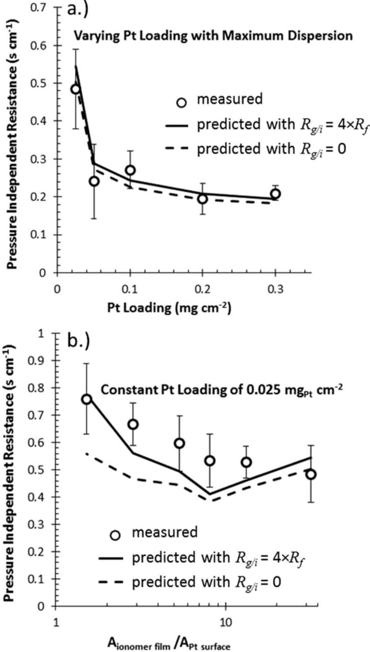
Figure 21. Pressure-independent oxygen transport resistance from single-particle model and experiments as a function of ionomer film to Pt surface area ration for (a) varying Pt loading with most dispersed samples (no bare carbon dilution) and (b) constant Pt loading with varying Pt dispersions. Reproduced from Reference 341.
Ionomer thin-film structure
In the previous sections, we examined the possible importance of ionomer thin-films in impacting the reactant mass transport to the electrocatalyst site and the overall electrochemical response of the system. One expects that as the ionomer thickness decreases from a membrane to a thin-film, associated transport properties could exhibit strong deviations from their bulk-polymer values. For example, one can envision that the ionomer thin-film may behave entirely like the interface in a PEM.327 It is well known that the behavior and properties of the ionomer are controlled by a balance between the chemical (or solvation) and mechanical (or deformation) energies,63,93,94 and thus exploring the structure of ionomer films on various substrates is a worthwhile endeavor.
When a polymer is confined to thicknesses comparable to its characteristic domain size, its properties and morphology differ from the analogous bulk materials.342–346 Even though confinement effects in polymer films have long been of interest, films of phase-separated ionomers, such as perfluorinated-sulfonic-acid ones, have gained attention only recently due to their complexity and ill-defined structure.298–304,347–349 Most studies investigate Nafion thin-films on the commonly used silicon substrate, where decreases in water content or swelling,299,350,351 ionic conductivity,300,302,352 and/or mobility and diffusion,298,299,301 have been reported as shown in Figure 22. The exact magnitude of these changes largely depends on the processing conditions, thickness, and the substrate. In general, for Nafion thin-films, a significant deviation from bulk behavior is observed in uptake and related transport properties when the films are confined to thicknesses of less than 100 nm, with initial deviations occurring up to almost 1000 nm. Typically, there is a decrease in water content until one gets to very thin-films (<20 nm) where seemingly the lack of being able to form crystallites results in an increase of water content.300,305 The values and trends are in agreement with those derived from catalyst-layer studies (see Figure 20) in terms of both water contents as well as time constants for water uptake,157,300,327 thereby suggesting that ionomer thin-films can serve as model systems to examine transport phenomena in catalyst-layer ionomers. A lower conductivity and increase in activation energy was reported for thinner films which suggest intrinsic changes in morphology controlling the conduction mechanisms.302,352,353 The observed reduction in transport properties is consistent with the measured increase in modulus of the thin-films with decreasing thickness.354
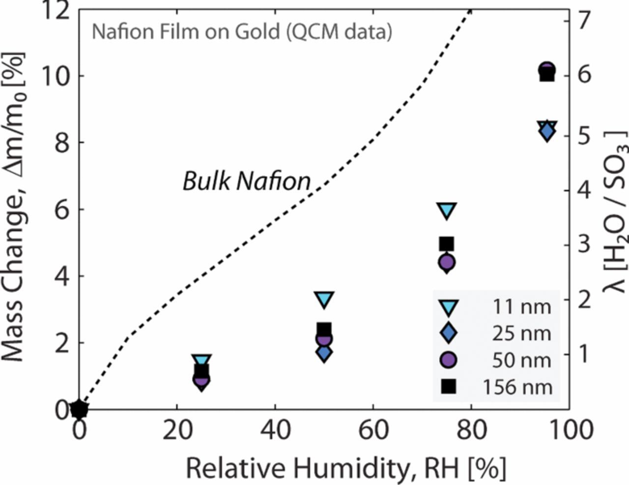
Understanding the origins of these confinement-driven changes in transport properties is possible only by exploring the surface structure and internal morphology of the thin-films. Recent studies have demonstrated that confinement effects and wetting interactions result in different surface and near-edge morphological properties of thin-films as shown by grazing-incidence small-angle X-ray Scattering (GISAXS),300,305,348,350,351 reflectivity,350,355 AFM,300,348,353,356,357 TEM,300 fluorescence,299 and positron annihilation.356 The results demonstrate a loss of phase separation as the thin-film thickness decreases as well as possible ordering depending on the substrate. Recent studies on metal and carbon substrates suggest that domain orientation closer to the support could be parallel to the substrate or random and perhaps exhibit specific adsorption and annealing behavior.305,355 Another evidence of change in the thin-film's surface morphology is the thickness-dependent surface wettability: thicker films have a hydrophobic surface whereas sub-50 nm thick films exhibit a hydrophilic surface,358 which is in agreement with simulation studies showing Nafion chains attach to graphite substrate surface.273 Such changes in wettability will have implications on the hydrophilicity/hydrophobicity of pores within the catalyst layer and associated transport phenomena. Thanks to the recent studies on Nafion thin-films reporting confinement-driven changes in properties, it has been acknowledged that the current understanding is still far from complete due to the significant material-parameter space for thin-films compared to the bulk (e.g., film thickness, casting and processing conditions, substrate, etc.).
Once understood, ionomer/substrate interactions at nanoscales can be exploited to model structure/property relationship of catalyst layers at mesoscales. For instance, using dissipative particle dynamics, conductivity in CL ionomer on a carbon support was shown to be anisotropic due to the layered structure in the electrolyte.359 Since orientation of water domains in thin films are already observed to change with wetting interactions and substrate (using GISAXS), advances in experimental and simulation techniques must be taken advantage of to obtain more information on size-distribution and orientation of domains. Only by understanding the role of film thickness and substrate/film interactions in structure/functionality of thin-film ionomers on PEFC relevant substrates and conditions, can one develop tools to achieve optimum ionomer content, better Pt utilization or reduced Pt loading, and ultimately improved catalyst-layer performance. For the latter, there is still a critical need to explore the transport properties of thin-films including, but not limited to, oxygen transport, ionic conductivity, diffusivity, thermal properties, and mechanical properties, both in the plane and thickness directions. In addition, the ionomer/substrate interface must be studied in more detail, both experimentally and computationally, to unveil the nature of chemical interactions between the carbon and Pt substrates and polymer backbone, side-chains and acid groups, as well as their influence on transport of specifies, especially in the presence of water and other solvents. Such studies will not only reveal how the thin-films may affect transport, but also perhaps the poisoning effect of the ionomer on the catalyst.360,361 Finally, it is also important to monitor carefully the timescales during any experimental study to investigate the dynamics response and equilibrium behavior of thin films.
Mesoscale electrode analysis and ionomer-free electrodes
In this section, we discuss the analysis of mesoscale transport in catalyst layers. The prior sections focused on reconstructed catalyst-layer structure, multiscale modeling, and upscaling to macroscale transport properties. Such approaches often assume idealized Nafion/Pt interfaces. Below, the nonideal features of the electrode structure and the associated transport resistances are discussed. In particular, the impact and modeling of incomplete ionomer coverage on Pt/C catalyst as well as the physics of proton transport on next-generation ionomer-free electrodes are introduced.
An important class of alternative electrode architectures is ultra-thin ionomer-free electrodes, exemplified by 3M's nanostructured thin-film (NSTF) electrodes.362–364 These promising electrodes have thicknesses from 0.2 to 1 μm and are ionomer-free polycrystalline Pt whiskers that are partially embedded in the membrane upon cell assembly. They have demonstrated good mass activity and durability, but have been shown to be sensitive to flooding and liquid water, especially at lower temperatures, due to their thinness.364 It is desirable to pursue such structures, but questions remain regarding possible proton limitations and the ion-conduction mechanism.
Although experimental work on ion transport in ionomer-free regions is sparse, theoretical modeling of ion transport in these ionomer-free regions is even less developed. In state-of-the-art PEFC electrode models, it is often assumed that the primary pore structure is filled with Nafion281 or water365 and that the ionic transport within primary agglomerates is infinitely fast and any ohmic losses from within the agglomerate's primary pores are neglected.275–282 Yoon and Weber133 have shown that this is a reasonable assumption if the proton conductivity within the agglomerate is >0.001 S/cm. A conductivity in this range is consistent with a high volume fraction of Nafion and bulk-like Nafion conductivity. However, the effect of inter-agglomerate resistances could be significant in ionomer-free pores and in dry conditions.
Ion transport in ionomer-free zones
Nafion in PEFC electrodes acts as a proton conductor and its fixed high proton concentrations ensure that the ORR is not ion-transport limited. In ionomer-free zones of conventional PEFC electrodes and NSTF electrodes there is no Nafion to aid in proton transport. Ion conductivity of bulk neutral water is about seven orders of magnitude lower than that of Nafion. The question remains open regarding possible proton transport mechanisms present in the water-filled regions of PEFC electrodes. Over the past two decades two major transport mechanisms have been proposed to explain ion transport in ionomer-free regions: 1) adsorbed H-adatom diffusion along the electrode surface,366–369 and 2) water-mediated conduction of protons.370,371
Several studies have reported or investigated the electrochemical activity of ionomer-free electrode regions beyond the interface with the PEM.366–368,372,373 Beginning with the work of McBreen,366 the majority of studies have focused on evaluating ECSA with underpotential deposited (UPD) hydrogen in cyclic-voltammetry experiments.366–369 These experiments demonstrated that the entirety of the continuous Pt surface connected to the PEM was accessible to UPD hydrogen. However, it is apparent from those results (particularly from the work of Paulus et al. using model electrodes)367 that the electrode area is accessible because of faradaic reactions at the PEM interface followed by surface diffusion of the adsorbed hydrogen ad-atoms along the Pt/water interface (second proposed mechanism). Thus, although the Pt surface area is accessible by CV measurement, it is not necessarily electrochemically active. In terms of RH, several groups have reported up to a 50% drop in ECSA when the RH is reduced.374,375 Electrochemical-impedance-spectroscopy measurements have demonstrated that the conductivity of the water in electrodes without ionomer is many orders of magnitude higher than that of bulk water and approaches that of the Nafion in Nafion-bound electrodes.372,373,376
Recently, Litster and coworkers332,377 have performed directed measurements of electrode conductivity during PEFC operation using microstructured electrode scaffold (MES) diagnostics. They observed conductivities that were 3 to 4 times higher than expected from the bulk conductivity of Nafion and its estimate volume fraction and tortuosity in the electrode. This finding agrees with prior transmission-line analysis of N2/H2 impedance measurements,378 but contradicts ex-situ measurements observing reduced conductivity of Nafion thin-films as discussed in the previous section, but these films may be anisotropic.300,302 It was suggested that the increased conductivity was a result of surface-supported transport on the high-surface-area catalyst and proton transport through water films (second proposed mechanism). Again, there was a strong dependent on RH with significantly lower conductivity at RH < 60%. Finally, one should also note that during operation, there are often either contaminant ions or membrane-degradation products, which can alter the charge-carrier concentration and ionic strength of the water.
There are only a few modeling studies addressing proton transport in Nafion-free electrode domains.371,379–381 The Poisson-Nernst-Planck equations (28 and 24) can still be applied to describe ionic concentrations and potential distributions within water-filled domains. These continuous equations do not accurately describe the physics in the vicinity of the water/electrode interface because they assume ions to be point charges and the solution to have a constant dielectric permittivity. Under high applied electric fields or when ion concentration in solution is high, the Poisson-Nernst-Planck theory does not handle well the ion crowding effect at the interface. Essentially, it states that the electrode can be charged to an infinite capacity. There is also a finite physical limit to how closely solvated ions can approach the electrode. When electric potential is applied to the electrode, there is a preferential orientation of solution dipoles induced by the electric polarization. In Poisson's equation (24), the dielectric permittivity has to be reduced to account for this interfacial polarization. Given these limitations to the applicability of the continuous Poisson-Nernst-Planck equations and constrained, mesoscale geometries of the electrode domains, there is a need of a model that can address these challenges. For decades, EDL theories have been effectively complementing Poisson-Nernst-Planck theory, bridging these continuum equations with discrete physics at the solution/electrode interfaces.
Electric-double-layer model for a PEFC electrode
Whenever there is an interface separating solid and liquid, the mobile species such as ions, electrons, and water dipoles will orient in a way to minimize the free energy of these two phases.89 In general, EDLs form at solution interfaces due to surface dissociation/association reactions, specific adsorption, applied potentials, and ionomer layers. Figure 23 shows the general EDL structure for a positively charged electrode (e.g., a PEFC cathode). The positive surface charge is due to a depletion of electrons caused by electrochemical polarization of the electrode. Next to the solid surface are three main double-layer regions: (1) the compact, Stern layer, (2) the diffuse layer, and (3) the bulk, electrically neutral solution. This conceptual model is termed the Gouy-Chapman-Stern-Grahame (GCSG) model. The GCSG model is the most comprehensive form among the EDL models showing good agreement with experimental capacitance measurements. In this microscopic model, a local electroneutrality exists between the charge in solution, qs, and that on the metal surface, qm,
![Equation ([119])](https://content.cld.iop.org/journals/1945-7111/161/12/F1254/revision1/jes_161_12_F1254eqn119.jpg)
where qd is the charge in diffuse layer, which arises from competing migration and diffusion processes, and qH is the charge within the Stern layer.382 The plane between the Stern and diffuse layers is termed the outer Helmholtz plane (OHP) – the plane of closest approach for fully-solvated ions. In this case, partially solvated ions are located within the Stern layer with their centers along the inner Helmholtz plane (IHP). Although hydrodynamically immobile, ions in the Stern layer are known to have mobilities on the same order as the bulk and can be a large contributor to the ionic conductivity in capillaries and porous media.
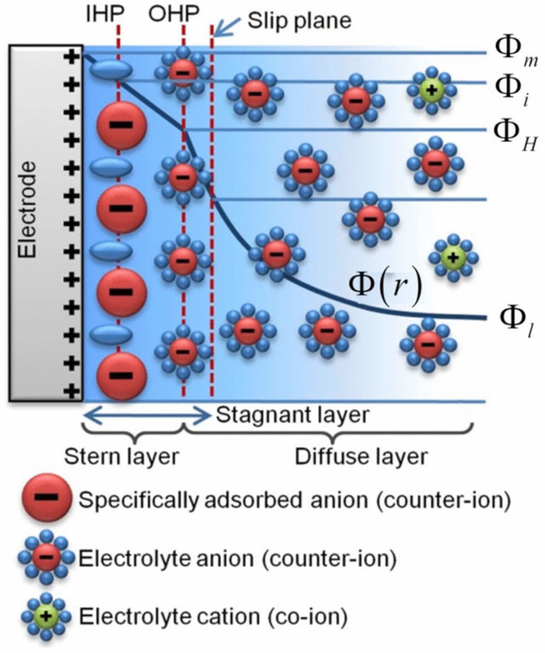
Figure 23 Schematic of an EDL according to the GCSG model for a positively charged electrode with adsorbed anions at the IHP. The slip plane and the edge of the diffuse layer are considered not co-located in this schematic. Not to scale.
As Figure 23 shows the GCSG model implies that the potential difference between the electrode, Φm, and bulk liquid, Φl, has two contributions:
![Equation ([120])](https://content.cld.iop.org/journals/1945-7111/161/12/F1254/revision1/jes_161_12_F1254eqn120.jpg)
where ΦH − Φl is the potential drop within the diffuse layer and Φm − ΦH is that within the Stern layer. For interfaces with thin double layers (i.e., PEFC electrode|Nafion interface) most of the potential drop occurs in the Stern layer. For water-filled pores of PEFC electrodes with thick and overlapped EDLs (due to low ionic concentration and confined geometry) the potential drop within the diffuse layer contributes significantly.
Commonly, water-filled pores within porous PEFC electrodes and water films on NSTF electrodes are modeled with simplified cylindrical axisymmetric domains.371,380 Poisson-Nernst-Planck theory formulated by equations 24 and 28 describes transport of ions and potential distributions within the diffuse layer. For cylindrical pores, analytical solutions exist for equilibrium EDLs where Poisson-Nernst-Planck equations simplify to the Poisson equation with a Boltzmann distribution for ions (see equation 25).383–386 This formulation is restricted to ion transport in radial direction and assumes that the pore centerline potential is constant in the axial direction. The solution to the potential distribution within the diffuse layer is
![Equation ([121])](https://content.cld.iop.org/journals/1945-7111/161/12/F1254/revision1/jes_161_12_F1254eqn121.jpg)
where b depends on the electrode surface charge or applied potential, r is a radial distance from the center of the pore, and Φ(r) is a potential within the pore relative to the centerline pore potential. Water-filled pores are bounded on the outside by Nafion film with high proton concentration balanced by the sulfonic-acid groups. Within Nafion, the potential can be assumed to be Φ0 = 0 referenced to SHE as the electrochemical condition within the bulk Nafion phase approximates a low-molarity strong-acid electrolyte. Due to orders of magnitude difference in ionic concentrations for bulk water and ionomer, a Donnan potential difference describes the potential drop at the water|Nafion electrode. The Donnan potential difference effectively links the centerline water-pore potential and bulk Nafion. It can be approximated with the solution to Poisson-Boltzmann equation applied to a system with proton-penetrable membrane adjacent to water,387,388
![Equation ([122])](https://content.cld.iop.org/journals/1945-7111/161/12/F1254/revision1/jes_161_12_F1254eqn122.jpg)
where NN, H + is the density of charged groups within membrane and nH + is centerline concentration. To couple a diffuse-layer potential distribution described by equation 121 to the electrode potential or its surface charge, an additional boundary condition is required. A common approach is to separate interfacial differential capacitance into a series of capacitances.371,389–393 Dividing equation 120 by the metal charge and differentiating it, one obtains
![Equation ([123])](https://content.cld.iop.org/journals/1945-7111/161/12/F1254/revision1/jes_161_12_F1254eqn123.jpg)
![Equation ([124])](https://content.cld.iop.org/journals/1945-7111/161/12/F1254/revision1/jes_161_12_F1254eqn124.jpg)
where, C is the total interfacial capacity, CH is the Stern layer capacity, and Cd is the diffuse layer capacity. The next step is to apply Gauss's law to a control volume of the Stern layer, neglecting specific adsorption in the IHP and assuming metal to be an ideal conductor (electric displacement is zero). Along with integration of Stern-layer capacitance and setting a lower integration bound to the metal's potential of zero charge (PZC) a Robin boundary condition can be obtained,
![Equation ([125])](https://content.cld.iop.org/journals/1945-7111/161/12/F1254/revision1/jes_161_12_F1254eqn125.jpg)
where εr is a dielectric permittivity of Stern layer. Depending on the limits of integration, different variations of equation 125 exist in literature. The PZC is an important intrinsic physical property of the electrode that has often been overlooked in a modeling community. Herein, a brief discussion is provided.
When considering EDLs on metal electrodes, the amount of surface charge being balanced by the ions depends upon the difference between the electrode potential and its PZC, or more specifically, the potential of zero free charge. The PZC is the potential for which there is no free charge at the metal interface with the solution (i.e., there is no excess of positive or negative charge in the solution). Thus, if the ion concentration of the bulk is low (as in the case of pure water), the conductivity is extremely low at the PZC. For electrode potentials above the PZC, there is excess positive charge in the metal. Likewise, for electrode potentials below the PZC, there is excess negative charge in the metal. Considering the Pt-water electrode system, for potentials above the PZC, there is a depletion of protons, and, below the PZC, there are accumulated protons. For reference, experimental studies have determined the PZC of Pt to be between 0.2 and 0.3 V vs SHE (commonly taken to be 0.26 V vs. SHE)394,395
Overall, the capability of the EDL model applied to a PEFC water-filled electrode includes a prediction of local ion conductivity and radial, as well as axial, potential distributions within the pore approximated with a cylindrical geometry. The EDL model can be extended to include additional physics, such as: electrode's surface chemistry (e.g. surface-complexation model),380 electrode's electron spillover effect (e.g. space-charge layer),380,396 different solution impurities, and specific adsorption at the IHP (modified Stern isotherm). The EDL model assists with resolving mesoscale transport phenomena coupled to reaction kinetics. Under operating conditions in a PEFC, a current is drawn from the cell and the EDL model can predict local electrochemical reaction generation based on the local reactant concentrations and potential distributions. When the model incorporates both radial and axial dimensions, the reactant gas transport is modeled with Fick's law and the OHP is assumed to be a plane where the electrochemical reaction is occurring, as it is a plane of the closest approach for hydrated ions. Local current density is modeled with Butler-Volmer or Tafel equations with local OHP reactant and product activities. For macroscale transport models the reaction kinetics equations use the electrochemical reaction driving force between the bulk metal and electrolyte (or ionomer) phases. In the EDL models the local reaction overpotential, ηOHP, is the reaction driving force, which can be related to a macroscopic surface overpotential, η,
![Equation ([126])](https://content.cld.iop.org/journals/1945-7111/161/12/F1254/revision1/jes_161_12_F1254eqn126.jpg)
Essentially, the potential difference across the Stern layer is the reaction driving force in the EDL models. This potential difference adjustment is also termed the Frumkin correction.371,380,381,391,397–399 The diffuse-layer potential only affects the interfacial electrokinetics by modifying the activities of reactant species at the OHP.
Pore-level models
Macroscopic PEFC models that consider the presence of EDLs in water domains are few.371,379–381 As noted above, the electrode models utilize the Poisson-Nernst-Planck equations coupled with the above GCSG theory and a geometry often consisting of a water-filled pore with perhaps ionomer at one end. To couple the Poisson-Nernst-Planck equations with GCSG theory, the Poisson-Nernst-Planck steady-state equations (equations 28 and 24) are applied on ionomer and water domains. The aim is to solve for potential distribution and proton and hydroxide concentrations. These second-order differential equations require two boundary conditions for each variable. The electrode can be modeled as a 1D domain adjacent to the water. In the ionomer there are two types of ions present: negative sulfonic groups that are stationary, and mobile protons counterbalancing them. In the water domain, the transport of hydroxide and protons is modeled. The outer edge of ionomer serves as a reference for concentrations in the Nernst-Planck equation (e.g. setting them to bulk value in Nafion) and potential in Poisson's equation (0 V vs SHE). The second set of boundary conditions is considered along the water/electrode interface. For the Poisson equation, a Robin boundary condition (equation 125) should be applied, where Φm − PZC is the applied electric potential relative to the PZC (both are known), and  is constant (i.e., assuming Helmholtz capacitance is constant). For Nernst-Planck, insulation for hydroxide ions is used, whereas a flux of protons due to the reaction consumption (ORR in cathode) or generation (HOR) is specified. The reaction (e.g. ORR in the cathode) along the water/electrode interface can be described with Tafel equation (59), where the overpotential is set to equation 126 and local activities are used.
The simulation results of Chan and Eikerling371 provided two important pieces of insight into the effective operation of ionomer-free electrodes. First, they showed that the primary impact of ionomer-free zones is the reduced reaction current density due to the depletion of reactant protons, rather than a reduction in conductivity and a long-range transport limitation. Second, the work highlighted the critical importance of the metal electrode's PZC. In order for their model to achieve current densities consistent with those measured for the NSTF electrodes, they had to assume PZC values greater than 0.7 V; these values are well above the range of values experimentally measured for Pt electrodes.
Zenyuk and Litster380,381 calculated that incomplete ionomer coverage did not significantly influence a Pt/C anode's performance at PEFC current densities because protons are not a reactant for the HOR. More recently, the model was extended for Pt surface cathodes with ionomer, such as NSTF electrodes.381 The model included finite-thickness domains that captured the Stern layer and space-charge layer in the metal so specific adsorption and dipole contributions to the PZC could be included. In addition, due to large pH variations, the model included non-equilibrium water dissociation and hydroxide-ion transport, with the associated alkaline ORR mechanism. The results showed that the pH quickly increases away from the Nafion interface, particularly at high potentials near open circuit (much higher than the PZC). At a distance more than 10 nm away from the Nafion interface, the concentration of OH− is many orders of magnitude higher than that of H+. Thus, at high potentials, the ORR on Pt is dominated by the alkaline mechanism and the overall, high conductivity is due to the high concentration of OH−. This suggests the high conductivity measured experimentally may not be the conductivity of protons, but rather hydroxide ions. The results also show that as the potential is reduced, there is less proton exclusion from the pores and the acidic ORR mechanism provides a greater contribution to the overall current density.
While some progress and understanding has been made recently on mesoscale transport of ions and in ionomer-free electrodes, there is still much more work that is required going forward. For example, it is important to develop a modeling framework that can effectively scale-bridge the above single-pore and double-layer models with macroscopic PEFC models. In this fashion, issues such as water sensitivity simultaneous with proton sensitivity of ionomer-free electrodes can be studied, and optimized designs and operating schemes elucidated. There is also a need for further experimental studies into ionomer-free zones and electrodes in terms of identifying the EDL potentials, impact of surface structures, and ion mobilities. For example, ion mobilities at the interface, including within ice-like water structures400 and liquid/vapor-like interfaces401 are not well-resolved experimentally or by simulation. The proton mobility could be significantly increased within these water networks and could dramatically influence transport-model predictions.
Durability and degradation
The durability of PEFCs remains a major barrier to their commercialization for stationary and transportation power applications. Power transients, shut-down/start-up, temperature cycling, and RH cycling, are all operating conditions imposed by the rigid requirements of various applications. These operational transients induce a number of chemical and structural degradation mechanisms on MEAs that change the transport properties of both the materials and the structures, and consequently their performance.8,9 Major degradation mechanisms involve the catalyst layer and are reviewed below. These mechanisms include corrosion of the catalyst support, electrocatalyst degradation which includes platinum dissolution, migration and reprecipitation and loss of alloying constituents, and ionomer degradation and restructuring. These processes can cause changes in PEFC performance due to loss of catalyst utilization, electronic and protonic conductivity, and reduction in the transport rates of the gases and product water. Below, they are discussed in terms of their general impacts on transport modeling as well as modeling of the related transport processes themselves.
Carbon corrosion
A primary cause for changes in the structure of the catalyst layer is the corrosion of carbonaceous electrode supports leading to electrode collapse, changes in porosity, and reduced active catalyst area. The overall corrosion reaction of carbon in PEFCs can be expressed as402
![Equation ([127])](https://content.cld.iop.org/journals/1945-7111/161/12/F1254/revision1/jes_161_12_F1254eqn127.jpg)
Thus, this reaction is thermodynamically favorable at the potentials at which the cathode normally operates. However, the kinetics for carbon corrosion at normal cathode potentials is usually slow enough to support a decade of service life, although it should be noted that Pt greatly accelerates the rate of carbon corrosion.402 The reason for the slow kinetics has to deal with going through high-potential intermediates. Most mechanistic descriptions of carbon corrosion proceed through a carbon oxide or hydroxide intermediate. The following scheme is exemplary403
![Equation ([128])](https://content.cld.iop.org/journals/1945-7111/161/12/F1254/revision1/jes_161_12_F1254eqn128.jpg)
where C* is a carbon defect site. The C–OH group can be further oxidized to form a C=O group at a potential of E° = 0.8 V through the reaction
![Equation ([129])](https://content.cld.iop.org/journals/1945-7111/161/12/F1254/revision1/jes_161_12_F1254eqn129.jpg)
At a higher potential of E° = 0.95 V, the surface C–OH groups are oxidized to form carbon dioxide that exits the system leaving behind a new defect site,
![Equation ([130])](https://content.cld.iop.org/journals/1945-7111/161/12/F1254/revision1/jes_161_12_F1254eqn130.jpg)
This scheme captures the carbon dioxide emission at higher voltages from the oxidation of the unstable carbon surface.
As noted, kinetics typically are sluggish enough for carbon corrosion that in the typical PEFC potential range (0.0 to 1.0 V), there is not significant oxidation, especially below 0.9 V.404 A caveat is that carbon oxidation to CO2 can be measured and is promoted by potential cycling.405,406 The long-term relationship between carbon corrosion and load cycling (including open-circuit dwell time) is, as of yet, relatively undetermined. To incorporate and model carbon corrosion, a Tafel expression is used as the reaction is essentially irreversible,25,407
![Equation ([131])](https://content.cld.iop.org/journals/1945-7111/161/12/F1254/revision1/jes_161_12_F1254eqn131.jpg)
where the transfer coefficient is around 0.67, and the exchange-current density is on the order of 5 × 10− 18A/cm2 but with an activation energy of 134 kJ/mol.408 Thus, at high potentials and high temperatures the kinetics will become appreciable enough to drive the reaction. It is also known that the reaction rate is proportional to water partial pressure and logarithmic in time.404
From the kinetic expression and associated rate constants, one expects that at higher potentials, >1.2 V, carbon corrosion can proceed rapidly. Such high potentials have been shown to occur during start-up and shut-down or by local obstruction or starvation of hydrogen due to anode blockage or hydrogen depletion. This helps to explain why cells degrade more rapidly under cyclic conditions than they do when operated with fixed current densities and flows. Reiser et al. first explained the mechanism and presented a one-dimensional, steady-state model showing the development of large interfacial potentials in the hydrogen-starved regions.409 This reverse-current mechanism has been shown to exist, where potentials as high as 1.6 V have been measured when fuel and air coexist at the fuel electrode during start-up/shut-down events.410 The mechanism involves a current that is produced in the normal part of the cell driving that in the starved region as shown in Figure 24. In the hydrogen-starved region, the cell potential remains constant (shown by the dotted lines) but the local anode and cathode potentials vary due to a drop in the electrolyte potential such that the negative side undergoes ORR and the positive side undergoes carbon corrosion and oxygen evolution. Due to the high level of carbon corrosion from the high potentials created during H2/Air fronts and localized anode fuel starvation, these high potentials have been employed as accelerated stress tests for the catalyst support.
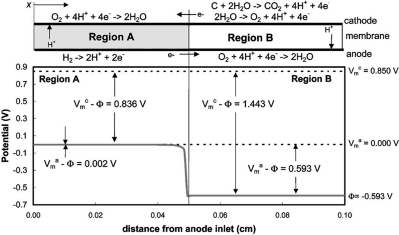
Figure 24. Potential distributions along anode flow path during reverse-current conditions (figure reprinted from Ref. 409 with the kind permission of the publisher).
To model such effects,404,408,411 one only needs the general transport equations described in the background section along with the carbon-oxidation-reaction rate equation 131 and with a Butler-Volmer equation 58 that includes oxygen evolution,
![Equation ([132])](https://content.cld.iop.org/journals/1945-7111/161/12/F1254/revision1/jes_161_12_F1254eqn132.jpg)
which occurs simultaneously with carbon corrosion at the higher potentials. To reduce the impact of the reverse-current mechanism, one can limit the gas transport through the membrane or short the stack,408 although in practice this is quite complicated because the hydrogen front does not reach each cell at the same time. Transient models that simulate the distribution of fuel from cell to cell during the introduction process are needed to optimize carbon-corrosion mitigation strategies.
Experimentally, carbon corrosion has been shown to have a number of effects on PEFC performance. These include changes to the electrocatalyst activity and kinetics, changing electrode-layer structure and porosity, and changing chemical surfaces which change the electrode-layer wetting properties (i.e., hydrophilicity); these combined effects are difficult to separate unambiguously and is an opportunity for modeling, especially these latter ones that directly impact the transport phenomena describe in this review. The associated effects of carbon corrosion on performance appear to depend upon many factors including the level and degree of carbon corrosion. As shown above, the carbon-corrosion process can be divided into two main reaction steps: (1) oxidation of the carbon surface to carbon-oxygen groups, and (2) further corrosion of the oxidized surface to carbon dioxide/monoxide.412 Carbon-surface oxidation increases the double-layer capacitance due to increased specific capacitance for carbon surfaces with carbon-oxygen groups.412 It may as well impact the wettability of the surface, making the carbon more hydrophilic and thus prone to flooding,413,414 which counteracts possible gains in porosity due to corrosion.415 Most studies, however, have demonstrated a loss in the cathode catalyst layer porosity,406,416,417 as shown in Figure 25, where approximately 50% of the porosity was lost within 10 hours of the accelerated stress test. Based on the electron microscopy observations of the centered-hollowed carbon particles and interconnected voids, it is concluded that carbon corrosion took place in an inside-out mode, with the carbon aggregate, rather than the carbon primary particle, as a basic corrosion unit.416 The size of carbon agglomerates decreased since carbon corrosion caused carbon particles to decrease in size. As carbon corrosion proceeds, the ionomer to carbon ratio of agglomerates increase,418 thus exacerbating possible mass-transport losses associated with ionomer films; to date still little is published on the overall interaction between the carbon surface and the ionomer in the catalyst layer under degradation. Overall, carbon corrosion results in a collapse of the electrode's porous structure and surface area,419,420 with loss of mass transport in the electrode, and subsequent degradation of PEFC performance.416 This effect is more severe underneath the flowfield lands, and especially on the anode land area where local fuel starvation may occur.421 A complete understanding of the cathode catalyst-layer water saturation, how that changes with durability and operating conditions and how catalyst-layer degradation changes is not yet adequate for a full development of being able to predict mass transport in these layers.
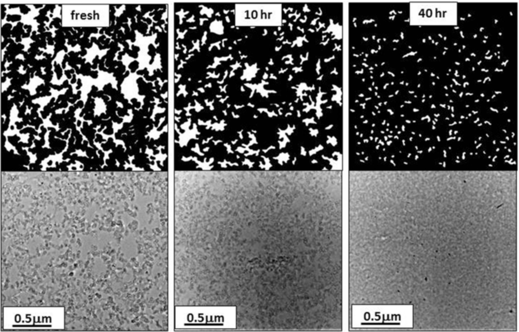
Figure 25 TEM micrographs of a cathode catalyst layer (a) fresh, and after a carbon corrosion accelerated-stress-test hold at 1.2 V (b) after 10 hr and (c) 40 hr.531
Finally, one should also mention the role of GDLs and MPLs on carbon corrosion, as they are integral for water management as discussed above. However, the exact effect that GDL/MPLs have on catalyst-layer carbon corrosion has been difficult to ascertain. Potential-hold testing for acetylene-black fabricated MPLs resulted in dramatic loss of cell performance, and the introduction of a graphitized carbon in the MPL reduced the current density loss by > 50%.422 Omitting the cathode MPL increased the rate of kinetic loss but slowed the mass-transport losses, also suggesting that the MPL itself was degrading during the accelerated stress test.423 In general, cells with MPLs appear to be more resistant to prolonged carbon corrosion.424 As discussed above, the interface between a Pt/C cathode and MPL has been shown to be distinct, where the MPL carbon retains its meso-graphitic structure and porous network (even adjacent to the cathode surface) whereas the carbon support used for Pt is fully oxidized.425
Platinum dissolution, migration, and redistribution
Studies show that Pt can dissolve in acidic media at pH values representative of the electrolytes in PEFCs,426–428 especially at higher potentials.429 As the potential is cycled from high to low, equilibrium moves Pt into solution, and back out of solution causing Pt redistribution.430 This is depicted in Figure 26a.431 Other mechanisms (depicted in the figure) which cause electrochemical active surface area loss include Pt particle migration (b), Pt particle detachment (c), and dissolution with precipitation in the ionomer phase (d). The effect of platinum redistribution leads to a loss in catalytic activity, reducing PEFC performance. The amount of Pt redistribution depends upon operating conditions including temperature, potential, RH, and presence of contaminants.432,433 Much of the loss of surface area is attributed to growth in platinum particle size in the catalyst layer. Coarsened platinum particles have been classified into two groups: spherical particles still in contact with the carbon support and nonspherical particles removed from the carbon support.434 The former results from electrochemical ripening, and the latter results from deposition in the ionomer by dissolved hydrogen. Both processes require preceding dissolution of the platinum. Pt dissolution/agglomeration can be diagnosed by a small decrease in limiting capacitance (the extent of which will depend upon wt-% Pt) and small change in electrode resistance.435
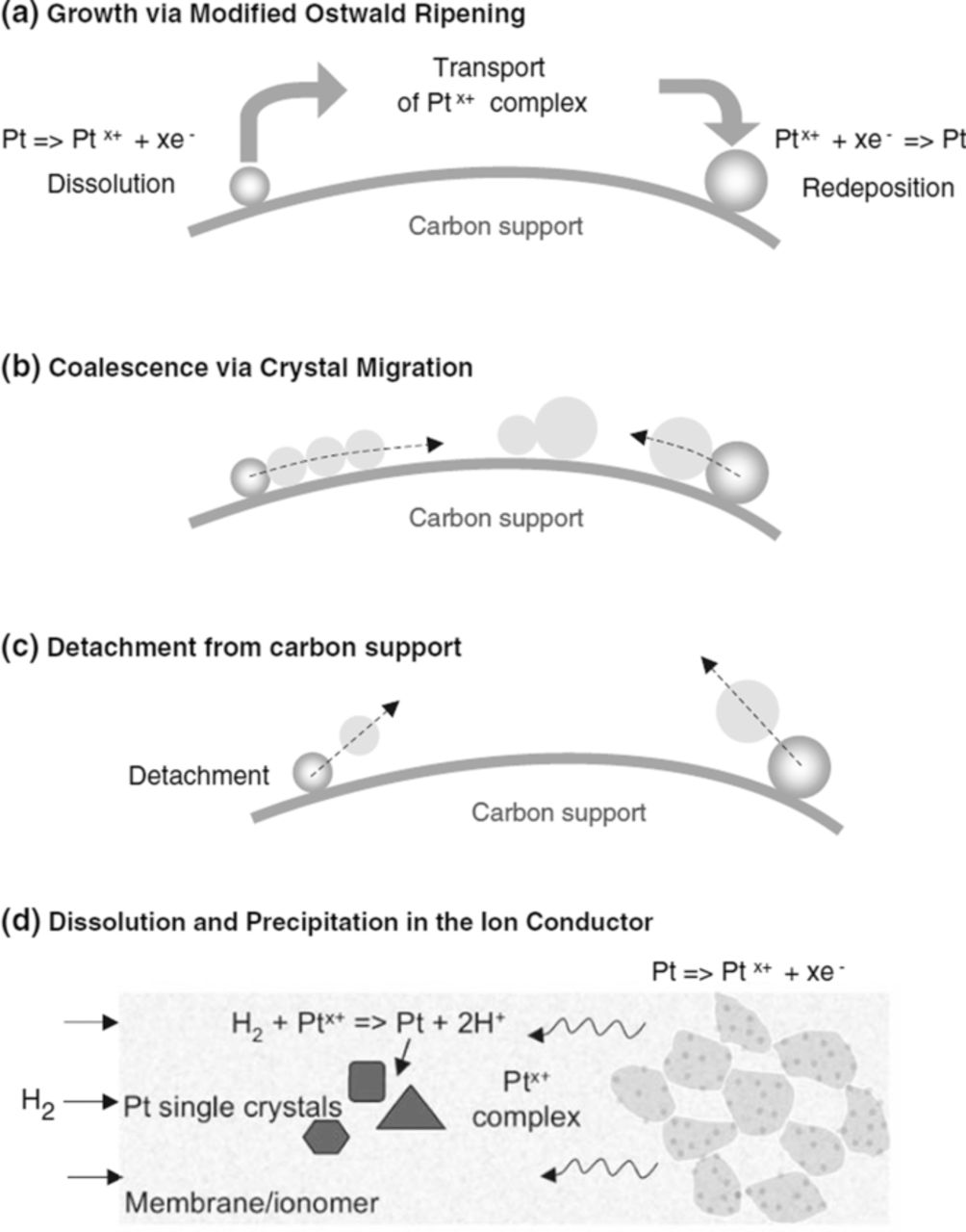
Figure 26. Schematic representation of platinum dissolution and redeposition (image reprinted from Ref. 431 with the kind permission of the publisher).
The mechanism of Pt transport has been primarily shown to be in platinum cations. Both Pt(II) and Pt(IV) species have been detected in a sulfuric solution after potential cycling, and confirmed that the charge difference between anodic and cathodic sweep corresponds with the amount of dissolved species if the upper limit of the potential cycling is chosen to avoid oxygen evolution.436 Pt is transported from the cathode catalyst, and where reprecipitation occurs seems dependent upon operating and transport conditions. Much of the Pt reprecipitates in the cathode catalyst layer creating larger platinum particles as noted in Figure 26 and seen experimentally.437,438 Some of the Pt also reprecipitates in the Nafion membrane, primarily where hydrogen and oxygen diffusion fronts meet and hydrogen reduces the platinum cations creating a 'band' of platinum.439–443 Platinum has also been shown to plate out on the anode catalyst layer/membrane interface.306,320
To describe accurately platinum oxidation and dissolution requires inclusion of anodic and cathodic terms describing both the oxidation and the reduction of platinum oxide to platinum. For example, one can include equilibrium Pt-oxide coverage term in the kinetics (see equations 60 and 61).133,444,445 This coverage is potential dependent and ranges from zero to full coverage, where a full coverage protects the underlying Pt from dissolving even at higher potentials. Thus, one can see the reason why cycling is so detrimental is that one is transitioning to where Pt wants to dissolve thermodynamically and is not yet protected from doing so by the Pt-oxide layer. A more complicated expression can be used for Pt oxide formation, assuming that Pt forms a non-ideal solid solution with the Pt oxides that appear at potentials higher than 0.85 V.426 Thus, the activity of Pt in Pt-PtOx solid solution was derived from experimental dissolution data as
![Equation ([133])](https://content.cld.iop.org/journals/1945-7111/161/12/F1254/revision1/jes_161_12_F1254eqn133.jpg)
where cPt2+ is the concentration of Pt2+ in the perchloric-acid solution. This model was expanded for use on catalyst-coated membranes and related to accelerated stress tests.446 The rate at which Pt dissolves by the reaction Pt = Pt2+ + 2e− is given by
![Equation ([134])](https://content.cld.iop.org/journals/1945-7111/161/12/F1254/revision1/jes_161_12_F1254eqn134.jpg)
This model expansion includes the dynamics of particle-size evolution (dp) considering particle growth by Ostwald ripening and coalescence/sintering. Results from this model indicate that the observed growth in particle size and loss in surface area are primarily due to coalescence/sintering and are sensitive to the potential limits and the initial particle-size distribution. An enthalpy of dissolution of 49.3 kJ.mol−1 and an effective heat of fusion of 28.2 kJ.mol−1 for particle coalescence/sintering have been empirically determined from the measured temperature dependence of particle growth.446 A systematic study is still needed to investigate the effect of O2 on the thermodynamics and kinetics of Pt dissolution in aqueous media. Additionally, the model suggests that a reduction in ionomer hydration limits the diffusion of Pt ions in the ionomer; data is needed to estimate the platinum dissolution rate dependence on ionomer hydration.
As mentioned, Pt ions can move into and across the ionomer, which is a solid acid. This results in deposited particles in the membrane as well as the Pt band mentioned above.434,439–443,447 A substantial amount of Pt can be observed migrating into the membrane induced from potential cycling; measurements have shown up to ∼ 13% 443 to 20%448 of the cathode catalyst-layer Pt deposited into the Nafion membrane. A model based on dilute-solution theory (see equation 28) has been used to describe the movement of soluble platinum through the Nafion membrane.440
There are few publications describing the platinum transport and platinum-dissolution effects on mass-transport limitations in PEFCs, although they seem to indicate larger mass-transfer overpotentials.449
Other restructuring effects
Cathode catalyst-layer thinning is regularly observed and most reports indicate increased losses associated with mass transport.450 This catalyst-layer thinning is coupled with loss of porosity in the catalyst layer, and in some cases correlate with carbon corrosion. It is unclear as to the causes of this catalyst-layer thinning, although restructuring and compaction with an associated loss of porosity of the catalyst layer is suspected. It is also unclear if this effect is widely observed for different MEA manufacturing techniques.
Results have indicated that structural changes in the PEM and catalyst layers are the main reasons for the decline in performance during open-circuit operation as well. The results also show that degradation due to Pt oxidation or catalyst contamination can be partially recovered by a subsequent potential-cycling process, whereas the same cycling process cannot recover the membrane degradation.451 Ionomer degradation in the catalyst layer and membrane have been assumed to be the cause of performance decline during open-circuit-potential holds.418,450
Degradation during freeze/thaw testing have also been attributed to catalyst-layer structural changes and associated with the increased charge transfer and mass-transfer resistances, especially the internal diffusion resistance.178,413,425,452 Related are issues of catalyst-layer delamination, which will impact PEFC performance and transport modeling. To understand these effects, nascent efforts have focused on plasticity and mechanics models of the catalyst layer and its components. The cohesive zone model and the frictional contact model are used to describe the evolution of interfaces between the protonic and the electronic conducting phases.453
Other catalyst-layer effects include dissolution of alloying materials to make platinum alloy. These alloying materials include other noble metals (e.g. Pd, Au, Ir), and metals including Ni, Co, Cr, Fe etc. The leaching effect of these alloying metals on catalyst-layer structure and transport (e.g., in the ionomer thin-film) remains widely unknown to date; most studies have concentrated only on the impact on electrocatalyst kinetics.
Future Perspectives
The above sections outline the critical areas of research and the current progress for continuum-scale modeling of transport in PEFCs. Throughout, not only background and current state of the art is discussed, but critical needs to move the field forward are mentioned. In this section, several of those needs are highlighted and discussed further. In addition, discussion is made on some underlying critical issues for the modeling community including the intersection between the models and experiments, accounted for variations in properties and structures, and the use of open-source modeling.
Intersection with Experiments
As noted throughout this review, the modeling efforts depend heavily on understanding and elucidating the correct physics driving the observed phenomena. In addition, models rely on input parameters of the correct properties, and should be validated by both local and global cell performance and distributions of variables. We believe that to advance the art and understanding of transport modeling requires synergistic efforts in determining effective properties and providing model validation through systematic and orthogonal data sets. In other words, a model should use independently validated submodels or ex- or in-situ measured properties as input parameters, and then be validated in terms of multiple in-operando observations (e.g., water content, response to operation changes, impedance spectra, polarization behavior, etc.), such as that provided at pemfcdata.org. If any fitting parameters are utilized, these should be fit simultaneously to the set of relevant experimental data. In this section, some of the key advances occurring or needed to occur will be highlighted including measurement of effective properties, cell-level studies, and electrochemical impedance spectroscopy.
Effective properties
Recently, there has been a substantial effort to measure directly many of the key transport properties as a function of the various operating conditions such as temperature, pressure, compression, relative humidity, and liquid saturation. Typically, these are measured ex situ, and care must be taken in translating results for complete layers into the discretized modeling domain as mentioned in the multiphase section above. In addition, more sophisticated techniques are being used to validate in situ measurements that were previously accomplished ex situ. For example, recent neutron imaging experiments have confirmed that the measured membrane water content in an operating PEFC is similar to the ex-situ measurements reported over two decades ago.34,61,66 Also, in terms of transport properties, methods have been developed to separate the GDL mass transport from the catalyst-layer transport as well as diffusion mechanisms by varying inlet gas compositions and temperature and total pressure.38,325,454–456
Many of the recent studies have focused on multiphase flow and developing diagnostics to measure effective properties as a function of saturation. For example, one is now using capillary pressure – saturation curves that are measured to calibrate pore-network models that then can simulate different structures and be used for parametric studies, as discussed above. Similarly, there are studies on the perhaps more important variables of breakthrough pressure457–459 and droplet wettability and adhesion, both internally and externally.156,257,460–464 Also, researchers have begun to characterize how the resulting saturation impacts the thermal resistivity. Ex-situ investigations of thermal resistance as a function of saturation have shown that this relationship can be accurately approximated by an effective thermal conductivity.106,465 In terms of oxygen diffusivity, which is a key quantity impacting performance, in-situ characterization has been investigated with AC impedance spectroscopy,466 conductivity cells,41 mercury-intrusion porosimetry,155,467 X-ray computed tomography (XCT),42 Loschmidt diffusion cells,43 and electrochemical techniques.44 As discussed in the empirical-modeling section, Baker et al.38 and Caulk et al.45 established a method and analysis using limiting-current measurements under dry and oversaturated conditions. These limiting current methods and the corresponding analysis have shown that the effective diffusion coefficient follows a characteristic behavior. With increasing current density, a dry then a wet plateau is observed for several types of carbon fiber GDLs.
As discussed in the catalyst-layer section, the catalyst layer is the least characterized of the PEFC components due to the difficulty in measuring its properties. Recent work has concentrated on measuring the properties of the catalyst layers on various polymer, metallic, and non-metallic substrates. The permeability and porosity of a catalyst layer supported on ethylene tetrafluoroethylene has been determined and the catalyst porosity measured using traditional mercury-intrusion porosimetry is lower that what would be expected from typical catalyst layers.468 The water uptake in catalyst layers supported on PTFE membranes has been reported to be lower than that expected from bulk ionomer measurements,157 which directly agree with studies of ionomer thin films as discussed above. The ionic conductivity of PEFC catalyst layers can be directly measured and modeled using AC impedance techniques333 and has been found to be ≈ 100 mΩcm2 in state of the art Pt/C electrodes,333 which is in conflict with some of the thin-film measurements;300,353,358,469 there is no current agreement. The ionic conductivity is a strong function of the Nafion content and needs to be optimized for optimal ionic conductivity and gas transport.470,471
Visualization and validation
The modeling results have traditionally been validated using PEFC performance data, mainly in the form of polarization curves.23,24 However the insensitivity of PEFC polarization curves to varying component materials properties and operating conditions makes model validation a challenge.472 To this end, there is a need for validation through comparison of local variables.
Segmented-cell data has better fidelity than single polarization curves. Segmented cells have been utilized extensively as a diagnostic tool for PEFC as recently reviewed.14,473 The most widely used segmented-cell techniques (commercially available systems) involve segmenting the current collector and measuring the resultant current using printed circuit boards.474–476 There are also several groups that utilize segmented GDLs and even segmented catalyst layers with current being measured either by resistor networks or Hall-effect sensors.477 In addition to measuring current, some systems allow simultaneous measurement of cyclic voltammograms and EIS spectra in each of the segments.
Direct visualization of liquid water in PEFCs is an excellent tool for model validation and significant progress has been made in the past decade in improving visualization techniques.478,479 These techniques include direct optical imaging of specially designed transparent PEFCs,480 X-ray radiography234,240 and tomography,481 neutron scattering,482 radiography,483,484 and tomography,169 and NMR imaging.485 For catalyst layers, while recent work has demonstrated that nano X-ray computed tomography can be utilized to measure their pore distribution,486 it is challenging to obtain the ionomer.487 Scanning transmission x–ray microscopy (STXM),488 scanning electron microscopy331 and other microscopy techniques are being developed to visualize catalyst-layer structures.487 It should also be noted that these techniques normally involve image-based reconstructions of small areas. Thus, there is a need to address the lack of statistic-based variability and the cost/time expense of imaging a sufficient number of samples to attain reproducible results, especially for simulations or validation that depend on them. With the current analysis techniques, the simulation cost from a time perspective is still inherently prohibitive if sample domains approach the scales seen in real PEFC systems. From a validation standpoint, phase resolution in the diagnostic imaging and the use of phase-differentiated distribution data would yield a boon in increasing the confidence in the design capability of these methods.
Amongst the various visualization techniques, the only one capable of imaging water in operando in large-area PEFCs without the need to change MEA, bipolar-plate, and end-plate materials is neutron imaging.479 Although in-plane neutron imaging has been extensively utilized to image water in the PEFC flowfields,489–491 there is not a clear correlation between flowfield water and PEFC performance. The flowfield water observed by neutron imaging has only been successfully correlated to the pressure drop observed and is a useful tool for flowfield and manifold design.491
The resolution of neutron-imaging techniques have improved dramatically over the past decade and high-resolution neutron imaging has been utilized to quantify the through-plane water distribution in PEFCs.66 The advantage of high-resolution through-plane imaging is that it has the potential to provide unambiguously the liquid-water content within the MEA components of an operating PEFCs,160,492–494 and can be utilized to validate PEFC models.66,160 In terms of the last point, Weber and Hickner160 directly compared simulation results to measured water contents, and highlighted PCI flow in the GDLs and discrepancies between the two data sets that still need to be reconciled. Through-plane imaging has also been utilized to demonstrate the water profiles inside the MEAs with different GDL compositions, illustrating the effect of the MPL on cathode-catalyst-layer water content.495 Hussey et al.66 addressed various systematic errors in high-resolution neutron imaging to determine accurately the water content in thick Nafion membranes (up to 1000 μm thick). This work clearly demonstrated that high-resolution neutron imaging can accurately quantify in-situ water content in thicker PEFC components like GDLs and thick membranes. However, the state-of-the-art in imaging still requires improvement in order to quantify catalyst-layer and membrane water content in commercial MEAs.
Electrochemical impedance spectroscopy
Electrochemical impedance spectroscopy (EIS) is a powerful technique used to understand complex phenomena occurring in a PEFC cell. The application of EIS to PEFCs has been illustrated in detail in books,496–498 book chapters,499 and review articles.500 While other techniques are readily modeled with the various modeling equations or derivatives thereof, EIS falls into a special category due to its pervasiveness, ease, and mystery in understanding and interpreting its resulting data, which are compounded by the complexity of the overlapping phenomena.
Impedance spectroscopy is a perturbation technique where a small sinusoidal perturbation during operation allows for the system response to be studied in operando. For example, for a voltage perturbation of the form
![Equation ([135])](https://content.cld.iop.org/journals/1945-7111/161/12/F1254/revision1/jes_161_12_F1254eqn135.jpg)
the current response is phase shifted by φ to be
![Equation ([136])](https://content.cld.iop.org/journals/1945-7111/161/12/F1254/revision1/jes_161_12_F1254eqn136.jpg)
and the frequency-dependent EIS is given in terms of real and imaginary parts
![Equation ([137])](https://content.cld.iop.org/journals/1945-7111/161/12/F1254/revision1/jes_161_12_F1254eqn137.jpg)
The highly non-linear nature of PEFC polarization requires that EIS be performed at various potentials along the polarization curve and then fitted with either an equivalent-circuit model501–503 or more complicated physics-based model.504–507 However, in PEFCs, there are very few publications that use these latter realistic physical models to describe experimental EIS data, and this is a glaring need for the community since EIS is a ubiquitous technique that has the potential to provide a wealth of property and validation data.
To model the impedance, one can follow the methodology of Newman and coworkers.508 From a physics-based model, each of the dependent variable can be written as the sum of its steady-state component (−) and time-varying component (∼) that is frequency dependent,
![Equation ([138])](https://content.cld.iop.org/journals/1945-7111/161/12/F1254/revision1/jes_161_12_F1254eqn138.jpg)
To determine the frequency dependent part of each of the variable, each of the variables is expanded in a Taylor series. Assuming the perturbation is small enough that the system responds linearly, the higher-order terms are neglected,
![Equation ([139])](https://content.cld.iop.org/journals/1945-7111/161/12/F1254/revision1/jes_161_12_F1254eqn139.jpg)
Rewriting the above equations in matrix form to evaluate the unknown frequency dependent terms,
![Equation ([140])](https://content.cld.iop.org/journals/1945-7111/161/12/F1254/revision1/jes_161_12_F1254eqn140.jpg)
Thus, there is only the need to evaluate the time derivative and one can make use of the existing Jacobians to speed up the solution process. From the resulting values, the frequency-dependent EIS is written as the ratio of the frequency-dependent potential and current,
![Equation ([141])](https://content.cld.iop.org/journals/1945-7111/161/12/F1254/revision1/jes_161_12_F1254eqn141.jpg)
By using the governing equations and expressions, one can understand how each variable or property affects the EIS. In terms of computation, the transformations can be done numerically or analytically if possible, and essentially the number of unknowns doubles since each variable now has both a real and an imaginary component.
Overall, EIS is a very powerful experimental tool, especially for characterization and trends, but its results are only as meaningful as the model used for its analysis. Some EIS data is relatively simple to understand such as the high-frequency resistance,509 which is the sum of the membrane resistance, contact resistances, and electronic resistance in the system, and can also be utilized to calculate the membrane-electrode interfacial resistance.223 More complicated analysis arises as one uses EIS to explore the ionic conductivity within the catalyst layer,333,510 334 where the data are often fit using a modified transmission-line model originally proposed by Lefebvre.511 The high-frequency arc in the EIS spectrum consists of a 45o angle line in addition to a capacitive loop and represents the coupled ORR kinetics and catalyst-layer ionic resistance. This high-frequency loop can be modeled to determine the ORR kinetic parameters including exchange current density, Tafel slope and reaction order.512,513 Two Tafel slopes have been observed from the EIS spectra, one at low current densities corresponding to a PtO surface and another at higher current densities corresponding to a reduced Pt surface.514 The EIS results are consistent with the two Tafel-slope model proposed in the literature135 and do not support the single Tafel-slope model.115,121 These EIS measurements assume that the anode reactions are significantly faster than the cathode reactions and the H2 electrode serves as a pseudo reference electrode.
Finally, interpreting the low-frequency part of the EIS response is the most difficult and least understood as it pertains to mass transport and many overlapping phenomena both within the cell sandwich and along the channel.466,504,515 For example, to date, the mass-transfer resistance measured with EIS has not been directly correlated to the saturation measured with visualization techniques. Also, the low-frequency (DC) EIS resistance values are significantly lower than that observed from the slope of the polarization curve at that current density, indicating that a low-frequency inductive loop should be taken into account in any PEFC model that attempts to simulate EIS data.516 Such low-frequency inductive loops have been observed in EIS spectra.333,516 This inductive behavior has been attributed to adsorbed intermediate oxygen species related to the ORR512 or to effects of fluctuating water concentration along the channel.507,517,518 Schneider et al. performed EIS on a segmented cell combined with in-situ neutron imaging and clearly demonstrated the absence of this arc in those sections of the cell that were exposed to liquid water.518 A comprehensive model that takes into account liquid water and is directly able to fit a wide variety of impedance spectra obtained from a cell at different operating conditions is still lacking. However, simpler equivalent-circuit models have been effective in qualitatively correlating mass-transport limitations and providing directions to improve gas transport and PEFC performance.
Modeling Stochastic and Statistical Performance
As discussed in early sections in terms of this review, there is a variability to experiments that should be represented in modeling. For example, freeze kinetics is based on statistical experimental data, as are virtual reconstructions of various cell layers and statistical-based models like pore-network modeling. In addition, experiments also show natural variability due not only to the component variability but also to fluctuations in operating conditions, etc. Models should account for these variations in terms of detailed sensitivity studies, and, for the case of stochastic simulations, an adequate number of virtual experiments or structures.
Given that most of the materials within the MEA present themselves as heterogeneous porous media and that the few that do not still demonstrate variation geometrically from their respective manufacturing processes, it becomes of interest to study the numerical prediction of the cell from a similar statistical basis. This process is relatively straightforward as it is the numerical inputs that are determined prior to a simulation via a statistical selection process. By approaching the inputs in this way, the subsequent simulation represents a "given" configuration out of a batch of N configurations, with N being selected to achieve a desired confidence interval in the performance data. As an example of the type of statistical variation that can be used, Figure 27a shows a typical variation of thickness (geometrical) variation of a GDL as determined by statistical parameters determined from experimental measurement of a batch of GDLs that were to be used in model validation. The figure shows the use of the statistical parameters in creating a "run-to-run" variation of GDL thickness. The use of statistical analysis like this dramatically alters the manner by which a model is said to be validated, as in physical reality one would not achieve a perfect repeat of experimental measured performance curves even if re-testing the exact same PEFC with even greater variation being seen if a similarly configured, but new, PEFC was used.
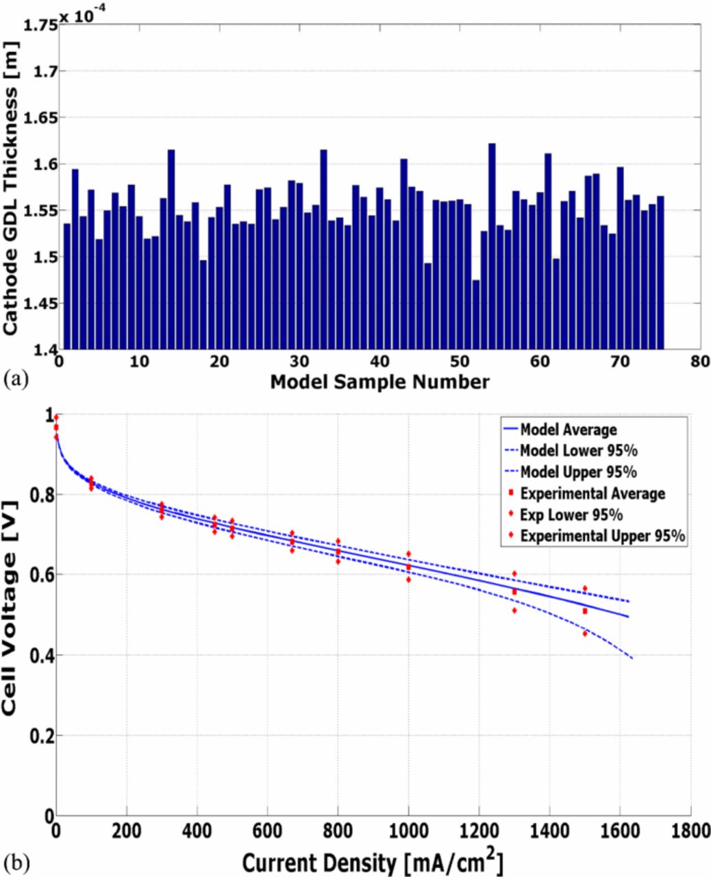
Figure 27. (a) Statistical distribution of GDL thickness as used in a performance model, and (b) statistical validation of a two-phase model using data generated on sample set of 50 similarly composed PEFCs.
Figure 27b shows the results of a validation of a performance model from a statistical basis; from this figure it is interesting to note several aspects. One of the first things is that the statistical variation of the experiment widens as the performance increases, this is of interest as it implies that the cell is becoming increasingly sensitive to various aspects of the material properties or manufacturing variations and that stricter tolerances or controls on the porous-media properties may be required depending on the desired cell operating point. Furthermore, one should also notice that there are combinations of the material characteristics that result in the formation of the characteristic "performance knee" in the 1.2 to 1.4 A/cm2 region where other combinations do not show this and maintain a nearly linear behavior. From the inputs, this aspect seems to be at least in part derived from multiphase flow phenomena. In summary, given the statistical nature of the materials used and the statistical nature of the performance data itself, it becomes apparent that validation of and any information derived from performance or durability simulations should be done using some type of statistical basis.
Open-Source Models
With the advent of open-source publishing and looking toward the future, this section describes the recent efforts for open-source fuel-cell models and also a future outlook of its possibilities. The operation of PEFCs involves many coupled physical phenomena as discussed above, and therefore the development of mathematical physical models is a very challenging endeavor. It is for this reason that over the past two decades there has been tremendous growth on the number and complexity of PEFC models. The majority of PEFC models to date have either been implemented in commercial software such as FLUENT, COMSOL, STAR CD, or implemented in-house. In either case, the source code has not been made available to the public. This has several major drawbacks including:
- Lack of validation and comparison between models. To validate previous models, an independent research group would have to spend a considerable amount of time to re-develop the model. The result is that many of the mathematical models currently in the literature have not been thoroughly validated. Furthermore, most models are not compared to one another.
- Lack of extension capabilities. PEFC mathematical models are constantly evolving. Therefore, previous mathematical models need to be extended to include the most recent understanding of physical processes, such as those discussed above. Only if the source code is available can previous models be extended by other scientists in an efficient and ready manner.
- Implementation limitations. When using commercial software, even if the source code is available, it is not always possible to extend the physics, especially if the partial differential equation does not meet some standard form.
Due to the drawbacks mentioned above, each research group usually re-implements an improved version of the previous mathematical model proposed in the literature, thereby reinventing the wheel and wasting precious time that could be used implementing new features. Furthermore, since each research group includes a modification to the previous model in the literature, and the previous model is not available to the new researchers, mathematical models are not usually compared, thereby making it impossible to assess the impact of the proposed modifications. For example, different versions of the catalyst-layer agglomerate model have been implemented at least a dozen times in the past decade;1,133,281,519–521 however, a detailed comparison between the different models, i.e. using the same geometry and parameters for the different implementations, has yet to be performed.
To enhance collaboration between researchers, several research groups have recently started to share their research source codes, which is believed to be a key future issue/opportunity. To date, there are three known main open-source packages in the literature, i.e. the code developed by Novaresio et al.,522 openFuelCell,523 and openFCST.524 The first two codes focus on solid-oxide fuel cells (SOFCs). The latter focuses on PEFCs and currently contains cathode,279 anode,224 and MEA models and is capable of solving mass and charge transport using Fick's law, Ohm's law, and water transport in the membrane. The code can be used for PEFC analysis, parameter estimation,525 and optimization.526,527 Furthermore, the former two codes are based on the openFOAM finite volume libraries338 while the latter is based on the deal.II finite element libraries .528
The main advantages of developing, sharing and using open-source codes can be summarized as:
- Transparency. Researchers can provide the source code and data files with their articles so that other scientists can verify their results
- Ease to develop new routines by using already existing classes/functions
- Ease to share new developments with the fuel-cell community
- Ease of integration. It is easy to integrate new mathematical models with already existing models in order to develop complex, multi-dimensional fuel cell simulations within a short timeframe
- Easy to validate and compare to previous models
- New models can easily be compared to previously implemented models under the same architecture.
- If a large user base is established, there will be a large number of testers. This would make bugs in the code easy to find.
- It is easy to track and fix bugs. For example, both openFCST and openFuelCell have a ticketing system so that users can submit bugs that were found in the code.
- Ease of integration with other programs. For example, all the open source codes discussed above are integrated with other open-source packages and algorithms such as openFOAM, Trilinos, deal.II, and Dakota.341
The three open-source packages mentioned above were released in 2012 and 2013; therefore, at this point, none of the packages have a large user base. Part of the reason for the slow uptake of open-source codes is that they require a steeper learning curve than commercial software. In the case of in-house codes, the learning curve is worse than open-source packages since most open-source packages provide extensive documentation, e.g., openFCST contains a user guide, a developer guide and a class list reference guide in HTML.524 The key disadvantages of most open-source codes are no graphical user interface and a necessary knowledge of Linux OS and a programming language (preferably an object-oriented language, e.g. C++ or python). To reduce the steep learning curve, most open-source codes have extensive documentation, a mailing list that is used to help new users get started, and many examples.
Due to the advantages of sharing and working together on codes, it is believed that the fuel-cell scientific community could benefit from an open-source framework. The new routines developed by users can be integrated with the current open-source packages thereby leading to the required level of sophistication needed in order to increase our understanding of the physical processes taking place in PEFCs. To overcome the key disadvantages of most open-source packages is to hold trainings and get a buy-in from the community in order to generate a large enough user base. One possible mechanism might be the formation of a clearinghouse where codes can be developed, validated, and enhanced. In this fashion, the main contributing institutions could host a welcome page, the main repository, testing site, and mailing list that all developers submit questions and bugs to in order to ensure a large user base and subsequent quick response times and discussions. In addition, comparison of the simulation results to standard data sets such as the provided at pemfcdata.org using consistent and standard input parameters can provide insights and useful measures of operating ranges and need for better models in terms of properties and phenomena.
As discussed throughout this review, although there are some contentious issues, most of the PEFC physics is becoming standardized. In addition, most PEFC codes are implemented with either a finite-volume or a finite-element analysis library already as a backbone, and thus transitioning to open source may not be too problematic. While full open source is perhaps a good end goal, an intermediate goal of use of a common commercial software package and sharing of the model files could also be a means to bring together the community to build around a single model set. This would not be as easy to modify as open-source code, but it would allow for greater accessibility of the simulations to the larger fuel-cell community, which include the casual modeler. This also alleviates the steep learning curve for open-source codes, especially if the community also provides input into the methods to make the commercial package converge and solve.
Summary and Outlook
Modeling of polymer-electrolyte fuel cells (PEFCs) has advanced significantly over the last couple of decades, where the simultaneous advent of increased computational power and diagnostic techniques have allowed much greater predictability, complexity, and usefulness of the models. Today, design and optimization strategies can be computationally explored with high fidelity and confidence. This critical review has focused on examining these advancements as they relate to modeling of transport phenomena in PEFCs. Throughout, we have discussed the governing phenomena and equations while highlighting the needs and gaps. Of particular focus are issues surrounding multiphase flow and catalyst layers. For the former, there are still unknowns in terms of the correct treatment of interfaces, and, in particular, that with the GDL/gas channel. These interfaces are seen as significantly influencing the overall transport and cell behavior. The land-to-GDL interface is characterized by relatively high ohmic and thermal resistance in conventional channel|land designs, and a location for accumulation of condensing vapor drawn by PCI flow. The channel wall-to-diffusion medium interface has been demonstrated to be a key factor in the retention of water in the DM and cell. The shape and surface condition is important to draw water out of the DM and prevent flooding in the DM. The GDL/MPL interface is a region that has so far been studied the least, with properties that are influenced by the manufacturing method and degree of co-mingling of the layer material. Particularly at the micrometer-scale, more work needs to be done to improve our overall understanding of the interfaces, so that all relevant effects can be included in state-of-the-art multiphase models.
For catalyst layers, there is a need to correlate better the phenomena at the local scale where ionomer thin-films or lack thereof impact performance with the phenomena at the macroscale and thus be predictive. For example, due to the heterogeneous porous structure of the catalyst layer, it is important to establish accurate correlations between the catalyst-layer ionomer and thin-films of ionomer on substrates. It is particularly critical to understand how catalyst-layer properties including, but not limited to, ionomer content, I/C loading, Pt loading, porosity could be studied in thin-film model systems using parameters such as film thickness, substrate/film interactions, film casting and processing. Similarly, one needs to understand how processing conditions, such as hot pressing, can impact overall transport properties and behavior of the ionomer and catalyst layer.
As discussed throughout, there is still a need to link the macroscopic observables and equations with those at smaller length scales in order to provide a truly representative simulation. While such linkages are typically accomplished by transfer of properties, adaptive mechanisms and bidirectional coupling and multiscaling provide still new opportunities and challenges for modeling transport in PEFCs. Virtual or image reconstructions may allow for such a route, but there is still a need for better resolution and more knowledge of the interrelated conditions and formation rules, especially for catalyst layers.
Other transport modeling challenges remain. For example, one needs to understand the sensitivity of the various input parameters (e.g., transport properties) whether they come from experiment or lower-scale models. By knowing the sensitivity, we can see how that matches with experimental results and also provide direction to future activities and research areas. Similarly, this can help to link the modeling results with real-world results in which the systems are much more dynamic with nonuniform properties and stressors. Similarly, one needs to analyze and understand the impact of defects and significant spatial variation in properties that can impact overall performance and durability. This is something that has only minimally been studied in the modeling literature.529,530
In the same fashion, in order to accelerate the components development it is necessary to correlate the measurable properties to the performance effect on a PEFC over its lifetime. This is a place where modeling has a possible significant role to play, since experiments require substantial times to enact. Also, the use of accelerated stress tests and their applicability to real-world and in-operando conditions can be correlated through validated cell models. The issue of lifetime predictions dovetails into that of durability modeling, where there is substantial room for improvement and understanding. While there are some degradation specific models for phenomena as discussed such as catalyst dissolution, a majority of models just alter their transport or related (e.g., water-uptake isotherm or capillary pressure – saturation relationship) properties as a function of time. This method is similar to the use of a fitting parameter with time, and more in-depth modeling and knowledge of degradation phenomena are required to increase the usefulness of macroscopic modeling for durability as it is already for performance.
Overall, significant progress has been made and consensus is being reached for the general treatments and governing equations for modeling transport phenomena in PEFCs. However, as highlighted in this critical review, there are still some significant issues that require more research and understanding. As modeling becomes more common, there is a need to ensure that the proper physics is elucidated and considered, and new modeling methodologies, treatments, and emphasis guided to the key issues.
Acknowledgments
This review has stemmed out of various discussions within and among the members and meetings of the Transport Modeling Working Group of the U.S. Department of Energy, Energy Efficiency and Renewable Energy, Fuel Cell Technologies Office. We thank the program manager Dimitrios Papageorgopoulos for his support, and the financial support of that office to LBNL under contract No. DE-AC02–05CH11231. In addition, we thank those that helped to form this manuscript including Jeff Allen, Sirivatch Shimpalee, and John Van Zee. Finally, we thank the reviewers for their helpful guidance and input, Thomas Fuller, John Weidner, and JES for their support, encouragement, and guidance in writing this critical review.