Glass formers display universal non-equilibrium dynamics on the level of single-particle jumps

When a liquid is cooled to low temperatures and crystallization is avoided (either by a fast cooling rate or due to internal constraints), a glass forms. During cooling, a strong increase in viscosity and relaxation times is observed already in the supercooled regime above the glass transition temperature ${T_\text{g}}$ [1–7]. Based on the temperature dependence of the relaxation times, glass formers are divided into strong and fragile glass formers with strong glass formers displaying Arrhenius and fragile glass formers super-Arrhenius behavior [1]. On cooling through ${T_\text{g}}$ the structural relaxation time, i.e. the time necessary to return to equilibrium after a small perturbation [2], exceeds the time scales accessible in experiments. The glass thus "falls out of equilibrium" rendering it an inherently non-equilibrium system, slowly evolving towards its equilibrium state in a process called "physical aging" [8]. Within the aging regime, dynamic observables depend on the history of the system, i.e. the time since vitrification as well as details of the quenching procedure such as the cooling rate. This history dependence effectively hinders a direct comparison of the non-equilibrium dynamics of different glass formers or glasses with different histories.

In numerical simulations the accessible time scales are many orders of magnitude smaller than in real-world experiments (typically about 100 ns). Thus, the relaxation times reach the accessible time scales already in the supercooled regime around ${T_\text{c}}$, the extrapolated critical temperature of mode coupling theory [1,4,5,7]. Still, non-equilibrium effects can be removed by extensive tempering at these temperatures and relaxation toward equilibrium can be achieved. It has been suggested, however, that this prolonged equilibration dynamics displays the same characteristics as physical aging below ${T_\text{g}}$ [9].

While being restricted to short time scales, numerical simulations offer the benefit that the full microscopic information is available. In this way, computer simulations have played a pivotal role in the understanding of glasses, revealing the presence of increasingly complex dynamics upon cooling, evident in strong spatial correlations [1,3,10,11] and dynamic heterogeneities, i.e. the coexistence of "fast" and "slow" particles [1–3,12–18]. Furthermore, a careful analysis of the single-particle trajectories led to the observation that a facet of dynamic heterogeneities manifests itself in long periods of localized motion interrupted by fast jumps [1,19–22]. Inspired by this observation, glass-forming materials have been studied in terms of the continuous-time random walk (CTRW) [23–27], i.e. a random walk with random time intervals between steps. The CTRW has inspired both theoretical models [19,28–31] as well as the analysis of numerical simulations in various glass formers, including binary mixtures [20,22,32–37], molecular liquids [38], polymers [20,22,39–44], amorphous silica [21,33] and colloids [45].

The CTRW description of glass dynamics hinges on two assumptions: 1) Particles may be considered as individual, non-interacting random walkers on the level of single-particle jumps. This assumption implies that the potential-energy landscape (PEL) of the full system can be separated into (effective) PELs for all individual particles. 2) Jumps are renewal events, i.e. the dynamics following a jump is independent from the history of the process. Thus, the PEL does not change during aging. In this picture aging is a purely stochastic process during which the particles explore deeper and deeper minima, leading to a slowing down of the dynamics. It is not obvious that these assumptions should hold in a molecular system. In fact, considering the increasing density during aging and dynamic facilitation, it would seem more plausible to assume otherwise.

The following analysis may thus be regarded as a test of the assumptions stated above: We study the relaxation dynamics in the supercooled regime around ${T_\text{c}}$. Using the CTRW theory, we derive an analytic expression for the jump or relaxation rate, a property which is particularly suitable as it depends only on the time evolution of the CTRW and compare it to simulations of amorphous silica and a polymer melt as representatives of strong and fragile glass formers. We find good agreement between theory and simulations, which confirms the applicability of the CTRW approach and highlights the universal dynamics on the level of single-particle jumps.

First, let us focus on the CTRW prediction for the jump rate to which we want to compare the simulation results later on. In contrast to a standard random walk, the CTRW assumes random time intervals between the steps. These waiting times ${\tau}$ are assumed to be independent random variables, distributed according to the waiting time distribution (WTD) ${\psi}({\tau})$. This central property governs the time evolution of the CTRW and is the starting point of our analysis. It has been suggested that the WTD for single-particle jumps in supercooled liquids is well described by a Gamma distribution [38,43,45]

$$\begin{equation} {\psi}(t)= A\,t^{\alpha-1}\text{e}^{-\lambda t}, \end{equation} \tag{ 1 }$$

where $0<\alpha\leq1$ and the normalization constant $A=\lambda^{\alpha}/\Gamma (\alpha)$ with $\Gamma(x)$ being the Gamma function. The Gamma distribution displays a power-law behavior at short times $t\ll\lambda^{-1}$ and an exponential decay at late times $t\gg\lambda^{-1}$ (see footnote ¹ ).

From the WTD the jump rate can be derived as follows: The probability that the n-th jump takes place at time t is given by the convolution [27]

$$\begin{equation} {p}_{n}(t)=\int_{0}^{t}{p}_{n-1}(t_{n-1}){\psi} (t-t_{n-1})\,{\text{d}} t_{n-1}. \end{equation} \tag{ 2 }$$

Equation (2) states that the n-th jump takes place at time t if the previous jump took place at time $t_{n-1}$ and was followed by a waiting time of $t-t_{n-1}$. The convolution is calculated over all accessible times $t_{n-1}$. The jump rate is then the probability that a jump with arbitrary n takes place at time t.

$$\begin{equation} {\nu}(t)=\sum_{n=1}^{\infty}{p}_{n}(t). \end{equation} \tag{ 3 }$$

Under Laplace transform it is given by

$$\begin{equation} {{\mathcal{L}\left\{{{\nu}(t)}\right\}}}=\tilde{{\nu}}(s) =\sum_{n=1}^{\infty}\tilde{{p}}_{n}(s)=\sum_{n=1}^{\infty}\tilde{{ \psi}}_{1}(s)\tilde{{\psi}}(s)^{n-1}, \end{equation} \tag{ 4 }$$

where the persistence time distribution (PTD) ${\psi_{1}}(t)$ is the distribution of times between the start of the observation and the first jump. This distribution differs in general from the WTD and is, furthermore, subject to aging [27,46]. The difference between the PTD and the WTD can be illustrated by the trap model [30]. In this model the particles traverse a series of traps of varying depth. Thus, the WTD is determined by the distribution of available traps, whereas the PTD is determined by the distribution of occupied traps. An often made assumption is that at time t = 0 all traps are occupied with the same probability, i.e. ${\psi_{1}}\equiv{\psi}$. This state corresponds to a quench from a very high temperature and can be identified with the age zero. During aging, the particles tend to accumulate in deeper and deeper traps, leading to an age-dependent PTD and a slowing down of the dynamics. When equilibrium is reached, the PTD takes the form [27,43,47]

$$\begin{equation} {\psi_{1}}({\tau_{1}})=\frac{1}{\langle{\tau}\rangle} \int_{{\tau_{1}}}^{\infty}{\psi}({\tau})\;\mathrm{d} {\tau}. \end{equation} \tag{ 5 }$$

Thus, the PTD contains the full history dependence of the process. For the following steps, we assume ${\psi_{1}}\equiv{\psi}$ and discuss this assumption below in view of the analysis of the simulation data. Then, the jump rate is given by

$$\begin{equation} \tilde{{\nu}}(s)=\frac{\tilde{{\psi}}(s)}{1-\tilde{{ \psi}}(s)}. \end{equation} \tag{ 6 }$$

We can now insert into this general expression the Laplace transform of the Gamma distribution $\tilde{{\psi}}(s)=\lambda^{\alpha}\left(\lambda+s\right) ^{-\alpha}$. Transforming back we find

$$\begin{equation} {\nu}(t)=\lambda^{\alpha}e^{-\lambda t}t^{\alpha-1}\mathrm{E}_{\alpha, \alpha}\left[(\lambda t)^{\alpha}\right], \end{equation} \tag{ 7 }$$

where $\mathrm{E}_{\alpha,\beta}(z)=\sum_{k=0}^{\infty}z^{k}/\Gamma(\alpha k+\beta)$ is the two-parameter Mittag-Leffler function [48,49].

We can use the series expansion of the Mittag-Leffler function to find an expression for the two limiting cases

$$\begin{equation} {\nu}(t)=\begin{cases} \displaystyle\frac{\lambda^{\alpha}}{\Gamma(\alpha)}t^{\alpha-1}, & \text{ for } t \ll\lambda^{-1},\\ \displaystyle\frac{\lambda}{\alpha}=\frac{1}{\langle{\tau}\rangle}, & \text{ for } t\gg\lambda^{-1}, \end{cases} \end{equation} \tag{ 8 }$$

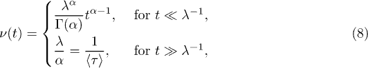
where $\langle{\tau}\rangle=\int_{0}^{\infty}t{\psi}(t) {\text{d}}t=\alpha\lambda^{-1}$ is the mean waiting time. The CTRW theory thus predicts a power-law decay of the jump rate, which turns into a constant rate when equilibrium is attained. This describes the qualitative behavior of the jump rate reported in the literature [21,41].

We compared the analytic expression for the jump rate, eq. (7), to molecular-dynamics (MD) simulations of glass-forming liquids. To this end, we analyzed jump events in amorphous silica $(\text{SiO}_{2})$ [21] and in a short-chain polymer melt [42], which are typical representatives of strong and fragile glass formers, respectively. Particle interactions in amorphous silica were modeled by the Beest-Kramer-van Santen (BKS) potential [50] with slightly modified parameters (see [9] for details). A fully equilibrated configuration consisting of 112 Si and 224 O particles was quenched instantaneously from the initial temperature ${T_{\text{i}}}=5000\ \text{K}$ to one of the final temperatures ${T_{\text{f}}}\in\{2750\ \text{K},\,3000\ \text{K},\,3250\ \text{K}\}$ (${T_\text{c}} = 3330\ \text{K}$ [51])² . For each value of ${T_{\text{f}}}$, 20 independent configurations have been simulated for 33 ns. For the fragile glass former, a generic bead-spring polymer model [42,43,52] was employed. Simulations of a bulk polymer melt of 3072 polymers with N = 4 monomers each were performed. Four fully equilibrated systems at $T=0.37$, 0.38, 0.39 and 0.40 ($T_{\text{c}}= 0.383$ [52]) with pressure p = 0 have been considered. The lengths of the analysed trajectories were $2.2\cdot10^{6}$ for $T=0.37$, $1\cdot10^{6}$ for $T=0.38$, $1.2\cdot10^{6}$ for $T=0.39$ and $2\cdot10^{5}$ for $T=0.40$. For the polymer model, all quantities are given in Lennard-Jones units. Note that these systems are significantly different: The amorphous silica is a strong glass former out of equilibrium, while the polymer model is a fragile glass former in equilibrium. Using standard techniques it would thus be impossible to directly compare the dynamics. It is, however, feasible using the method proposed here.

For the jump detection single-particle trajectories were discretized into time windows of size $\Delta t$ and for each time window the average positions $\overline{\boldsymbol{r}}_{n}(t_{l})$ and the fluctuations $\sigma_{n}(t_{l})=\sqrt{ \overline{\boldsymbol{r}^{2}_{n}}(t_{l})-\overline{\boldsymbol{r}}^{2}_{n}(t_{l})}$ were determined, where the index l denotes the time window. We labeled particle n as "moving" if its change in average position $\Delta\overline{\boldsymbol{r}}_{n}=| \overline{\boldsymbol{r}}_{n}(t_{l})-\overline{\boldsymbol{r}}_{n}(t_{l-\delta})|>3\langle\sigma \rangle$ with $\delta=2$ for the polymer melt and $\delta=4$ for the amorphous silica. The product $\delta\cdot\Delta t$ determines the resolution of the jump detection. It should be as small as possible yet large enough to fully encompass the jumps. We discuss below the effect of the finite resolution and how it was accounted for. For the amorphous silica 〈σ〉 is the average fluctuation where time windows during which jumps occur have been excluded [21]. For the polymer melt, $\langle\sigma\rangle=0.155$ was determined at $T= 0.39$ [42] and this value was fixed for all temperatures. By comparing 〈σ〉 to the position of the first peak in the radial distribution function [52,53] we have confirmed that 〈σ〉 is of the same order of magnitude both for amorphous silica and the polymer model. Note that this jump-detection method differs from the one applied to the polymer melt in [42]. We have compared the method applied here to the one of [42] to confirm that the detection method does not have an impact on the results. In a further step a refinement procedure was employed to filter out strongly correlated moves. The resulting subset of moves constitute the "jumps" which will be analyzed in the following. The refinement methods for silica and the polymer model differ and have been discussed in [21] and [42], respectively. It has been shown for the polymer melt that the jumps fulfill the conditions of a CTRW to a great extent, i.e. that no correlations between waiting times exist [42] and that the WTD does not depend on the history of the process [44]. Using the method suggested in [44] we have confirmed that the same applies to the jumps detected in $\text{SiO}_{2}$.

For the further analysis, it is important to consider the finite resolution of the jump detection. The jump detection in MD simulations relies on a coarse graining of single-particle trajectories. Thus, two jumps need to be separated by a minimum waiting time of ${\tau_{\min}}$, where ${\tau_{\min}}= 0.02616\ \text{ns}$ for the amorphous silica [21] and ${\tau_{\min}}= 100$ for the polymer model [42]. Comparing ${\tau_{\min}}$ to $\tau_{\text{cage}}$, i.e. the time where the incoherent scattering function and the mean-square displacement reach their plateau value, we have confirmed that ${\tau_{\min}}$ is of the same order of magnitude for amorphous silica and the polymer model. This cutoff at short times implies that the WTD vanishes for ${\tau}<{\tau _{\min}}$, yielding the effective mean waiting time

$$\begin{equation} \langle{\tau}\rangle_{\text{eff}}=\int_{{\tau_{\min}}}^{\infty} t{\psi}(t)\,\mathrm{d}t=\frac{\Gamma(\alpha+1,\lambda\,{ \tau_{\min}})}{\lambda\,\Gamma(\alpha,\lambda\,{\tau_{\min}})}, \end{equation} \tag{ 9 }$$

where eq. (1) was used and $\Gamma(s,x)$ is the upper incomplete Gamma function. Note, that the normalization factor in eq. (1) changes to $A = \lambda^{\alpha}/\Gamma(\alpha,\lambda{\tau_{\min}})$ if all waiting times ${\tau}<{\tau_{\min}}$ are omitted. The effect of the lower cutoff can, in good approximation, be accounted for by multiplying the jump rate in eq. (7) with $\alpha\lambda^{-1}\langle {\tau}\rangle^{-1}_{\text{eff}}$. We have performed CTRW simulations [43] to confirm that this approximation is valid within the parameter range found in the MD simulations³ .

In eq. (6) we assumed ${\psi_{1}}\equiv {\psi}$. This is, however, not the case for jumps detected in a supercooled liquid or glass. Instead, the PTD depends strongly on the history of the process, i.e. on the quench protocol and on the age of the system [20]. It is thus not possible to directly compare the simulation results with the analytic formula, eq. (7). Instead, we apply the following procedure: We define an internal time $t'$ by setting the internal clock of each particle to zero just after its first jump⁴ . The internal time is thus defined as

$$\begin{equation} t' = t - t_{1,i}, \end{equation} \tag{ 10 }$$

where t_1,i is the first jump time of particle i. In the definition of the internal time, we make use of the second assumption stated in the introduction that jumps are renewal events. The proposed method can be rationalized in terms of dynamic heterogeneities as follows: In supercooled liquids and glasses fast and slow particles coexist and with time fast particles can become slow and vice versa. In the transformation to the internal time, one identifies the new time origin with a period during which the particle is fast. Thus, at $t' = 0$ all particles are fast. During the time evolution, more and more particles return to a slow state, leading to a slowing down of the dynamics in the internal time. The such prepared initial state is a well-defined out-of-equilibrium state, independent of the history of the system. Hence, the single-particle dynamics in the internal time are identical, irrespectively of whether the trajectories were recorded in an aging system (as is the case for the amorphous silica) or in an equilibrium melt (as for the polymer). Note that the so-prepared state exactly corresponds to the initial state used in the derivation of eq. (7), defined via ${\psi_{1}}\equiv {\psi}$. The jump rate in the internal time is calculated as

$$\begin{equation} {\nu}(t')=\frac{1}{N_{\text{p}}\Delta t}\sum_{i=0}^{N_{\text{p}}} I_{i}(t'), \end{equation} \tag{ 11 }$$

where $N_{\text{p}}$ is the total number of particles, $\Delta t$ the size of a time window and $I_{i}(t') = 1$ if particle i jumps in the time window corresponding to time $t'$ and zero otherwise.

To compare eq. (7) to the MD simulations, first the parameters α and λ need to be determined. To this end, the WTD was recorded and the data were fitted to eq. (1). The observed WTDs for the fragile and strong glass former are displayed in fig. 1. The fit results are listed in table 1. Then, eq. (7) was used to determine ${\nu}(t')$ numerically [54]. The jump rate obtained from the MD simulations, eq. (11), is in very good agreement with the analytic expression, eq. (7), as shown in fig. 2. Only small deviations are visible for the silica model at the highest temperature which we attribute to the short power-law regime available for the determination of the parameter α. Due to this good agreement, we can infer that the assumptions stated in the introduction are indeed valid on the level of single-particle jumps.

Table 1:.  Parameters α and λ obtained via least-square fit of the WTD (see fig. 1) to eq. (1). Note that these values differ from the values reported in [21,42] where the WTD was fitted with a single power law.

Polymer
T	0.37	0.38	0.39	0.40
α	0.194	0.279	0.338	0.420
λ	$5.46\cdot 10^{-6}$	$1.86\cdot 10^{-5}$	$5.31\cdot 10^{-5}$	$1.57\cdot 10^{-4}$

	Silica
T	2750 K	3000 K	3250 K
α	0.21	0.38	0.58
λ	0.060	0.37	1.66

Zoom In Zoom Out Reset image size

Figure 2, furthermore, highlights the remarkable observation that strong and fragile glass formers display universal dynamics for single-particle jumps [19]. Thus, it allows a direct comparison of the non-equilibrium dynamics of different glass formers despite their different quench protocols. For example, the value of α is almost identical for oxygen atoms in amorphous silica at $T = 3000\ \text{K}$ and monomers in a short-chain polymer melt at $T = 0.39$. The same holds for oxygen atoms at $T = 2750$ and monomers at $T = 0.37$. The jump rates would thus overlap when the time is scaled by λ.

It is important to note that the time $t'$ in fig. 2 does not correspond to the external, physical time, but to the internal time defined via eq. (10). The jump rate in the internal time can thus be regarded as the single-particle picture of dynamic heterogeneities: Directly after a jump (corresponding to the jump at $t' = 0$), the particles have an increased probability of performing further jumps shortly thereafter, rendering the particle fast. This agrees with the observation in ref. [19] that a particle, which performs a jump, will likely perform one or several further jumps during the observation. In [19] the WTD is modeled by an exponential. Such a modeling, however, would lead to a time-independent jump rate and would thus not allow an initial fast particle (at $t' = 0$) to "slow down" toward the average behavior, given by the large-t limit of eq. (8). In contrast, the Gamma distribution is capable of describing this crossover.

Zoom In Zoom Out Reset image size

Another conclusion that can be drawn from fig. 2 is that the time $t = \lambda^{-1}$ marks the transition from non-equilibrium to equilibrium dynamics. The characteristic time scale of the exponential cutoff in the WTD can thus be identified with the equilibration time $t_{\text{eq}}$. Comparing $\lambda^{-1}$ for the silica melt with the equilibration time t₂₃ from ref. [9] we find that $\lambda^{-1}$ is of the same order of magnitude as t₂₃, albeit by a factor of 2 to 6 larger. The parameter λ, furthermore, dominates the slowing down of the dynamics on approaching ${T_\text{g}}$ [22], and is thus of particular interest. To determine λ from the WTD, however, the observation time needs to be of the same order of magnitude as $\lambda^{-1}$. On the other hand, λ has a strong influence already on the short-time behavior of the jump rate, as can be seen from eq. (8). Thus, it is possible to extrapolate the equilibration time from the jump rate long before the system actually reaches equilibrium. To this end, first the parameter α should be obtained from the WTD using a power-law fit. Then, the value of λ can be obtained by fitting the jump rate to eq. (7). We have performed these steps for the polymer model at $T = 0.37$ using only data for $t' < 10^{3}$, finding $\lambda = (3.8 \pm 0.3)10^{-6}$. Similarly, we found $\lambda = (0.049 \pm 0.004)$ for the amorphous silica at $T = 2750\ \text{K}$ using only data for $t' < 0.2\ \text{ns}$. These values are very close to the correct values $5.46\cdot 10^{-6}$ and 0.06, even though the fit range is in both cases about two orders of magnitude smaller than $\lambda^{-1}$.

It is interesting to note that while the jump rate is well suited to determine the parameter λ, the influence of the parameter α is hardly discernible. In fact, displaying $\langle{\tau}\rangle_{\text{eff}}\; {\nu} (\lambda t')$ we find that all data superimpose.

In summary, we found an analytic expression for the relaxation rate in non-equilibrium glass-forming liquids, eq. (7), based on the assumption that relaxation events can be identified with "jumps" of a CTRW. This assumption is not obvious to hold a priori, as it implies that the dynamics following a jump is independent of the history of the system, i.e. identical irrespectively of whether the jumps have been recorded in a non-equilibrium aging system or in an equilibrium melt. Comparison of eq. (7) to MD simulations of both a strong and fragile glass former in the supercooled regime, however, yields very good agreement. The results discussed here indicate that the CTRW provides a suitable framework for the analysis of the single-particle dynamics in glass-forming materials, allowing the non-equilibrium dynamics of very different glass formers to be compared directly. Additionally, our analysis suggests that the equilibration time can be determined from the jump rate already for relatively short trajectories. The results could prove helpful in the analysis of the dynamics in systems far below the glass transition temperature and systems under physical deformation and of mechanical rejuvenation.

JH is indebted to A. Blumen and F. Thiel for helpful discussions as well as to S. Frey for preparation of the equilibrium configurations and O. Benzerara for assistance in the numerical simulations. We greatly acknowledge financial support from the IRTG "Soft Matter Science", the DFH/UFA and the Marie Curie International Research Staff Exchange Scheme Fellowship within the 7th European Community Framework Program SPIDER (PIRSES-GA-2011-295302). Parts of this work have been performed in Lviv, Ukraine.