Abstract
This article describes the optimization of processing parameters for the surface roughness of AISI316 austenitic stainless steel. While experimenting, parameters in the process like feed rate (fd), speed (vc), and depth of cut (DoC) were used to study the outcome on the surface roughness (Ra) of the workpiece. The experiment was carried out using the design of experiments (DOE) on a computer numerical control (CNC) lathe. The surface roughness is tested for three conditions i.e. Dry, Wet, and cryogenic conditions after the turning process. Samples are step turned on CNC Lathe for all three conditions with a set of experiments designed. The response surface methodology is implemented, and mathematical models are built for all three conditions. The nature-inspired algorithm is the best way to get the optimal value. For the discussed problem in the paper, nature-inspired techniques are used for obtaining the optimum parameter values to get minimum surface roughness for all set conditions. The Grasshopper optimization algorithm (GOA) is the technique that is the most effective method for real-life applications. In this research, GOA is used to get optimum values for the surface roughness (Ra) at Dry, Wet and cryogenic conditions. Finally, results are compared, and it's observed that the values obtained from GOA are minimum in surface roughness value.
1. Introduction
Stainless steel is also called corrosion resilient steel due to iron-based steel alloy with a least chromium content of 11 %. Stainless steel normally has weldability, high ductility, and low-temperature toughness. Stainless steel has many uses in construction, transportation, chemical or pharmaceutical, offshore oil and gas pipelines, food and beverages, hot water tanks and springs, fasteners (bolts, nuts and washers), metal wires and more [1, 2]. As AISI 316 austenitic stainless-steel material needs to be machined, it is necessary to study the influence of machining (turning) on the surface finish and the cutting tool. Surface finish is a vital part of machined products [3, 4].
Youssef Touggui et al. [5] studied various parameters affecting material removal rate and surface roughness on AISI 316 in turning operation. The parameters considered were speed, feed and depth of cut in the research study. The problem considered was to maximize material removal rate and minimize the surface roughness at a time. Tze Chuen Yap [6] investigated role of cryogenic cooling in metals. And also studied and presented the cryogenic cooling effect on turning of different metals and alloys. Muhammmad Yasir et. al. [7] researched on effect of cutting speed and feed rate on surface roughness of AISI 316l. The focus of their study was to find out the effect on surface roughness with respect to different parameters. After observing the different literature, it observed that the surface roughness depends on cutting speed and feed and depth of cut. The cutting environment also affects the tool and workpiece.
In this work, we considered the influence/effect of processing parameters. The effect on surface roughness of three processing parameters was considered i.e., feed rate, speed, and depth of cut and three different conditions were considered i.e., dry, wet and cryogenic. Dry condition refers to turning the workpiece without any coolant usage wet condition refers to using a coolant while turning process and cryogenic condition refers to cooling the workpiece with socking time and then performing the turning process. Taguchi Design is used to determine the best machining parameter settings for the selected tool/workpiece combination under dry, wet and cryogenic conditions to minimize surface roughness [8, 9]. AISI 316 Austenitic Stainless-Steel material is selected as a workpiece material for studying a machining process (turning process) at different selected cutting environmental conditions varying selected cutting parameters. Samples are step turned on CNC Lathe for all three conditions with a set of experiments designed. The response surface methodology is implemented, and mathematical models are built for all three conditions.
Nature-inspired and Bio-inspired algorithms nowadays play a very vital role in the optimization of the process parameters or in solving real-life problems. There are many such algorithms which can be listed as Genetic algorithm (GA) [10], Particle Swarm Optimization (PSO) [11], Grey Wolf Algorithm (GWA) [12], Cuckoo Search Algorithm (CS) [13], Bat Algorithm (BA) [14], Salp Swarm Algorithm (SSA) [15], Firefly Algorithm (FA) [16], Flower Pollination Algorithm (FPA) [17] etc. also there are algorithms like Socio inspired algorithms which are on the social behaviour of human beings such as Cohort Intelligence Algorithm (CI) [18], Ideology Algorithm (IA) [19] etc. One such algorithm is known as the Grasshopper optimization algorithm (GOA) [20, 21] is used in this research to get optimum value or the best combination of speed, feed and depth for dry, wet and cryogenic cutting conditions.
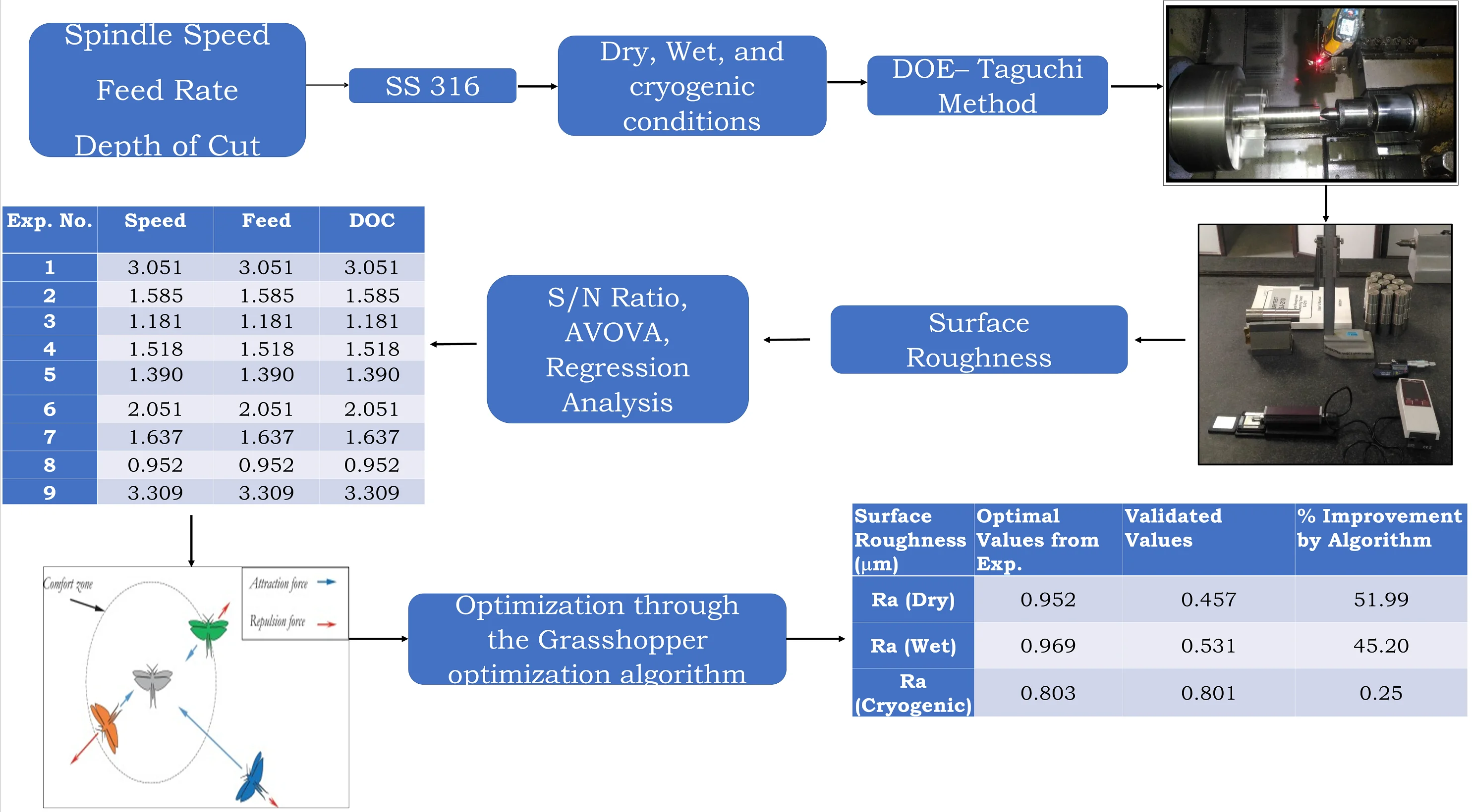
The project aims at the obtaining higher surface finish for material AISI 316 austenitic stainless. The methodology flows as the study of parameters responsible for surface finish. The next step goes in to planning for design of experiments (DOE), performance of experiments followed by linear regression analysis. Then optimizing the parameter responsible for surface roughness with the help of Grasshopper optimization algorithm (GOA). The optimized results obtained from the algorithm are validated and surface roughness is measured which gives a higher surface roughness.
The novelty of this research was that this is the first attempt to use Grasshopper optimization algorithm to optimize surface roughness.
2. Methodology
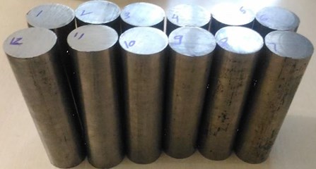
The AISI 316 austenitic stainless-steel material is considered for research after referencing different literature. Table No. 1 shows the chemical properties of AISI 316 material. Table 2 shows the component specification. For the experimentation specific component was manufactured shown in Fig. 1. Cutting tests were performed on a CNC lathe machine under dry, wet and cryogenic machining conditions. The PVD coated carbide insert is suitable for this operation. [22, 23, 24]. The different environmental conditions experimented within this research are dry which is performing turning process without coolant and at ambient temperature, wet which performing experiments with coolant and cryogenic. The coolant used for Wet Turning is ‘GRODAL CUTSOL. A’ coolant Grodal Cutsol A is a high-quality mineral oil containing a cooling lubricant with excellent benefits. Cryogenic machining is a method of cooling the workpiece during material removal processes. The coolant is usually nitrogen fluid (LN) that is liquefied by cooling to –196 °C for 4 Hr. Nitrogen is a safe, non-combustible, and noncorrosive gas. 78 % of the air we breathe is nitrogen.
Table 1Elements in AISI 316 austenitic stainless steel
C | Cr | Ni | Mn | Si | N | S | P | Mo |
0.08 max | 16.00-18.00 | 10.00-14.00 | 2.00 max | 0.75 max | 0.10 max | 0.030 max | 0.045 max | 2.00-3.00 |
Table 2Component specifications
Diameter | 36 mm |
Length | 130 mm |
Material | AISI 316 Austenitic Stainless Steel |
Quantity | Dry No. 9; Wet No. 9; Cryogenic No. 9 |
Fig. 1Workpiece Material AISI 316
2.1. Selecting the parameters for cutting
The range of cutting limits is based on AISI316 austenitic stainless-steel materials and cutting tools used for machining. Factors such as depth of cut, speed and feed are selected as control factors. Each control factor requires three levels. Table 3 lists the factors and levels of process parameters [25-27].
Table 3Factors and levels of process parameters
Levels | Cutting speed () m/min | Feed rate () mm/rev | Depth of cut (d.o.c) (mm) |
1 | 160 | 0.1 | 0.5 |
2 | 180 | 0.2 | 1 |
3 | 200 | 0.3 | 1.5 |
2.2. Design of experiment
“Design of experiments (DOE) is an organized way to establish the association between process-influencing factors and process output. This information is needed to manage process inputs, optimize output, and reduce experiment time. Design of experiments is based on Taguchi’s design technology” [27]. Since each has 3 processing parameters and 3 levels, a 3-level design was selected, as shown in Table 3. Choose the L9 array and get the best combination. Table 4 shows the orthogonal design. The experiment was performed under different environmental conditions, namely dry, wet and cryogenic. The experiment was carried out on the FANUC series Oi Mate-TC CNC lathe as shown in Fig. 2. Therefore, in all 9 experiments with 3 different conditions we performed so in all 27 experiments were performed.
Fig. 2CNC machine
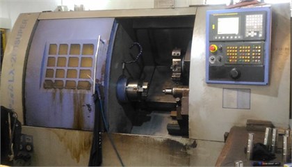
Table 4L9 orthogonal design matrix
Sr. No. | Cutting speed () m/min | Feed rate () mm/rev | Depth of cut (d.o.c) (mm) |
1 | 160 | 0.2 | 1.5 |
2 | 160 | 0.1 | 1 |
3 | 160 | 0.3 | 0.5 |
4 | 180 | 0.3 | 1.5 |
5 | 180 | 0.2 | 1 |
6 | 180 | 0.1 | 0.5 |
7 | 200 | 0.1 | 1.5 |
8 | 200 | 0.3 | 1 |
9 | 200 | 0.2 | 0.5 |
3. Results with discussion
3.1. Surface roughness
The measurement of surface roughness was carried out with the help of Surface Roughness Measuring Tester SJ-210. The measurement was taken at three instants on the machined surface and then the average surface roughness value was taken. Table 5 shows the average values of at dry, wet and cryogenic cutting conditions.
Table 5Surface roughness values for dry, wet and cryogenic machining
Expt No. | (m/min) | (mm/rev) | d.o.c. (mm) | Average value of 3 location (μm) | ||
Ra (Dry) | Ra (Wet) | Ra (Cryogenic) | ||||
1 | 160 | 0.2 | 1.5 | 3.051 | 1.653 | 1.621 |
2 | 160 | 0.1 | 1 | 1.585 | 3.411 | 1.068 |
3 | 160 | 0.3 | 0.5 | 1.181 | 1.257 | 3.311 |
4 | 180 | 0.3 | 1.5 | 1.518 | 1.635 | 3.169 |
5 | 180 | 0.2 | 1 | 1.390 | 3.220 | 1.755 |
6 | 180 | 0.1 | 0.5 | 2.051 | 1.152 | 0.803 |
7 | 200 | 0.1 | 1.5 | 1.637 | 3.064 | 1.153 |
8 | 200 | 0.3 | 1 | 0.952 | 1.681 | 3.248 |
9 | 200 | 0.2 | 0.5 | 3.309 | 0.969 | 1.697 |
From Table 5, it is seen that the minimum surface roughness values for dry machining are achieved by experiment 8 which is 0.952 μm. In wet machining, the minimum value of surface roughness is 0.969 μm achieved through the 9th experiment. In cryogenic machining, the surface roughness value is 0.803 μm achieved in expt. No. 6.
3.2. Analysis of DoE
The purpose of this work is to obtain a comprehensive optimized value of surface roughness. Three process parameters have been selected, and each of the three levels has flipped the selected material. Depth of cut, speed and feed rate are regarded as turning process parameters. Since we have to minimize the surface roughness value, the S/N ratio is used for minimization. Tables 6, 7 and 8 show the response table of the signal-to-noise ratio under dry, wet, and cryogenic conditions respectively. The signal-to-noise ratio measures how the response varies relative to the nominal or target value under different noise conditions. We can choose from different signal-to-noise ratios, depending on the goal of our experiment. Higher values of the signal-to-noise ratio (S/N) identify control factor settings that minimize the effects of the noise factors.
There are 3 Signal-to-Noise ratios of common interest for optimization of Static Problems.
1) Smaller-The-Better: [mean of the sum of squares of measured data].
2) Larger-The-Better: [mean of sum squares of reciprocal of measured data].
This case has been converted to Smaller-The-Better by taking the reciprocals of measured data and then taking the S/N ratio as in the smaller-the-better case.
3) Nominal-The-Best: .
This case arises when a specified value is MOST desired, meaning that neither a smaller nor a larger value is desirable.
From Tables 6 and 8, it was observed that the feed rate showed more impact than the cutting speed and depth of cut in dry and cryogenic conditions. Table 7 points out that the depth of the cut plays an important role in wet conditions compared with cutting speed and depth.
Table 6Response table of S/N ratio for dry condition
Level | Speed () | Feedrate () | Depth of cut (d.o.c.) |
1 | –2.0238 | –1.8221 | –3.0169 |
2 | –1.2302 | –4.6366 | 0.8763 |
3 | –1.7437 | 1.4609 | –2.8571 |
Delta | 0.7936 | 6.0975 | 3.8932 |
Rank | 3 | 1 | 2 |
Table 7Response table of S/N ratios for wet condition
Level | Speed () | Feedrate () | Depth of cut (d.o.c.) |
1 | –2.6591 | –4.1936 | 2.0296 |
2 | –2.2079 | –1.7376 | –5.4305 |
3 | –1.6426 | –0.5783 | –3.1087 |
Delta | 1.0164 | 3.6153 | 7.4602 |
Rank | 3 | 2 | 1 |
Table 8Response table of S/N ratios for cryogenic condition
Level | Speed () | Feedrate () | Depth of cut (d.o.c.) |
1 | –2.046 | 3.040 | –1.353 |
2 | –1.324 | –1.548 | –2.221 |
3 | –2.344 | –7.207 | –2.141 |
Delta | 1.020 | 10.246 | 0.868 |
Rank | 2 | 1 | 3 |
4. Modelling mathematically
The regression model used for the mathematical modelling is used to find the relation in which an output response of interest is influence by several input variables and our objective is to optimize the response variables. The equations for surface roughness and at different cutting environments i.e. dry, wet and cryogenic respectively were obtained from regression analysis using RSM. Based on equations, the optimal process parameters were founded separately by Grasshopper Optimization Algorithm. The Surface roughness equations for all the conditions are mentioned herein in Eqs. (1) to (3):
5. Optimization – Grasshopper optimization algorithm
In the optimization of a design, the design objective could be simply to minimize the cost of production or to maximize the efficiency of production. An optimization algorithm is a procedure that is executed iteratively by comparing various solutions till an optimum or satisfactory solution is found. With the advent of computers, optimization has become a part of computer-aided design activities. Optimization theory and methods have been applied in many fields to handle various practical problems. In light of advances in computing systems, optimization techniques have become increasingly important and popular in different engineering applications. Grasshopper Optimization Algorithm (GOA) is a recent swarm intelligence algorithm inspired by the foraging and swarming behaviour of grasshoppers in nature. The GOA algorithm has been successfully applied to solve various optimization problems in several domains and demonstrated its merits in the literature. “Grasshoppers are insects and are considered pests. They often damage crop production and agriculture, leading to them being regarded as pests. Usually, we will see grasshoppers alone in nature, but most of the time, they will join a large group of all creatures in nature. Grasshopper swarms can be a nightmare for farmers because they can be very large. The grasshopper swarm has a unique feature, that is, we found that both nymphs and adults have grouping behaviours in the grasshopper” [20]. The nymph grasshopper moves like thousands of rolling cylinders. They ate almost all the vegetation that entered the path during the movement. When they reach adulthood from nymphs, they will swarm in the air and then migrate over long distances.
When they are in the larval stage, their movements are usually very slow. The small steps of locusts are a major feature of insects in the larval group. On the contrary, the main feature of adult groups is the sudden long-distance movement of the group. The formation of locust herds is primarily to find food sources. Foraging this grasshopper bait is another feature of the grasshopper herd. As mentioned at the beginning, exploration and development are two trends in algorithms inspired by nature. In addition to looking for a target, these two trends are naturally performed by grasshoppers, which suddenly move in small areas or locally. Based on this behaviour of grasshoppers, a mathematical model is formed for designing naturally inspired optimization algorithms. Eq. (4) shows a mathematical model for simulating the behaviour of locust herds:
where, describes the location of the -th grasshopper, means social communication, means the gravity of the -th grasshopper, and means the convection of the wind. Note that to provide random behaviour, the equation can be written as [20]:
where , , and are random numbers in [0, 1] [20] and:
where is the length between the -th and the -th grasshopper, calculated as , is a function to define the strength of social forces, as shown in Eq. (5), and a unit vector from the th grasshopper to the th grasshopper. The s function, which defines the social forces, is calculated as following Eq. (6) [20]:
Among them, indicates the strength of attractiveness, and indicates the length scale of attractiveness.
“The function 𝑠 shows the influence on the social interaction (attraction and repulsion) of the grasshopper. The interval of rejection is [0 2.079]. The comfortable distance between the grasshopper and other grasshoppers is 2.079 units because when the grasshopper is 2.079 units away from the other grasshoppers, it has neither attraction nor repulsion. This is also called the comfort zone [20]”.
For the artificial grasshopper, due to the changes in the parameters and changes in Eq. (6), the social behavior is also different. After changing and varying respectively, you can observe the influence of these parameters on the function. The parameters and effectively changed the comfort zone, attraction zone and repulsion zone. It should be noted that for some values, the area of attraction or repulsion is very small (for example, 1.0 or 1.0). From all these values, we choose 1.5 and 0.5 [20].
It can be pointed out that, in a simplified form, this social interaction is the driving force behind some early locust population models. With the help of the function s, the space between the two types of grass is divided into a comfort zone, an attraction zone and a repulsion zone. When the distance is greater than 10, the value of the function returns a value close to zero. If the distance between the grasshoppers is large, you cannot use this function to apply strong force. To overcome this problem, keep the distance of the grasshopper and draw in the interval.
The component in Eq. (4) is calculated as follows [20]:
where, is the gravitational constant and shows a unity vector towards the centre of the earth.
The component in Eq. (4) is calculated as follows [20]:
Among them, is a constant drift, and is a unit vector of wind direction. If the locust has no wings, the movement of the nymph has a lot to do with the wind direction. Substituting , , in Eq. (4), the equation can be expanded as follows:
The pseudo code is presented in Fig. 3 and the flow chart of Grasshopper algorithm in Fig. 4.
Fig. 3Pseudo code of GOA
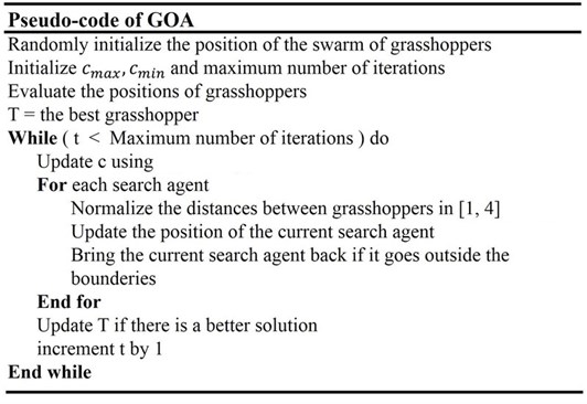
Fig. 4Flowchart of Grasshopper algorithm [20]
![Flowchart of Grasshopper algorithm [20]](https://static-01.extrica.com/articles/22149/22149-img4.jpg)
6. Optimization results
After performing Grasshopper Optimization Algorithm over 500 iterations following optimal results are obtained for surface roughness at the dry, wet and cryogenic cutting conditions as shown in Table 9.
Table 9Optimal parameters obtained from Grasshopper optimization algorithm
Cutting speed () | Feed rate () | Depth of cut (d.o.c.) | Optimal values | |
(Dry) | 160 | 0.3 | 1.01 | 0.3895 |
(Wet) | 200 | 0.3 | 0.5 | 0.4535 |
(Cryogenic) | 165.58 | 0.1 | 1.5 | 0.7916 |
The results obtained from the Grasshopper optimization algorithm are presented in the Fig. 5, 6 and 7 for the dry, wet and cryogenic conditions respectively. As it can be observed that the algorithm solves the problem, and the convergence is obtained in at a very quick level. The total iterations carried were 500 but the convergence obtained is almost around 100 iterations. This shows that the algorithm can solve this complex problem and coming through an optimum result in a quick manner. Here grasshopper optimization algorithm proves its usefulness and applicability in real-life problem.
7. Validation
To validate, the experiment was conducted according to optimal parameters obtained from Grasshopper Optimization Algorithm and the corresponding values for surface roughness were taken as shown in Table 10.
Fig. 5Grasshopper optimization algorithm results for dry condition
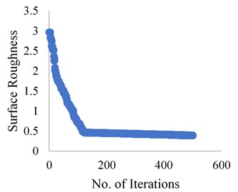
Fig. 6Grasshopper optimization algorithm results for wet condition
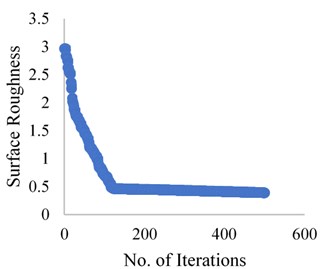
Fig. 7Grasshopper optimization algorithm results for Cryogenic condition
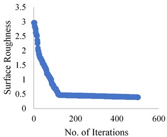
Table 10Comparison between G.O.A. and validated
Optimal values from experimentation | Validated values | Improvement by algorithm % | |
(Dry) | 0.952 | 0.457 | 51.99 |
(Wet) | 0.969 | 0.531 | 45.20 |
(Cryogenic) | 0.803 | 0.801 | 0.24 |
8. Conclusions
The optimal values obtained for surface roughness with the help of the S/N ratio was observed that in the dry condition the influencing factor is feed rate, in the wet condition the influencing factor is the depth of cut and in the cryogenic condition the influencing factor is feed rate. The mathematical modelling is based on Response Surface Methodology which is used to find the relation between output response and several input variables, our objective is to optimize the response variables i.e Surface roughness. It was observed that in the cryogenic condition the values of surface roughness is very less as compared to a dry and wet condition in the set of experiments. Cryogenic machining processing can provide significant improvement in both product quality and productivity. The optimal values for surface roughness are obtained with the help of the Grasshopper Optimization Algorithm using equations obtained from RSM. The validated results show drastic improvement in surface roughness for dry and wet condition improvement observed was 51.99 % and 45.20 % respectively. The values obtained for the cryogenic condition is improved by 0.24 % which is not much of significance.
References
-
I. Ciftci, “Machining of austenitic stainless steels using CVD multi-layer coated cemented carbide tools,” Tribology International, Vol. 39, No. 6, pp. 565–569, Jun. 2006, https://doi.org/10.1016/j.triboint.2005.05.005
-
M. Kaladhar, K. Venkata Subbaiah, C. Srinivasa Rao, and K. Narayana Rao, “Optimization of process parameters in turning of AISI202 austenitic stainless steel,” Journal of Engineering and Applied Sciences, Vol. 5, No. 9, pp. 79–87, Sep. 2010.
-
D. Philip Selvaraj and Chandramohan P., “Optimization of surface roughness of AISI 304 austenitic stainless steel in dry turning operation using Taguchi design method,” Journal of Engineering Science and Technology, Vol. 5, No. 3, Sep. 2010.
-
R. A. Mahdavinejad and S. Saeedy, “Investigation of the influential parameters of machining of AISI 304 stainless steel,” Sadhana, Vol. 36, No. 6, pp. 963–970, Dec. 2011, https://doi.org/10.1007/s12046-011-0055-z
-
Y. Touggui, S. Belhadi, S.-E. Mechraoui, A. Uysal, M. A. Yallese, and M. Temmar, “Multi-objective optimization of turning parameters for targeting surface roughness and maximizing material removal rate in dry turning of AISI 316L with PVD-coated cermet insert,” SN Applied Sciences, Vol. 2, No. 8, Aug. 2020, https://doi.org/10.1007/s42452-020-3167-4
-
T. C. Yap, “Roles of cryogenic cooling in turning of superalloys, ferrous metals, and viscoelastic polymers,” Technologies, Vol. 7, No. 3, p. 63, Sep. 2019, https://doi.org/10.3390/technologies7030063
-
Yasir Muhammad, Ginta Turnad, Ariwahjoedi B., Alkali Adam, and Danish Mohd, “Effect of cutting speed and feed rate on surface roughness of AISI 316l SS using end-milling,” Journal of Engineering and Applied Sciences, Vol. 11, No. 4, pp. 2496–2500, 2016.
-
M. Kaladhar, K. Venkata Subbaiah, and Ch Srinivasa Rao, “Determination of optimum process parameters during turning of AISI 304 austenitic stainless steels using Taguchi method and ANOVA,” International Journal of Lean Thinking, Vol. 3, No. 1, Dec. 2011.
-
D. Umbrello, F. Micari, and I. S. Jawahir, “The effects of cryogenic cooling on surface integrity in hard machining: A comparison with dry machining,” CIRP Annals, Vol. 61, No. 1, pp. 103–106, 2012, https://doi.org/10.1016/j.cirp.2012.03.052
-
S. Katoch, S. S. Chauhan, and V. Kumar, “A review on genetic algorithm: past, present, and future,” Multimedia Tools and Applications, Vol. 80, No. 5, pp. 8091–8126, Feb. 2021, https://doi.org/10.1007/s11042-020-10139-6
-
M. N. K. Kulkarni, M. S. Patekar, M. T. Bhoskar, M. O. Kulkarni, G. M. Kakandikar, and V. M. Nandedkar, “Particle swarm optimization applications to mechanical engineering – a review,” Materials Today: Proceedings, Vol. 2, No. 4-5, pp. 2631–2639, 2015, https://doi.org/10.1016/j.matpr.2015.07.223
-
O. Kulkarni and S. Kulkarni, “Process parameter optimization in WEDM by Grey Wolf optimizer,” Materials Today: Proceedings, Vol. 5, No. 2, pp. 4402–4412, 2018, https://doi.org/10.1016/j.matpr.2017.12.008
-
A. S. Joshi, O. Kulkarni, G. M. Kakandikar, and V. M. Nandedkar, “Cuckoo search optimization – a review,” Materials Today: Proceedings, Vol. 4, No. 8, pp. 7262–7269, 2017, https://doi.org/10.1016/j.matpr.2017.07.055
-
X. S. Yang and X. He, “Bat algorithm: literature review and applications,” International Journal of Bio-Inspired Computation, Vol. 5, No. 3, p. 141, 2013, https://doi.org/10.1504/ijbic.2013.055093
-
S. P. Mhatugade, G. M. Kakandikar, O. K. Kulkarni, and V. M. Nandedkar, “Development of a multi‐objective Salp Swarm Algorithm for Benchmark Functions and Real‐world Problems,” in Optimization for Engineering Problems, Wiley, 2019, pp. 101–130, https://doi.org/10.1002/9781119644552.ch5
-
G. M. Kakandikar, O. Kulkarni, S. Patekar, and T. Bhoskar, “Optimising fracture in automotive tail cap by firefly algorithm,” International Journal of Swarm Intelligence, Vol. 5, No. 1, p. 136, 2020, https://doi.org/10.1504/ijsi.2020.106396
-
Ganesh M. Kakandikar and Vilas M. Nandedkar, Sheet Metal Forming Optimization: Bioinspired Approaches. CRC Press, 2017.
-
O. Kulkarni, N. Kulkarni, A. J. Kulkarni, and G. Kakandikar, “Constrained cohort intelligence using static and dynamic penalty function approach for mechanical components design,” International Journal of Parallel, Emergent and Distributed Systems, Vol. 33, No. 6, pp. 570–588, Nov. 2018, https://doi.org/10.1080/17445760.2016.1242728
-
T. T. Huan, A. J. Kulkarni, J. Kanesan, C. J. Huang, and A. Abraham, “Ideology algorithm: a socio-inspired optimization methodology,” Neural Computing and Applications, Vol. 28, No. S1, pp. 845–876, Dec. 2017, https://doi.org/10.1007/s00521-016-2379-4
-
S. Saremi, S. Mirjalili, and A. Lewis, “Grasshopper optimisation algorithm: Theory and application,” Advances in Engineering Software, Vol. 105, pp. 30–47, Mar. 2017, https://doi.org/10.1016/j.advengsoft.2017.01.004
-
A. G. Neve, G. M. Kakandikar, and O. Kulkarni, “Application of Grasshopper optimization algorithm for constrained and unconstrained test functions,” International Journal of Swarm Intelligence and Evolutionary Computation, Vol. 6, No. 3, 2017, https://doi.org/10.4172/2090-4908.1000165
-
S. S. Wagh, A. P. Kulkarni, and V. G. Sargade, “Machinability studies of austenitic stainless steel (AISI 304) using PVD cathodic arc evaporation (CAE) system deposited AlCrN/TiAlN coated carbide inserts,” Procedia Engineering, Vol. 64, pp. 907–914, 2013, https://doi.org/10.1016/j.proeng.2013.09.167
-
D. V. V. Krishan Prasad Et. Al. (2013), “Influence of cutting parameters on turning process using Anova analysis,” Research Journal of Engineering Sciences, Vol. 2, No. 9, pp. 1–6, 9472.
-
G. M. A. Acayaba and P. M. Escalona, “Prediction of surface roughness in low speed turning of AISI316 austenitic stainless steel,” CIRP Journal of Manufacturing Science and Technology, Vol. 11, pp. 62–67, Nov. 2015, https://doi.org/10.1016/j.cirpj.2015.08.004
-
M. Sarikaya, “Optimization of the surface roughness by applying the Taguchi technique for the turning of stainless steel under cooling conditions,” Materiali in tehnologije, Vol. 49, No. 6, pp. 941–948, Nov. 2015, https://doi.org/10.17222/mit.2014.282
-
Prajwalkumar M. Patil, Rajendrakumar V. Kadi, T. Suresh, Dundur, and Anil S. Pol, “Effect of cutting parameters on surface quality of AISI 316 austenitic stainless steel in CNC turning,” International Research Journal of Engineering and Technology, Vol. 2, No. 4, pp. 1453–1457, Feb. 2018.
-
Rajendra Kumar V. Kadi Et. Al. (2015), “Optimization of dry turning parameters on surface roughness and hardness of Austenitic Stainless steel et.al. (AISI316) by Taguchi Technique,” Journal of Engineering and Fundamentals, Vol. 2, No. 2, pp. 30–41.
About this article

