Two-Stage Performance Engineering of Container-based Virtualization
Two-Stage Performance Engineering of Container-based Virtualization
Volume 3, Issue 1, Page No 521-536, 2018
Author’s Name: Zheng Li1,4, Maria Kihl2,a), Yiqun Chen3, He Zhang1
View Affiliations
1Software Institute, Nanjing University, 210008, China
2Department of Electrical and Information Technology, Lund University, 223 63, Sweden
3Centre for Spatial Data Infrastructures & Land Administration, University of Melbourne, 3010, Australia
4Department of Computer Science, University of Concepci´on, 4070386, Chile
a)Author to whom correspondence should be addressed. E-mail: maria.kihl@eit.lth.se
Adv. Sci. Technol. Eng. Syst. J. 3(1), 521-536 (2018); ![]() DOI: 10.25046/aj030163
DOI: 10.25046/aj030163
Keywords: Cloud Computing, Container, Hypervisor, MapReduce, Performance Engineering, Virtualization

Export Citations
Cloud computing has become a compelling paradigm built on compute and storage virtualization technologies. The current virtualization solution in the Cloud widely relies on hypervisor-based technologies. Given the recent booming of the container ecosystem, the container-based virtualization starts receiving more attention for being a promising alternative. Although the container technologies are generally considered to be lightweight, no virtualization solution is ideally resource-free, and the corresponding performance overheads will lead to negative impacts on the quality of Cloud services. To facilitate understanding container technologies from the performance engineering’s perspective, we conducted two-stage performance investigations into Docker containers as a concrete example. At the first stage, we used a physical machine with “just-enough” resource as a baseline to investigate the performance overhead of a standalone Docker container against a standalone virtual machine (VM). With findings contrary to the related work, our evaluation results show that the virtualization’s performance overhead could vary not only on a feature-by-feature basis but also on a job-to-job basis. Moreover, the hypervisor-based technology does not come with higher performance overhead in every case. For example, Docker containers particularly exhibit lower QoS in terms of storage transaction speed. At the ongoing second stage, we employed a physical machine with “fair-enough” resource to implement a container-based MapReduce application and try to optimize its performance. In fact, this machine failed in affording VM-based MapReduce clusters in the same scale. The performance tuning results show that the effects of different optimization strategies could largely be related to the data characteristics. For example, LZO compression can bring the most significant performance improvement when dealing with text data in our case.
Received: 14 November 2017, Accepted: 05 February 2018, Published Online: 28 February 2018
Introduction
IEEE International Conference on Advanced Information Networking and Application (AINA 2017) [1].
The container technologies have widely been accepted The Cloud has been considered to be able to profor building next-generation Cloud systems. This pa- vide computing capacity as the next utility in our modper investigates the performance overhead of container- ern daily life. In particular, it is the virtualization based virtualization and the performance optimization technologies that enable Cloud computing to be a new of a container-based MapReduce application, which is paradigm of utility, by playing various vital roles in an extension of work originally presented in the 31st supporting Cloud services, ranging from resource iso-
lation to resource provisioning. The existing virtualization technologies can roughly be distinguished between the hypervisor-based and the container-based solutions. Considering their own resource consumption, both virtualization solutions inevitably introduce performance overheads to running Cloud services, and the performance overheads could then lead to negative impacts to the corresponding quality of service (QoS). Therefore, it would be crucial for both Cloud providers (e.g., for improving infrastructural efficiency) and consumers (e.g., for selecting services wisely) to understand to what extend a candidate virtualization solution incurs influence on the Cloud’s QoS.
Recall that hypervisor-driven virtual machines (VMs) require guest operating systems (OS), while containers can share a host OS. Suppose physical machines, VMs and containers are three candidate resource types for a particular Cloud service, a natural hypothesis could be:
The physical machine-based service has the best quality among the three resource types, while the container-based service performs better than the hypervisor-based VM service.
Unfortunately, to the best of our knowledge, there is little quantitative evidence to help test this hypothesis in an “apple-to-apple” manner, except for the similar qualitative discussions. Furthermore, the performance overhead of hypervisor-based and containerbased virtualization technologies can even vary in practice depending on different service circumstance (e.g., uncertain workload densities and resource competitions). Therefore, we decided to conduct a twofold investigation into containers from the performance’s perspective. Firstly, we used a physical machine with “just-enough” resource as a baseline to quantitatively investigate and compare the performance overheads between the container-based and hypervisor-based virtualizations. In particular, since Docker is currently the most popular container solution [2] and VMWare is one of the leaders in the hypervisor market [3], we chose Docker and VMWare Workstation 12 Pro to represent the two virtualization solutions respectively. Secondly, we implemented a container-based MapReduce cluster on a physical machine with “fair-enough” resource to investigate the performance optimization of our MapReduce application at least in this use case.
According to the clarifications in [4, 5], our qualitative investigations can be regulated by the discipline of experimental computer science (ECS). By employing ECS’s recently available Domain Knowledge-driven Methodology (DoKnowMe) [6], we experimentally explored the performance overheads of different virtualization solutions on a feature-by-feature basis, i.e. the communication-, computation-, memory- and storagerelated QoS aspects. As for the investigation into performance optimization, we were concerned with the task timeout, out-of-band heartbeat, buffer setting, stream merging, data compression and the cluster size of our container-based MapReduce application.
The experimental results and analyses of performance overhead investigation generally advocate the aforementioned hypothesis. However, the hypothesis is not true in all the cases. For example, we do not see computation performance difference between the three resource types for solving a combinatorially hard chess problem; and the container exhibits even higher storage performance overhead than the VM when reading/writing data byte by byte. Moreover, we find that the remarkable performance loss incurred by both virtualization solutions usually appears in the performance variability.
The performance optimization investigation reveals that various optimization strategies might take different effects due to different data characteristics of a container-based MapReduce application. For example, dealing with text data can significantly benefit from enabling data compression, whereas buffer settings have little effect for dealing with relatively small amount of data.
Overall, our work makes fourfold contributions to the container ecosystem, as specified below.
(1) Our experimental results and analyses can help both researchers and practitioners to better understand the fundamental performance of the present container-based and hypervisor-based virtualization technologies. In fact, the performance evaluation practices in ECS can roughly be distinguished between two stages: the first stage is to reveal the primary performance of specific (system) features, while the second stage is generally based on the first-stage evaluation to investigate real-world application cases. Thus, this work can be viewed as a foundation for more sophisticated evaluation studies in the future.
(2) Our method of calculating performance overhead can easily be applied or adapted to different evaluation scenarios by others. The literature shows that the “performance overhead” has normally been used in the context of qualitative discussions. By quantifying such an indicator, our study essentially provides a concrete lens into the case of performance comparisons.
(3) As a second-stage evaluation work, our case study on the performance optimization of a MapReduce application both demonstrates a practical use case and supplies an easy-toreplicate scenario for engineering performance of container-based applications. In other words, this work essentially proposed a characteristicconsistent data set (i.e. Amazon’s spot price history that is open to the public) for future performance engineering studies.
(4) The whole evaluation logic and details reported in this paper can be viewed as a reusable template of evaluating Docker containers. Since the Docker project is still quickly growing [7], the evaluation results could be gradually out of date. Given this template, future evaluations
can be conveniently repeated or replicated even by different evaluators at different times and locations. More importantly, by emphasizing the backend logic and evaluation activities, the template-driven evaluation implementations (instead of results only) would be more traceable and comparable.
The remainder of this paper is organized as follows. Section 2 briefly summarizes the background knowledge of container-based and the hypervisor-based virtualization technologies. Section 3 introduces the fundamental performance evaluation of a single container. The detailed performance overhead investigation is divided into two reporting parts, namely pre-experimental activities and experimental results & analyses, and they are correspondingly described into Section 3.2 and 3.3 respectively. Section 4 explains our case study on the performance optimization of a container-based MapReduce application. Section 5 highlights the existing work related to container’s performance evaluation. Conclusions and some future work are discussed in Section 6.
2 Hypervisor-based vs. Containerbased Virtualization
When it comes to the Cloud virtualization, the de facto solution is to employ the hypervisor-based technologies, and the most representative Cloud service type is offering VMs [8]. In this virtualization solution, the hypervisor manages physical computing resources and makes isolated slices of hardware available for creating VMs [7]. We can further distinguish between two types of hypervisors, namely the bare-metal hypervisor that is installed directly onto the computing hardware, and the hosted hypervisor that requires a host OS. To make a better contrast between the hypervisor-related and container-related concepts, we particularly emphasize the second hypervisor type, as shown in Figure 1a. Since the hypervisor-based virtualization provides access to physical hardware only, each VM needs a complete implementation of a guest OS including the binaries and libraries necessary for applications [9]. As a result, the guest OS will inevitably incur resource competition against the applications running on the VM service, and essentially downgrade the QoS from the application’s perspective. Moreover, the performance overhead of the hypervisor would also be passed on to the corresponding Cloud services and lead to negative impacts on the QoS.
To relieve the performance overhead of hypervisorbased virtualization, researchers and practitioners recently started promoting an alternative and lightweight solution, namely container-based virtualization. In fact, the foundation of the container technology can be traced back to the Unix chroot command in 1979 [9], while this technology is eventually evolved into virtualization mechanisms like Linux VServer, OpenVZ and Linux Containers (LXC) along with the booming of Linux [10]. Unlike the hardware-level solution of hypervisors, containers realize virtualization at the OS level and utilize isolated slices of the host OS to shield their contained applications [9]. In essence, a container is composed of one or more lightweight images, and each image is a prebaked and replaceable file system that includes necessary binaries, libraries or middlewares for running the application. In the case of multiple images, the read-only supporting file systems are stacked on top of each other to cater for the writable top-layer file system [2]. With this mechanism, as shown in Figure 1b, containers enable applications to share the same OS and even binaries/libraries when appropriate. As such, compared to VMs, containers would be more resource efficient by excluding the execution of hypervisor and guest OS, and more time efficient by avoiding booting (and shutting down) a whole OS [11, 7]. Nevertheless, it has been identified that the cascading layers of container images come with inherent complexity and performance penalty [12]. In other words, the container-based virtualization technology could also negatively impact the corresponding QoS due to its performance overhead.
 Figure 1: Different architectures of hypervisor-based and container-based virtual services.
3 Fundamental Performance Evaluation of a Single Container
3.1 Performance Evaluation Methodology
Since the comparison between the container’s and the VM’s performance overheads is essentially based on their performance evaluation, we define our work as a performance evaluation study that belongs to the field of experimental computer science [4, 5]. Considering that “evaluation methodology underpins all innovation in experimental computer science” [13], we employ the methodology DoKnowMe [6] to guide evaluation implementations in this study. DoKnowMe is an abstract evaluation methodology on the analogy of “class” in object-oriented programming. By integrating domain-specific knowledge artefacts, DoKnowMe can be customized into specific methodologies (by analogy of “object”) to facilitate evaluating different concrete computing systems. The skeleton of DoKnowMe is composed of ten generic evaluation steps, as listed below.
(1) Requirement recognition;
(2) Service feature identification;
(3) Metrics and benchmarks listing;
(4) Metrics and benchmarks selection;
(5) Experimental factors listing;
(6) Experimental factors selection;
(7) Experiment design;
(8) Experiment implementation;
(9) Experimental analysis;
(10) Conclusion and documentation.
Each evaluation step further comprises a set of activities together with the corresponding evaluation strategies. The elaboration on these evaluation steps is out of the scope of this paper. To better structure our report, we divide the evaluation implementation into pre-experimental activities and experimental results & analyses.
3.2 Pre-Experimental Activities
3.2.1 Requirement Recognition
Following DoKnowMe, the whole evaluation implementation is essentially driven by the recognized requirements. In general, the requirement recognition is to define a set of specific requirement questions both to facilitate understanding the real-world problem and to help achieve clear statements of the corresponding evaluation purpose. In this case, the basic requirement is to give a fundamental quantitative comparison between the hypervisor-based and container-based virtualization solutions. As mentioned previously, we concretize these two virtualization solutions into VMWare Workstation VMs and Docker containers respectively, in order to facilitate our evaluation implementation (i.e., using a physical machine as a baseline to investigate the performance overhead of a Docker container against a VM). Thus, such a requirement can further be specified into two questions:
RQ1: How much performance overhead does a standalone Docker container introduce over its base physical machine?
RQ2: How much performance overhead does a standalone VM introduce over its base physical machine?
Considering that virtualization technologies could lead to variation in the performance of Cloud services [14], we are also concerned with the container’s and VM’s potential variability overhead besides their average performance overhead:
RQ3: How much performance variability overhead does a standalone Docker container introduce over its base physical machine during a particular period of time?
RQ4: How much performance variability overhead does a standalone VM introduce over its base physical machine during a particular period of time?
3.2.2 Service Feature Identification
Recall that we treat Docker containers as an alternative type of Cloud service to VMs. By using the taxonomy of Cloud services evaluation [15], we directly list the service feature candidates, as shown in Figure 2. Note that a service feature is defined as a combination of a physical property and its capacity, and we individually examine the four physical properties in this study:
- Communication
- Computation
- Memory
- Storage
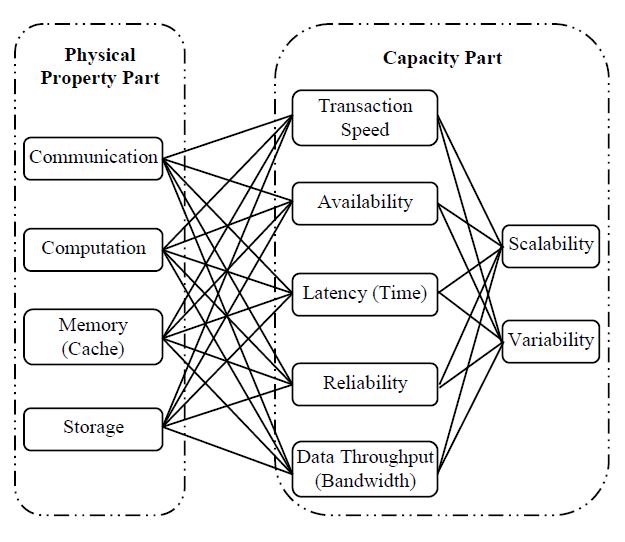 Figure 2: Candidate service features for evaluating Cloud service performance (cf. [15]).
3.2.3 Metrics/Benchmarks Listing and Selection
The selection of evaluation metrics usually depends on the availability of benchmarks. According to our previous experience of Cloud services evaluation, we choose relatively lightweight and popular benchmarks to try to minimize the benchmarking overhead, as listed in Table 1. For example, Iperf has been identified to be able to deliver more precise results by consuming less system resources. In fact, except for STREAM that is the de facto memory evaluation benchmark included in the HPC Challenge Benchmark (HPCC) suite, the other benchmarks are all Ubuntu’s built-in utilities.
Table 1: Metrics and benchmarks for this evaluation study.
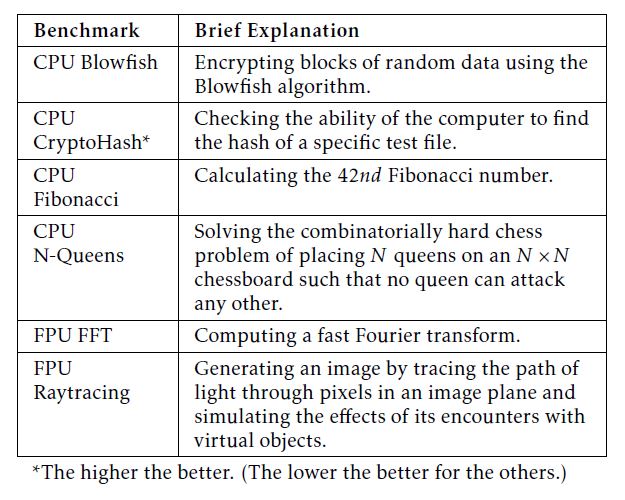
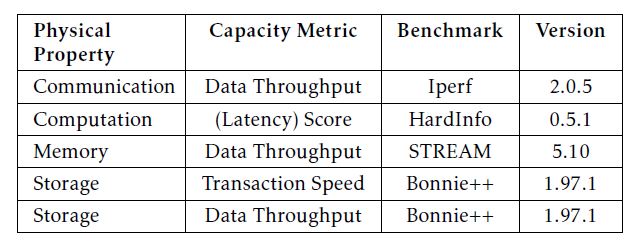 In particular, although Bonnie++ only measures the amount of data processed per second, the disk I/O transactions are on a byte-by-byte basis when accessing small size of data. Therefore, we consider to measure storage transaction speed when operating byte-size data and measure storage data throughput when operating block-size data. As for the property computation, considering the diversity in CPU jobs (e.g., integer and floating-point calculations), we employ HardInfo that includes six micro-benchmarks to generate performance scores, as briefly explained in Table 2. HardInfo is a tool package that can summarize the information about the host machine’s hardware and operating system, as well as benchmarking the CPU. In this study, we employ HardInfo for CPU benchmarking only.
Table 2: Micro-benchmarks included in HardInfo.
 When it comes to the performance overhead, we use the business domain’s Overhead Ratio as an analogy to its measurement. In detail, we treat the performance loss compared to a baseline as the expense, while imagining the baseline performance to be the overall income, as defined in Equation (1).
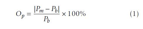
where Op refers to the performance overhead; Pm denotes the benchmarking result as a measurement of a service feature; Pb indicates the baseline performance of the service feature; and then |Pm − Pb| represents the corresponding performance loss. Note that the physical machine’s performance is used as the baseline in our study. Moreover, considering possible observational errors, we allow a margin of error for the confidence level as high as 99% with regarding to the benchmarking results. In other words, we will ignore the difference between the measured performance and its baseline if the calculated performance overhead is less than 1% (i.e. if Op < 1%, then Pm = Pb).
3.2.4 Experimental Factor Listing and Selection
The identification of experimental factors plays a prerequisite role in the following experimental design. More importantly, specifying the relevant factors would be necessary for improving the repeatability of experimental implementations. By referring to the experimental factor framework of Cloud services evaluation [16], we choose the resource- and workloadrelated factors as follows.
The resource-related factors:
- Resource Type: Given the evaluation requirement, we have essentially considered three types of resources to support the imaginary Cloud service, namely physical machine, container and VM.
- Communication Scope: We test the communication between our local machine and an Amazon EC2 t2.micro instance. The local machine is located in our broadband lab at Lund University, and the EC2 instance is from Amazon’s available zone ap-southeast-1a within the region Asia Pacific (Singapore).
- Communication Ethernet Index: Our local side uses a Gigabit connection to the Internet, while the EC2 instance at remote side has the “Low to Moderate” networking performance defined by Amazon.
- CPU Index: The physical machine’s CPU model is Intel Core™2 Duo Processor T7500. The processor has two cores with the 64-bit architecture, and its base frequency is 2.2 GHz. We allocate both CPU cores to the standalone VM upon the physical machine.
- Memory Size: The physical machine is equipped with a 3GB DDR2 SDRAM. When running the
VMWare Workstation Pro without launching any VM, “watch -n 5 free -m” shows a memory usage of 817MB while leaving 2183MB free in the physical machine. Therefore, we set the memory size to 2GB for the VM to avoid (at least to minimize) the possible memory swapping.
- Storage Size: There are 120GB of hard disk in the physical machine. Considering the space usage by the host operating system, we allocate 100GB to the VM.
- Operating System: Since Docker requires a 64bit installation and Linux kernels older than
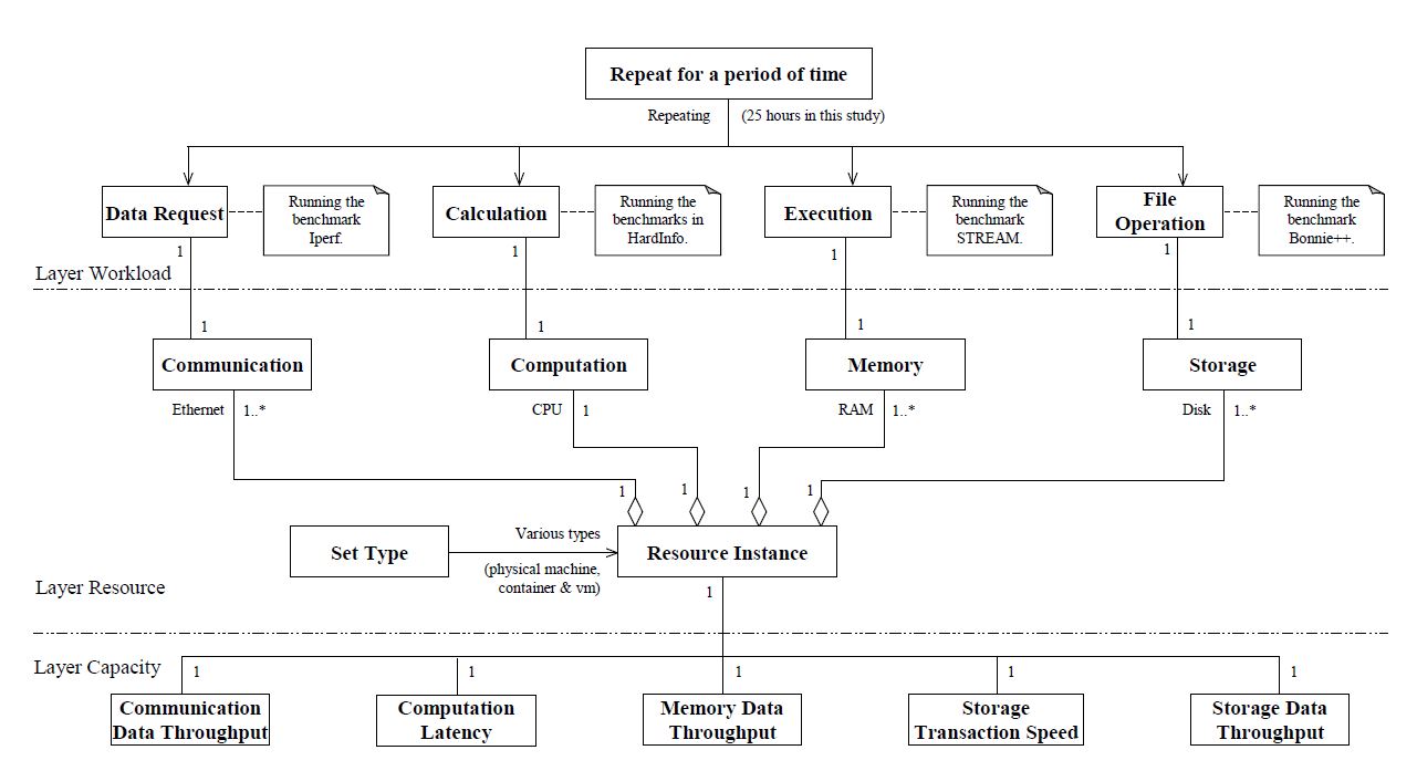 Figure 3: Experimental blueprint for evaluating three types of resources in this study.
3.10 do not support all the features for running Docker containers, we choose the latest 64bit Ubuntu 15.10 as the operating system for both the physical machine and the VM. In addition, according to the discussions about base images in the Docker community [17, 18], we intentionally set an OS base image (by specifying FROM ubuntu:15.10 in the Dockerfile) for all the Docker containers in our experiments. Note that a container’s OS base image is only a file system representation, while not acting as a guest OS.
The workload-related factors:
- Duration: For each evaluation experiment, we decided to take a whole-day observation plus one-hour warming up (i.e. 25 hours).
- Workload Size: The experimental workloads are predefined by the selected benchmarks. For example, the micro-benchmark CPU Fibonacci generates workload by calculating the 42nd Fibonacci number (cf. Table 2). In particular, the benchmark Bonnie++ distinguishes between reading/writing byte-size and block-size data.
3.2.5 Experimental Design
It is clear that the identified factors are all with single value except for the Resource Type. Therefore, a straightforward design is to run the individual benchmarks on each of the three types of resources independently for a whole day plus one hour.
Furthermore, following the conceptual model of IaaS performance evaluation [19], we record the experimental design into a blueprint both to facilitate our experimental implementations and to help other evaluators replicate/repeat our study. In particular, the experimental elements are divided into three layers
(namely Layer Workload, Layer Resource, and Layer Capacity), as shown in Figure 3. To avoid duplication, we do not elaborate the detailed elements in this blueprint.
3.3 Experimental Results and Analyses
3.3.1 Communication Evaluation Result and Analysis
Docker creates a virtual bridge docker0 on the host machine to enable both the host-container and the container-container communications. In particular, it is the Network Address Translation (NAT) that forwards containers’ traffic to external networks. For the purpose of “apple-to-apple” comparison, we also configure VM’s network type as NAT that uses the VMnet8 virtual switch created by VMware Workstation.
Using NAT, both Docker containers and VMs can establish outgoing connections by default, while they require port binding/forwarding to accept incoming connections. To reduce the possibility of configurational noise, we only test the outgoing communication performance, by setting the remote EC2 instance to Iperf server and using the local machine, container and VM all as Iperf clients.
The benchmarking results of repeating iperf -c XXX.XXX.XXX.XXX -t 15 (with a one-minute interval between every two consecutive trials) are listed in Table 3. The XXX.XXX.XXX.XXX denotes the external IP address of the EC2 instance used in our experiments. Note that, unlike the other performance features, the communication data throughput delivers periodical and significant fluctuations, which might be a result from the network resource competition at both our local side and the EC2 side during working hours. Therefore, we particularly focus on the longest period of relatively stable data out of the whole-day observation, and thus the results here are for rough reference only.
Table 3: Communication benchmarking results using Iperf.
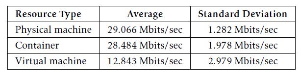 Given the extra cost of using the NAT network to send and receive packets, there would be unavoidable performance penalties for both the container and the VM. Using Equation (1), we calculate their communication performance overheads, as illustrated in Figure 4.
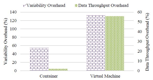 Figure 4: Communication data throughput and its variability overhead of a standalone Docker container vs. VM (using the benchmark Iperf).
A clear trend is that, compared to the VM, the container loses less communication performance, with only 2% data throughput overhead and around 54% variability overhead. However, it is surprising to see a more than 55% data throughput overhead for the VM. Although we have double checked the relevant configuration parameters and redone several rounds of experiments to confirm this phenomenon, we still doubt about the hypervisor-related reason behind such a big performance loss. We particularly highlight this observation to inspire further investigations.
3.3.2 Computation Evaluation Result and Analysis
Recall that HardInfo’s six micro benchmarks deliver both “higher=better” and “lower=better” CPU scores (cf. Table 2). To facilitate experimental analysis, we use the two equations below to standardize the “higher=better” and “lower=better” benchmarking results respectively.
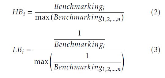 where HBi further scores the service resource type i by standardizing the “higher=better” benchmarking result Benchmarkingi; and similarly, LBi represents the standardized “lower=better” CPU score of the service resource type i. Note that Equation (3) essentially offers the “lower=better” benchmarking results a “higher=better” representation through reciprocal standardization.
For the purpose of conciseness, here we only specify the standardized experimental results, as shown in Table 4. Exceptionally, the container and VM have slightly higher CPU N-Queens scores than the physical machine. Given the predefined observational margin of error (cf. Section 3.2.3), we are not concerned with this trivial difference, while treating their performance values as equal to each other in this case.
Table 4: Standardized computation benchmarking results using HardInfo.
We can further use a radar plot to help ignore the trivial number differences, and also help intuitively contrast the performance of the three resource types, as demonstrated in Figure 5. For example, the different polygon sizes clearly indicate that the container generally computes faster than the VM, although the performance differences are on a case-by-case basis with respect to different CPU job types.
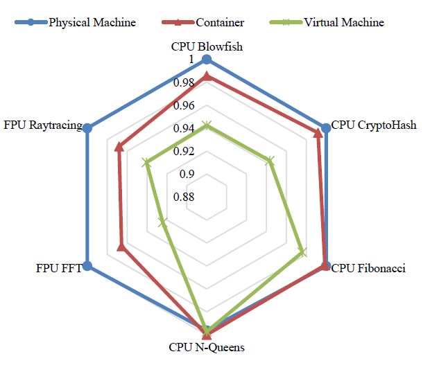 Figure 5: Computation benchmarking results by using HardInfo.
Nevertheless, our experimental results do not display any general trend in variability of those resources’ computation scores. As can be seen from the calculated performance overheads (cf. Figure 6), the VM does not even show worse variability than the physical machine when running CPU CryptoHash, CPU N-Queens and FPU Raytracing. On the contrary, there is an almost 2500% variability overhead for the VM when calculating the 42nd Fibonacci number. In particular, the virtualization technologies seem to be sensitive to the Fourier transform jobs (the benchmark FPU FFT), because the computation latency overhead and the variability overhead are relatively high for both the container and the VM.
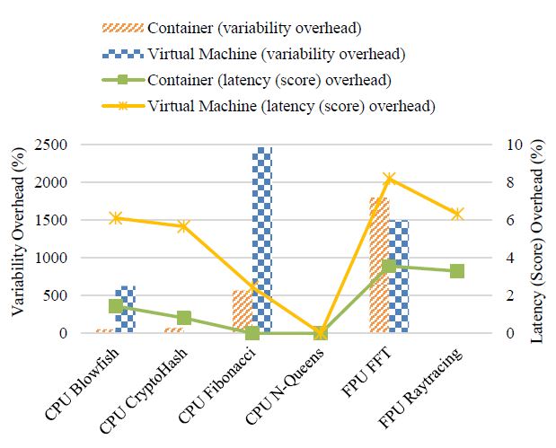 Figure 6: Computation latency (score) and its variability overhead of a standalone Docker container vs. VM (using the tool kit HardInfo).
3.3.3 Memory Evaluation Result and Analysis
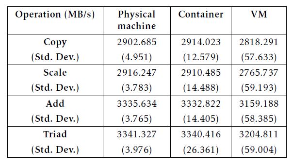
STREAM measures sustainable memory data throughput by conducting four typical vector operations, namely Copy, Scale, Add and Triad. The memory benchmarking results are listed in Table 5. We further visualize the results into Figure 7 to facilitate our observation. As the first impression, it seems that the VM has a bit poorer memory data throughput, and there is little difference between the physical machine and the Docker container in the context of running STREAM.
Table 5: Memory benchmarking results using STREAM.
 By calculating the performance overhead in terms of memory data throughput and its variability, we are able to see the significant difference among these three types of resources, as illustrated in Figure 8. Take the operation Triad as an example, although the container performs as well as the physical machine on average, the variability overhead of the container is more than 500%; similarly, although the VM’s Triad data throughput overhead is around 4% only, its variability overhead is almost 1400%. In other words, the memory performance loss incurred by both virtualization techniques is mainly embodied with the increase in the performance variability.
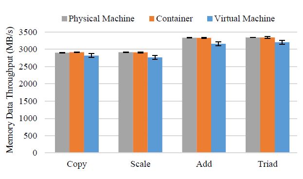 Figure 7: Memory benchmarking results by using STREAM. Error bars indicate the standard deviations of the corresponding memory data throughput.
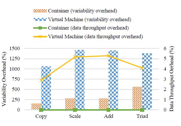 Figure 8: Memory data throughput and its variability overhead of a standalone Docker container vs. VM (using the benchmark STREAM).
In addition, it is also worth notable that the container’s average Copy data throughput is even slightly higher than the physical machine (i.e. 2914.023MB/s vs. 2902.685MB/s) in our experiments. Recall that we have considered a 1% margin of error. Since those two values are close to each other within this error margin, here we ignore such an irregular phenomenon as an observational error.
3.3.4 Storage Evaluation Result and Analysis
For the test of disk reading and writing, Bonnie++ creates a dataset twice the size of the involved RAM memory. Since the VM is allocated 2GB of RAM, we also restrict the memory usage to 2GB for Bonnie++ on both the physical machine and the container, by running “sudo bonnie++ -r 2048 -n 128 -d / -u root”. Correspondingly, the benchmarking trials are conducted with 4GB of random data on the disk. When Bonnie++ is running, it carries out various storage operations ranging from data reading/writing to file creating/deleting. Here we only focus on the performance of reading/writing byte- and block-size data.
To help highlight several different observations, we plot the trajectory of the experimental results along the trial sequence during the whole day, as shown in Figure 9. The first surprising observation is that, all the three resource types have regular patterns of performance jitter in block writing, rewriting and reading. Due to the space limit, we do not report their block rewriting performance in this paper. By exploring the hardware information, we identified the hard disk drive (HDD) model to be ATA Hitachi HTS54161, and its specification describes “It stores 512 bytes per sector and uses four data heads to read the data from two platters, rotating at 5,400 revolutions per minute”. As we know, the hard disk surface is divided into a set of concentrically circular tracks. Given the same rotational speed of an HDD, the outer tracks would have higher data throughput than the inner ones. As such, those regular patterns might indicate that the HDD heads sequentially shuttle between outer and inner tracks when consecutively writing/reading block data during the experiments.
The second surprising observation is that, unlike most cases in which the VM has the worst performance, the container seems significantly poor at accessing the byte size of data, although its performance variability is clearly the smallest. We further calculate the storage performance overhead to deliver more specific comparison between the container and the VM, and draw the results into Figure 10. Note that, in the case when the container’s/VM’s variability is smaller than the physical machine’s, we directly set the corresponding variability overhead to zero rather than allowing any performance overhead to be negative. Then, the bars in the chart indicate that the storage variability overheads of both virtualization technologies are nearly negligible except for reading byte-size data on the VM (up to nearly 200%). The lines show that the container brings around 40% to 50% data throughput overhead when performing disk operations on a byte-by-byte basis. On the contrary, there is relatively trivial performance loss in VM’s byte data writing. However, the VM has roughly 30% data throughput overhead in other disk I/O scenarios, whereas the container barely incurs overhead when reading/writing large size of data.
Our third observation is that, the storage performance overhead of different virtualization technologies can also be reflected through the total number of the iterative Bonnie++ trials. As pointed by the maximum x-axis scale in Figure 9, the physical machine, the container and the VM can respectively finish 150, 147 and 101 rounds of disk tests during 24 hours. Given this information, we estimate the container’s and the VM’s storage performance overhead to be 2% (= |147−150|/150) and 32.67% (= |101−150|/150) respectively.
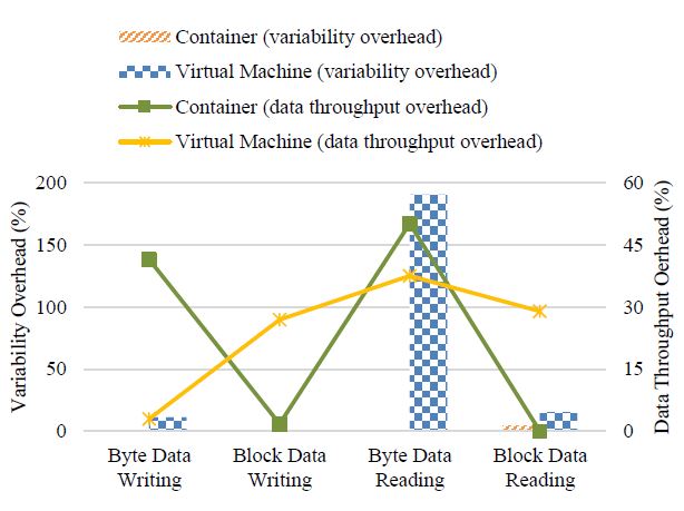 Figure 10: Storage data throughput and its variability overhead of a standalone Docker container vs. VM (using the benchmark Bonnie++).
3.4 Performance Evaluation Conclusion
Following the performance evaluation methodology DoKnowMe, we draw conclusions mainly by answering the predefined requirement questions. Driven by RQ1 and RQ2, our evaluation result largely confirms the aforementioned qualitative discussions: The container’s average performance is generally better than the VM’s and is even comparable to that of the physical machine with regarding to many features. Specifically, the container has less than 4% performance overhead in terms of communication data throughput, computation latency, memory data throughput and storage data throughput. Nevertheless, the container-based virtualization could hit a bottleneck of storage transaction speed, with the overhead up to 50%. Note that, as mentioned previously, we interpret the byte-size data throughput into storage transaction speed, because each byte essentially calls a disk transaction here. In contrast, although the VM delivers the worst performance in most cases, it could perform as well as the physical machine when solving the N-Queens problem or writing small-size data to the disk. By further comparing the storage filesystems of those two types of virtualization technologies, we believe that it is the copy-on-write mechanism that makes containers poor at storage transaction speed.
Driven by RQ3 and RQ4, we find that the performance loss resulting from virtualizations is more visible in the performance variability. For example, the container’s variability overhead could reach as high as over 500% with respect to the Fibonacci calculation and the memory Triad operation. Similarly, although the container generally shows less performance variability than the VM, there are still exceptional cases: The container has the largest performance variation in the job of computing Fourier transform, whereas even the VM’s performance variability is not worse than the physical machine’s when running CryptoHash, NQueens, and Raytracing jobs.
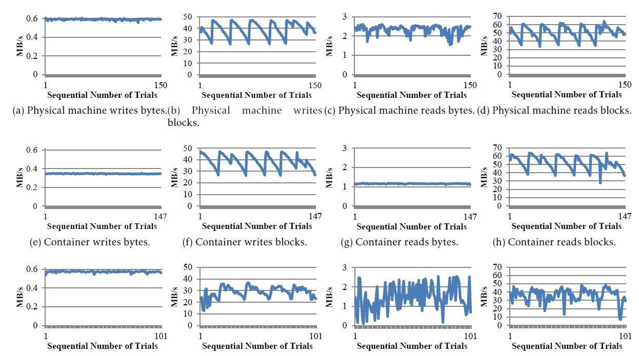 Figure 9: Storage benchmarking results by using Bonnie++ during 24 hours. The maximum x-axis scale indicates the iteration number of the Bonnie++ test (i.e. the physical machine, the container and the VM run 150, 147 and 101 tests respectively).
4 Container-based Application Case Study and Performance Optimization
4.1 Motive from a Background Project
Adequate pricing techniques play a key role in successful Cloud computing [20]. In the de facto Cloud market, there are generally three typical pricing schemes, namely on-demand pricing scheme, reserved pricing scheme, and spot pricing scheme. Although the fixed pricing schemes are dominant approaches to trading Cloud resources nowadays, spot pricing has been broadly agreed as a significant supplement for building a full-fledged market economy for the Cloud ecosystem [21]. Similar to the dynamic pricing in the electricity distribution industry, the spot pricing scheme here also employs a market-driven mechanism to provide spot service at a reduced and fluctuating price, in order to attract more demands and better utilize idle compute resources [22].
Unfortunately, the backend details behind changing spot prices are invisible for most of the Cloud market participants. In fact, unlike the static and straightforward pricing schemes of on-demand and reserved Cloud services, the market-driven mechanism for pricing Cloud spot service has been identified to be complicated both for providers to implement and for consumers to understand.
Therefore, it has become popular and valuable to take Amazon’s spot service as a practical example to investigate Cloud spot pricing, so as to encourage and facilitate more players to enter the Cloud spot market. We are currently involved in a project on Cloud spot pricing analytics by using the whole-year price history of Amazon’s 1053 types of spot service instances. Since Amazon only offers the most recent 60-day price trace to the public for review, we downloaded the price traces monthly in the past year to make sure the completeness of the whole-year price history.
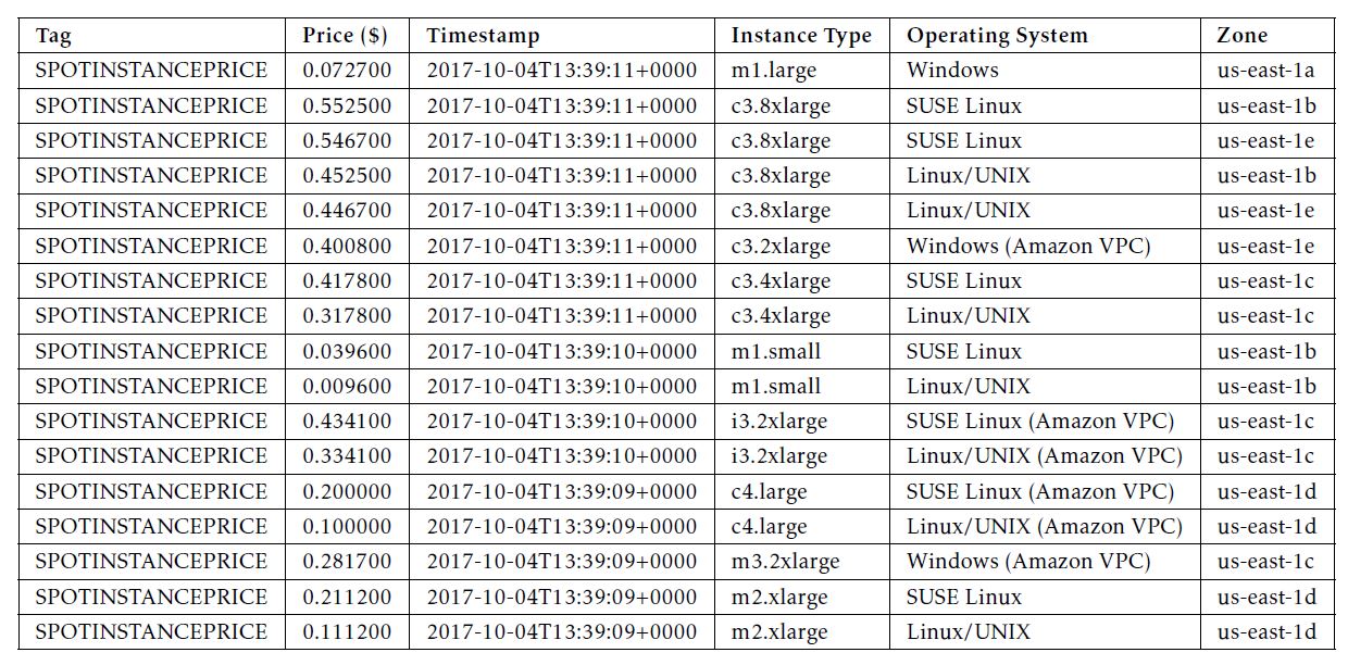
In this way of downloading price traces, it is clear that around half of the overall raw data are duplicate. Moreover, the original price trace is sorted by the timestamp only, as shown in Table 6. To analyze spot service pricing on an instance-by-instance basis, however, the collected price data need not only to be sorted by timestamp but also to be distinguished by the other three attributes, i.e. Instance Type, Operating System and Zone. Thus, we decided to implement a preprocessing program to help clean the data, including removing the duplicate price records and categorizing price traces for individual service instances.
Table 6: A small piece of Amazon’s spot price trace.
 4.2 WordCount-alike Solution
Given the aforementioned requirement of data cleaning, we propose a WordCount-alike solution by analogy. WordCount is a well-known application that calculates the numbers of occurrences of different words within a document or word set. In the domain of big data analytics, WordCount is now a classic application to demonstrate the MapReduce mechanism that has become a standard programming model since 2004 [23]. As shown in Figure 11, the key steps in a MapReduce workflow are:
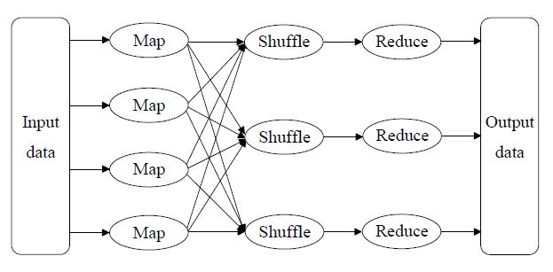 Figure 11: Workflow of the MapReduce process.
(1) The initial input source data are segmented into blocks according to the predefined split function and saved as a list of key-value pairs.
(2) The mapper executes the user-defined map function which generates intermediate key-value pairs.
(3) The intermediate key-value pairs generated by mapper nodes is sent to a specific reducer based on the key.
(4) Each reducer computes and reduces the data to one single key-value pair.
(5) All the reduced data are integrated into the final result of a MapReduce job.
Benefiting from MapReduce, applications like WordCount can deal with large amounts of data parallelly and distributedly. For the purpose of conciseness, we use a three-file scenario to demonstrate the process of MapReduce-based WordCount, as illustrated in Figure 12. In brief, the input files are broken into a set of <key, value> pairs for individual words, then the <key, value> pairs are shuffled alphabetically to facilitate summing up the values (i.e. the occurrence counts) for each unique key, and the reduced results are also a set of <key, value> pairs that directly act as the output in this case.
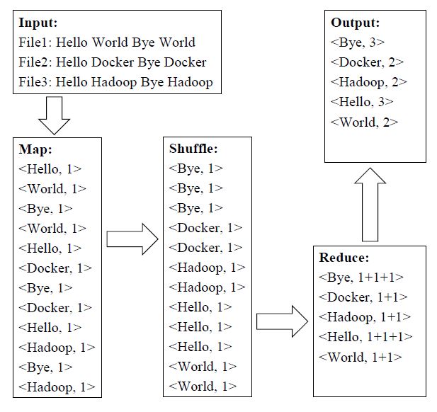 Figure 12: A Three-file Scenario of MapReduce-based WordCount.
Recall that the information of Amazon’s spot price trace is composed of Tag, Price, Timestamp, Instance Type and Zone (cf. Table 6). By considering the value in each information field to be a letter, we treat every single spot price record as an English word. For example, by random analogy, the spot price record “tag price1 time1 OS1 zone1” can be viewed as a six-letter word like “Hadoop”, as highlighted in Figure 13.
As such, we are able to follow the logic of WordCount to fulfill the needs of cleaning our collected spot price history. In particular, instead of summing up the occurrences of the same price records, the duplicate records are simply ignored (removed). Moreover, the price records are sorted by the order of values of Instance Type, Operating System, Zone and Timestamp sequentially during the shuffling stage, while Tag and Price are not involved in data sorting. To avoid duplication, here we do not further elaborate the MapReducebased data cleaning process.
4.3 Application Environment and Implementation
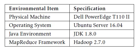
Unlike using “just-enough” environment for microlevel performance evaluation, here we employ “fair-enough” hardware resource to implement the MapReduce-based WordCount application, as listed in Table 7. In detail, the physical machine is Dell PowerEdge T110 II with the CPU model Intel Xeon E3-1200 series E3-1220 / 3.1 GHz. When preparing the MapReduce framework, we choose Apache Hadoop 2.7.0 [24] running in the operating system Ubuntu Server 16.04, and using Docker containers to construct a Hadoop cluster. In particular, Docker allows us to create an exclusive bridge network for the Hadoop cluster by using a specific name, e.g., sudo docker network create –driver=bridge cluster.
Table 7: Summary of application environment.
 In our initial implementation, we realized a threenode Hadoop cluster by packing Hadoop 2.7.0 into a Docker image and starting one master container and two slave ones. As illustrated in Figure 14, such a Hadoop cluster can logically be divided into a disning a MapReduce application, the main interactions are:
HDFS layer
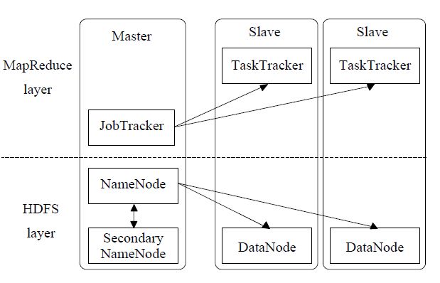 Figure 14: A three-node Hadoop cluster.
(1) A MapReduce job can run in a Hadoop cluster.
(2) The JobTracker in the cluster accepts a job from the MapReduce application, and locates relevant data through the NameNode.
(3) Suitable TaskTrackers are selected and then accept the tasks delivered by the JobTracker.
(4) The JobTracker communicates with the TaskTrackers and manages failures.
(5) When the collaboration among the TaskTrackers finish the job, the JobTracker updates its status and returns the result.
4.4 Performance Optimization Strategies
It is known that the performance of MapReduce applications can be tuned by adjusting the various parameters in the three configuration files of Hadoop. However, it is also clear that there is no one-size-fitsall approach to performance tuning. Therefore, we conducted a set of performance evaluation of our data cleaning application, in order to come up with a set of optimization strategies at least for this case.
- Setting Timeout for Tasks. A map or reduce task can be blocked or failed during runtime for various reasons, which would slow down the execution, and even result in the failure, of the whole MapReduce job. Therefore, by using TaskTracker to kill the blocked/failed tasks after a proper time span, those tasks will be able to be relaunched to save some waiting time. Given our relatively small size of data, we reduce the default timeout value from ten minutes to one minute, as shown below.
<!–Configuration in mapred-site.xml–>
<property>
<name>mapred.task.timeout</name>
<value>60000</value>
</property>
- Turn on Out-of-Band Heartbeat. Unlike regular heartbeats, the out-of-band heartbeat is triggered when a task is complete or failed. As such, JobTracker will be noticed the first time when there are free resources, so as to assign them to new tasks and eventually to save time. The configuration for turning on out-of-band heartbeat is specified as follows.
<!–Configuration in mapred-site.xml–>
<property>
<name>mapreduce.tasktracker. outofband.heartbeat</name>
<value>true</value>
</property>
- Setting Buffer. To begin with, we are concerned with a threshold percentage of buffer, and a background thread will be issued to spill buffer contents to hard disk when the threshold is reached. Inspired by the storage micro-benchmarking results (cf. Section 3.3.4), we decided to increase the threshold from 80% to 90% of buffer. As for the amount of memory to be buffer size, we double the default value (i.e. 100MB) for an intuitive test. These two parameters can be adjusted respectively as shown below.
<!–Configuration in mapred-site.xml–>
<property>
<name>io.sort.spill.percent</name>
<value>0.9</value>
</property>
<property>
<name>io.sort.mb</name>
<value>200</value>
</property>
- Merging Spilled Streams. As a continuation of spilling buffer contents to hard disk, the intermediate streams from multiple spill threads are merged into one single sorted file per partition which is to be fetched by reducers. Thus, we can control how many of spills will be merged into one file at a time. Since the smaller merge factor incurs more parallel merge activities and more disk IO for reducers, we decided to increase the merge value from 10 to 100, as shown below.
<!–Configuration in mapred-site.xml–>
<property>
<name>io.sort.factor</name>
<value>100</value>
</property>
- LZO Compression. Recall that the data we are dealing with are plain texts. The text data can generally be compressed significantly to reduce the usage of hard disk space and transmission bandwidth, and correspondingly to save the time taken for data copying/transferring. As a lossless algorithm with high decompression speed, Lempel-Ziv-Oberhumer (LZO) is one of the compression mechanisms supported by the Hadoop framework. In addition to various benefits and characteristics in common, LZO’s block structure is particularly split-friendly for parallel processing in MapReduce jobs [25]. Therefore, we install and enable LZO for Hadoop by specifying the configurations below.
<!–Configuration in core-site.xml–>
<property>
<name>io.compression.codecs</name> <value>org.apache.hadoop.io.compress. GzipCodec,org.apache.hadoop. io.compress.DefaultCodec, com.hadoop.compression.lzo.
LzoCodec,com.hadoop. compression.lzo.LzopCodec, org.apache.hadoop.io.compress.
BZip2Codec</value>
</property>
<property>
<name>io.compression.codec. lzo.class</name>
<value>com.hadoop.compression.
lzo.LzoCodec</value>
</property>
<!–Configuration in mapred-site.xml–>
<property>
<name>mapreduce.map.output. compress</name>
<value>true</value>
</property>
<property>
<name>mapreduce.map.output. compress.codec</name>
<value>com.hadoop.compression.
lzo.LzoCodec</value>
</property>
- Doubling Slave Nodes. In distributed computing, a common scenario is to employ more resources to deal with more workloads. Recall that map and reduce tasks of a MapReduce job are distributed to the slave nodes in a Hadoop cluster, and the physical machine used in this study has a Quad-Core processor. To obtain some quick clues at this current stage, we try to improve our application’s performance by doubling the slave nodes, i.e. extending the original three-node cluster (with two slave nodes) into a five-node one (with four slave nodes). Note that, in this optimization strategy, we keep the other configurations settings by default.
4.5 Performance Evaluation Results
Due to the time limit, we follow “one factor at a time” to perform evaluation of the aforementioned optimization strategies. Furthermore, to confirm the effects of these optimization strategies, we are concerned with 2GB+ and 5GB+ data respectively in the performance evaluation. Correspondingly, we draw the evaluation results in Figure 15 and 16 respectively.
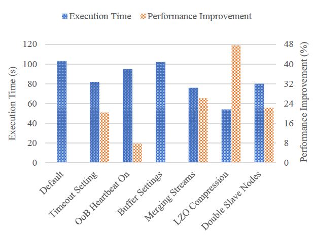 Figure 15: Performance optimization for 2GB+ data cleaning.
The results show three relatively different patterns of optimization effects. First, LZO compression acts as the most effective optimization strategy, and it can improve the performance nearly by 50% when dealing with 2GB+ data. Second, we can expect similar and moderate performance improvement by three individual strategies, such as merging more spilled streams, reducing the timeout value, and doubling the slave nodes. Third, out-of-band heartbeat and buffer settings seem not to be influential optimization strategies in this case.
These different optimization patterns could be closely related to the data characteristics of our application. On one hand, since text data can be compressed significantly [26], our application mostly benefits from the optimization strategy of LZO compression. On the other hand, since the current price traces used in this study are still far from “big data”, the buffer setting could not take clear effects until the data size reaches TB levels.
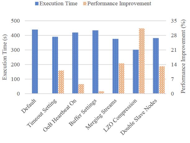 Figure 16: Performance optimization for 5GB+ data cleaning.
5 Related Work
Although the performance advantage of containers were investigated in several pioneer studies [3, 27, 10], the container-based virtualization solution did not gain significant popularity until the recent underlying improvements in the Linux kernel, and especially until the emergence of Docker [28, 29]. Starting from an open-source project in early 2013 [7], Docker quickly becomes the most popular container solution [2] by significantly facilitating the management of containers. Technically, through offering the unified tool set and
API, Docker relieves the complexity of utilizing the relevant kernel-level techniques including the LXC, the cgroup and a copy-on-write filesystem. To examine the performance of Docker containers, a molecular modeling simulation software [30] and a postgreSQL database-based Joomla application [31] have been used to benchmark the Docker environment against the VM environment.
Considering the uncertainty of use cases (e.g., different workload densities and QoS requirements), at this current stage, a baseline-level investigation would be more useful and helpful for understanding the fundamental difference in performance overhead between those two virtualization solutions. A preliminary study has particularly focused on the CPU consumption by using the 100000! calculation within a Docker container and a KVM VM respectively [32]. Nevertheless, the concerns about other features/resources like memory and disk are missing. Similarly, the performance analysis between VM and container in study [33] is not feature-specific enough (even including security that is out of the scope of performance). On the contrary, by treating Docker containers as a particular type of Cloud service, our study considers the four physical properties of a Cloud service [15] and essentially gives a fundamental investigation into the Docker container’s performance overhead on a feature-by-feature basis.
The closest work to ours is the IBM research report on the performance comparison of VM and Linux containers [34]. In fact, it is this incomplete report (e.g., the container’s network evaluation is partially missing) that inspires our study. Surprisingly, our work denies the IBM report’s finding “containers and VMs impose almost no overhead on CPU and memory usage” that was also claimed in [35], and we also doubt about “Docker equals or exceeds KVM performance in every case”. In particular, we are more concerned with the overhead in performance variability.
Within the context of MapReduce clusters, Xavier et al. [10] conducted experimental comparisons among the three aforementioned types of container-based virtual environments, while a set of other studies particularly contrasted performance of OpenVZ with the hypervisor-based virtualization implementations including VMWare, Xen and KVM [3, 27]. The significant difference between these studies and ours is that we focus more on the performance optimization of a container-based MapReduce cluster in a specific application scenario.
Note that, although there are also performance studies on deploying containers inside VMs (e.g., [36, 37]), such a redundant structure might not be suitable for an “apple-to-apple” comparison between Docker containers and VMs, and thus we do not include this virtualization scenario in our study.
6 Conclusions and Future Work
It has been identified that virtualization is one of the foundational elements of Cloud computing and helps realize the value of Cloud computing [38]. On the other hand, the technologies for virtualizing Cloud infrastructures are not resource-free, and their performance overheads would incur negative impacts on the QoS of the Cloud. Since hypervisors that currently dominate the Cloud virtualization market are a relatively heavyweight solution, there comes a rising trend of interest in its lightweight alternative [7], namely the container-based virtualization. Their mechanism difference is that, the former manages the host hardware resources, while the latter enables sharing the host OS. Although straightforward comparisons can be done from the existing qualitative discussions, we conducted a fundamental evaluation study to quantitatively understand the performance overheads of these two different virtualization solutions. In particular, we employed a standalone Docker container and a VMWare Workstation VM to represent the containerbased and the hypervisor-based virtualization technologies respectively.
Recall that there are generally two stages of performance engineering in ECS, for revealing the primary performance of specific (system) features and investigating the overall performance of real-world applications respectively. In addition to the fundamental performance of a single container, we also studied performance optimization of a container-based MapReduce application in terms of cleaning Amazon’s spot price history. At this current stage, we only focused on one factor at a time to evaluate the optimization strategies ranging from setting task timeout to doubling slave nodes.
Overall, our work reveals that the performance overheads of these two virtualization technologies could vary not only on a feature-by-feature basis but also on a job-to-job basis. Although the container-based solution is undoubtedly lightweight, the hypervisor-based technology does not come with higher performance overhead in every case. At the application level, the container technology is clearly more resource-friendly, as we failed in building VMbased MapReduce clusters on the same physical machine. When it comes to container-based MapReduce applications, it seems that the effects of performance optimization strategies are closely related to the data characteristics. For dealing with text data in our case study, LZO compression can bring the most significant performance improvement.
Due to the time and resource limit, our current investigation into the performance of container-based MapReduce applications is still an early study. Thus, our future work will be unfolded along two directions. Firstly, we will adopt sophisticated experimental design techniques (e.g., the full-factorial design) [39] to finalize the same case study on tuning the MapReduce performance of cleaning Amazon’s price history. Secondly, we will gradually apply Docker containers to different real-world applications for dealing with different types of data. By employing “more-than-enough” computing resource, the application-oriented practices will also be replicated in the hypervisor-based virtual environment for further comparison case studies.
Acknowledgment
This work is supported by the Swedish Research Council (VR) under contract number C0590801 for the project Cloud Control, and through the LCCC Linnaeus and ELLIIT Excellence Centers. This work is also supported by the National Natural Science Foundation of China (Grant No.61572251).
- Li, M. Kihl, Q. Lu, and J. A. Andersson, “Performance overhead comparison between hypervisor and container based virtualization,” in Proceedings of the 31st IEEE International Conference on Advanced Information Networking and Application (AINA 2017). Taipei, Taiwan: IEEE Computer Society, 27-29 March 2017, pp. 955–962, https://doi:org/10:1109/AINA:2017:79.
- Pahl, “Containerization and the PaaS Cloud,” IEEE Cloud Computing, vol. 2, no. 3, pp. 24–31, May/June 2014, https: //doi:org/10:1109/MCC:2015:51.
- P. Walters, V. Chaudhary, M. Cha, S. G. Jr., and S. Gallo, “A comparison of virtualization technologies for HPC,” in Proceedings of the 22nd International Conference on Advanced Information Networking and Applications (AINA 2008). Okinawa, Japan: IEEE Computer Society, 25-28 March 2008, pp. 861–868, https://doi:org/10:1109/AINA:2008:45.
- J. Denning, “Performance evaluation: Experimental computer science at its best,” ACM SIGMETRICS Performance Evaluation Review, vol. 10, no. 3, pp. 106–109, Fall 1981, https://doi:org/10:1145/1010629:805480.
- G. Feitelson, “Experimental computer science,” Communications of the ACM, vol. 50, no. 11, pp. 24–26, November 2007, https://doi:org/10:1145/1297797:1297817.
- Li, L. O’Brien, and M. Kihl, “DoKnowMe: Towards a domain knowledge-driven methodology for performance evaluation,” ACM SIGMETRICS Performance Evaluation Review, vol. 43, no. 4, pp. 23–32, 2016, https://doi:org/10:1145/ 2897356:2897360.
- Merkel, “Docker: Lightweight Linux containers for consistent development and deployment,” Linux Journal, vol. 239, pp. 76–91, March 2014.
- Xu, H. Yu, and X. Pei, “A novel resource scheduling approach in container based clouds,” in Proceedings of the 17th IEEE International Conference on Computational Science and Engineering (CSE 2014). Chengdu, China: IEEE Computer Society, 19-21 December 2014, pp. 257–264, https://doi:org/10:1109/ CSE:2014:77.
- Bernstein, “Containers and Cloud: From LXC to Docker to KuBernetes,” IEEE Cloud Computing, vol. 1, no. 3, pp. 81–84, September 2014, https://doi:org/10:1109/MCC:2014:51.
- G. Xavier, M. V. Neves, and C. A. F. D. Rose, “A performance comparison of container-based virtualization systems for MapReduce clusters,” in Proceedings of the 22nd Euromicro International Conference on Parallel, Distributed and Network-Based Processing (PDP 2014). Turin, Italy: IEEE Press, 12-14 February 2014, pp. 299–306, https://doi:org/10:1109/ PDP:2014:78.
- Anderson, “Docker,” IEEE Software, vol. 32, no. 3, pp. 102– 105, May/June 2015, https://doi:org/10:1109/MS:2015:62.
- Banerjee, “Understanding the key differences between LXC and Docker,” https://www:flockport:com/lxc-vs-docker/, August 2014.
- M. Blackburn, K. S. McKinley, R. Garner, C. Hoffmann, A. M. Khan, R. Bentzur, A. Diwan, D. Feinberg, D. Frampton, S. Z. G. M. H. A. H. M. J. H. Lee, J. E. B. Moss, A. Phansalkar, D. Stefanovik, T. VanDrunen, D. von Dincklage, and B. Wiedermann, “Wake up and smell the coffee: Evaluation methodology for the 21st century,” Communications of the ACM, vol. 51, no. 8, pp. 83– 89, August 2008, https://doi:org/10:1145/1378704:1378723.
- Iosup, N. Yigitbasi, and D. Epema, “On the performance variability of production Cloud services,” in Proceedings of the 11th IEEE/ACM International Symposium on Cluster, Cloud and Grid Computing (CCGrid 2011). Newport Beach, CA, USA: IEEE Computer Society, 23-26 May 2011, pp. 104–113, https://doi:org/10:1109/CCGrid:2011:22.
- Li, L. O’Brien, R. Cai, and H. Zhang, “Towards a taxonomy of performance evaluation of commercial Cloud services,” in Proceedings of the 5th International Conference on Cloud Computing (IEEE CLOUD 2012). Honolulu, Hawaii, USA: IEEE Computer Society, 24-29 June 2012, pp. 344–351, https://doi:org/10:1109/CLOUD:2012:74.
- Li, L. O’Brien, H. Zhang, and R. Cai, “A factor framework for experimental design for performance evaluation of commercial Cloud services,” in Proceedings of the 4th International Conference on Cloud Computing Technology and Science (CloudCom 2012). Taipei, Taiwan: IEEE Computer Society, 3-6 December 2012, pp. 169–176, https://doi:org/10:1109/ CloudCom:2012:6427525.
- StackOverflow, “What is the relationship between the docker host OS and the container base image OS?” http://stackoverflow:com/questions/18786209/what-isthe- relationship-between-the-docker-host-os-and-thecontainer- base-image, September 2013.
- Reddit, “Do I need to use an OS base image in my Dockerfile or will it default to the host OS?” https://www:reddit:com/r/docker/comments/2teskf/ do i need to use an os base image in my/, January 2015.
- 19] Z. Li, L. O’Brien, H. Zhang, and R. Cai, “On the conceptualization of performance evaluation of IaaS services,” IEEE Transactions on Services Computing, vol. 7, no. 4, pp. 628–641, October- December 2014, https://doi:org/10:1109/TSC:2013:
- Weinhardt, A. Anandasivam, B. Blau, N. Borissov, T. Meinl, W. Michalk, and J. St¨oßer, “Cloud computing a classification, business models, and research directions,” Business and Information Systems Engineering, vol. 1, no. 5, pp. 391–399, October 2009, https://doi:org/10:1007/s12599-009-0071-2.
- Abhishek, I. A. Kash, and P. Key, “Fixed and market pricing for Cloud services,” in Proceedings of the 7th Workshop on the Economics of Networks, Systems, and Computation (NetEcon 2012). Orlando, FL, USA: IEEE Computer Society, 20 March 2012, pp. 157–162, https://doi:org/10:1109/ INFCOMW:2012:6193479.
- Li, H. Zhang, L. O’Brien, S. Jiang, Y. Zhou, M. Kihl, and R. Ranjan, “Spot pricing in the cloud ecosystem: A comparative investigation,” Journal of Systems and Software, vol. 114, pp. 1–19, April 2016, https://doi:org/10:1016/j:jss:2015:10:042.
- Lu, Z. Li, M. Kihl, L. Zhu, and W. Zhang, “CF4BDA: A conceptual framework for big data analytics applications in the cloud,” IEEE Access, vol. 3, pp. 1944–1952, October 2015, https://doi:org/10:1109/ACCESS:2015:2490085.
- Apache Software Foundation, “Mapreduce tutorial,” https:// hadoop:apache:org/docs/current/hadoop-mapreduce-client/ hadoop-mapreduce-client-core/MapReduceTutorial:html, October 2017.
- Viswanathan, “A guide to using LZO compression in Hadoop,” Linux Journal, vol. 2012, no. 220, August 2012, article no. 1.
- WinZip, “Varying file compression explored,” http:// kb:winzip:com/kb/entry/326/, September 2017.
- Che, C. Shi, Y. Yu, and W. Lin, “A synthetical performance evaluation of OpenVZ, Xen and KVM,” in Proceedings of the 2010 IEEE Asia-Pacific Services Computing Conference (APSCC 2010). Hangzhou, China: IEEE Computer Society, 6- 10 December 2010, pp. 587–594, https://doi:org/10:1109/ APSCC:2010:83.
- Strauss, “Containers – not virtual machines – are the future Cloud,” Linux Journal, vol. 228, pp. 118–123, April 2013.
- Karle, “Operating system containers vs. application containers,” https://blog:risingstack:com/operating-systemcontainers- vs-application-containers/, May 2015.
- Adufu, J. Choi, and Y. Kim, “Is container-based technology a winner for high performance scientific applications?” in Proceedings of the 17th Asia-Pacific Network Operations and Management Symposium (APNOMS 2015). Busan, Korea: IEEE Press, 19-21 August 2015, pp. 507–510, https://doi:org/10:1109/ APNOMS:2015:7275379.
- M. Joy, “Performance comparison between Linux containers and virtual machines,” in Proceedings of the 2015 International Conference on Advances in Computer Engineering and Applications (ICACEA 2015). Ghaziabad, India: IEEE Press, 14-15 February 2015, pp. 507–510, https://doi:org/10:1109/ ICACEA:2015:7164727.
- -T. Seo, H.-S. Hwang, I.-Y. Moon, O.-Y. Kwon, and B.-J. Kim, “Performance comparison analysis of Linux container and virtual machine for building Cloud,” Advanced Science and Technology Letters, vol. 66, pp. 105–111, December 2014, https://doi:org/10:14257/astl:2014:66:25.
- K. Barik, R. K. Lenka, K. R. Rao, and D. Ghose, “Performance analysis of virtual machines and containers in cloud computing,” in Proceedings of the 2016 International Conference on Computing, Communication and Automation (ICCCA 2016). Greater Noida, India: IEEE Press, 29-30 April 2016, pp. 1204–1210, https://10:1109/CCAA:2016:7813925.
- Felter, A. Ferreira, R. Rajamony, and J. Rubio, “An updated performance comparison of virtual machines and Linux containers,” in Proceedings of the 2015 IEEE International Symposium on Performance Analysis of Systems and Software (ISPASS 2015). Philadelphia, PA, USA: IEEE Press, 29-31 March 2015, pp. 171–172, https://doi:org/10:1109/ISPASS:2015:7095802.
- Kozhirbayev and R. O. Sinnott, “A performance comparison of container-based technologies for the Cloud,” Future Generation Computer Systems, no. 68, pp. 175–182, March 2017, https://doi:org/10:1016/j:future:2016:08:025.
- Dua, A. R. Raja, and D. Kakadia, “Virtualization vs containerization to support PaaS,” in Proceedings of the 2014 IEEE International Conference on Cloud Engineering (IC2E 2015). Boston, Massachusetts, USA: IEEE Computer Society, 10-14 March 2014, pp. 610–614, https://doi:org/10:1109/IC2E:2014:41.
- F. Piraghaj, A. V. Dastjerdi, R. N. Calheiros, and R. Buyya, “Efficient virtual machine sizing for hosting containers as a service,” in Proceedings of the 11th World Congress on Services (SERVICES 2015). New York, USA: IEEE Computer Society, 27 June – 2 July 2015, pp. 31–38, https://doi:org/10:1109/ SERVICES:2015:14.
- Angeles, “Virtualization vs. Cloud computing: What’s the difference?” http://www:businessnewsdaily:com/5791- virtualization-vs-cloud-computing:html, January 2014.
- C. Montgomery, Design and Analysis of Experiments, 8th ed. Hoboken, NJ: John Wiley & Sons, Inc., April 2012.