Article Information

Wim P. Krijnen^*,1,2, Lotta Meijerink³, Laurens Zwakhals³, Fanny Janssen⁴, Fons van der Lucht^1,3

¹FAITH Research, Groningen/Leeuwarden, The Netherlands, Research Group Healthy Ageing, Allied Health Care and Nursing, Hanze University of Applied Sciences, Groningen, The Netherlands

²Faculty of Science and Engineering, University of Groningen, Groningen, The Netherlands

³Centre for Health and Society, National Institute of Public Health and the Environment, Bilthoven, The Netherlands

⁴Netherlands Interdisciplinary Demographic Institute – KNAW / University of Groningen, The Hague, The Netherlands

⁵Population Research Centre, Faculty of Spatial Sciences, University of Groningen, The Netherlands

*Corresponding author: Wim P. Krijnen, University of Applied Sciences Sciences, Eyssoniusplein 18, 9714 CE Groningen, The Netherlands.

Received: 17 March 2024; Accepted: 28 March 2024; Published: 19 April 2024

Citation: Wim P. Krijnen, Lotta Meijerink, Laurens Zwakhals, Fanny Janssen, Fons van der Lucht. Modeling Life Expectancy for Municipalities in the Netherlands over of the period 1996-2019. Fortune Journal of Health Sciences. 7 (2024): 231-239.

Abstract

Keywords

Municipality specific life expectancy, Growth trajectory, Four parameter logistic curves, Non-linear mixed effects modeling

Article Details

Introduction

Life expectancy (LE) is a widely used measure to summarize the health of a population. It is used to compare health over time between as well as within countries. In the first decade of this century there was a sharp rise in life-expectancy in most of the western countries [1, 2] due to factors related to improved living conditions, social welfare, education, developments in health care, and prevention of diseases [3-5]. However, since 2015 there is a widespread stagnation of life expectancy reported across various high income EU-countries [6, 7], and, recently a decline of LE in the US [Dobis et al., 2020]. Factors mentioned in the literature for this are influenza peaks, growing socioeconomic health inequalities, as well as economic downturn or austerity [8]. Several factors of influence on LE seem generic, although the combination of these and the influence of still of other factors may very well contribute in different ways to regional or local LE trends in time. LE is often investigated at a macro geographic level e.g. at the scale of a country [9] or a large region [10,11].

In many, but not all, studies a monotonic increase of LE has been found over several years. The latter is frequently investigated by modeling a linear trend, sometimes subdivided into piecewise linear trends. In many cases, however, it seems that a nonlinear increase of LE in time is observed in the data. For such growth processes an S-shape type of trajectory may reveal important information on LE growth rates in time as well as the size of their variations over municipalities. Clearly, such may reveal important additional knowledge on municipality specific growth levels and growth rates in time. By the Dutch law, municipality governments are responsible for local health policies and are obliged to monitor the general health status of their citizens. Due to the current state of affairs, it is unknown at the municipality level whether LE growth trajectories in time have an S-type of shape, how large the differences in LE growth trajectories or LE growth rate are, and to what extend LE growth has stagnated in 2019. More research into local LE growth trajectories is of increasing importance because of decentralizations of governmental tasks in the field  of public health and well-being. The purpose of the current research is to analyze municipality specific LE growth in the Netherlands over a period of two decades by S-shape type of curves.

Methods

Life expectancy is defined as the number of years that a person of a five year age group years is expected to live on the assumption that mortality rates will do change in the future. The rates for the current paper were obtained from the figures of the Causes of Death Statistics Netherlands using persons from the population register of each Dutch municipality. The LE and its variance per municipality for the period 1996-2019 were computed according to the Chiang II method [12, 13], using a moving average over four years. The Chiang method is the most widely accepted method for measuring LE [14]. Estimates for using a moving average over four years were computed for 355 Dutch municipalities, starting at the four year period1996-1999, and ending at 2016-2019, each shifted by one year. The LE moving averages are the data points that serve as input for further non-linear analysis. The analysis of the data is based on functions that have an S-shape type of curve that increases monotonically in time. A suitable family of functions for this is given by the four parameter logistic written as

where t is the variable time in years. It is without loss of generality to assume that the scale  parameter  β₄  is strictly positive. The function value increases monotonically between the lower horizontal asymptote β₂ and the upper asymptote  β₁. That is, the value of the function tends to β₁ if we go forward in time, and it tends to  β₂ if we go backward in time. The parameter  β₃ represents the midpoint of growth in time, where the function attains the average of the two horizontal asymptotes. At the midpoint, the curve attains its inflection point at which the growth rate is maximal. The growth rate can be evaluated by the first order derivative of f at any time point t. In order to adapt the curve to municipality specific LE data we need to use a model with random effects. Specifically, for municipality j at time point  t_i  we consider the model

where y_ij  is the LE for municipality j at time point t_i, and ε_ij the normally distributed error with mean zero and variance  σ² . The non-linear model is mixed in containing fixed parameters that hold for the population and random parameters that adapt for each municipality. The parameters become estimable by maximum likelihood after constraining the random effects to have mean zero [15, 16]. We employ the likelihood ratio approach as well as information indices [17] to test the hypothesis that the error terms have a moving average of order 1 or 2 type of correlation structure,  known as ARMA(0,2), as well as the additional hypothesis that the sample LE variances form a co-variate for the error variance of the municipalities. In this way we find better models after starting with a relative simple model. Maximum likelihood of the four-parameter mixed model given the data yields estimates of the fixed parameters  β₁,β₂,β₃ ,β₄  and the random parameters b_1j,b_2j,b_3j. By inserting the corresponding parameters into the function f  the best approximating curve for each municipality is obtained. From these, several informative quantities can be computed in order to characterize and compare LE growth trajectories for the municipalities over the study period. The level of the upper horizontal asymptote (β₁+b_1j) indicates the “end” level of the municipality specific LE growth, up to the error in the LE measurements relative to the curve and the time span of the LE data. Similarly, the lower horizontal asymptote  (β₂+b_2j)   indicates the “begin” level. The difference between the two horizontal asymptotes gives the municipality specific LE growth over the study period. Such a difference is in line with the data if the S type of cycle is completed by a municipality. In case the cycle is not completed an asymptote may occur below or above the data.

The first order derivative at any time point gives the municipality specific LE growth rate. Evaluated at the midpoint t = (β₃+b_3j) this gives the specific maximal growth rate during the process for municipality j = 1,··· ,N. If the first order derivative is close to zero at the end of the study, then this indicates complete stagnation of LE growth. If the first order derivative is positive, then a further LE increase in the short term can reasonably be expected. The LE growth rate at the end of the study will be interpreted to evaluate the degree in which stagnation of LE growth occurred. The root of the mean squared error

For municipality j = 1,··· ,N gives its prediction error. The unit of measurement of the RMSE is in years of LE. If the prediction error is small for a municipality, then all LE data values y_ij  are close to the four-parameter logistic curve _ij  and several meaningful conclusions can be drawn. If, on the other hand, the prediction error is very large, then this obviously would complicate drawing meaningful conclusions for the  specific municipality. Furthermore, we may see the difference in horizontal asymptotes relative to the RMSE, as the ``signal to noise’’ ratio. If the latter is close to one, then the LE values may be more or less randomly spread around its mid point level. On the other hand, if the signal to noise ratio is large, then meaningful conclusions are possible.

The distribution of various quantities of the municipalities are summarized by violin plots. Visual inspection of these quickly reveal important information on their distribution, variation, degree of symmetry, and presence of outliers. Two geographical maps of the municipalities in the Netherlands are given to illustrate the maximal (midpoint) growth rate and that at the end of the study. Out of all plots over the municipalities of the LE data in time a few are selected to illustrate the gain insight into LE trends for the bigger cities, municipalities with high or low levels of LE trends in time, and municipalities with a high growth rate. The asymptotes are represented as horizontal lines.

Results

Figure 1: Violin plot of LE data in time from 1996 to 2019 over 354 municipalities.

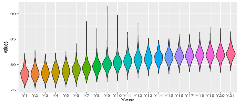
Statistics Netherlands kindly provided the mortality data for the age cohorts 0, 1-24, 25-44, 45-54, 55-64, 65-69, 70-74, 75-79, 80-84, and 85 or older. From these we computed the LE values according to the Chiang II method [12, 13] and the 4-year moving averages. The computations take merging of municipalities as well as migrations into account on the basis of membership of age cohort. The 4-year moving averages make the LE values more robust against single outliers, which are less representative for longer trends. This yielded 21 LE determinations for each of the 355 municipalities over the period 1996 and 2019. The violin plot of the LE data per time period from 1996-1999 to 2016-2019 over the municipalities is given in Figure 1. There is a clear trend observable that the LE distributions in time roughly increase according to an S-shape type of pattern. That is, in the first six years the violin plots are more or less at the same level, next there is an increase observable during a period of about ten years, followed by a period of five years where the LE levels stabilize. The distributions of LE levels over the municipalities are fairly, but not completely, symmetric with a very few number of extreme outliers. From this we conjecture that similar four parameter logistic LE trends also hold for individual municipalities, reason for which this is given a closer investigation in the below.

Table 1: Statistical testing of the models without error structure, those with moving average of order 1 and 2, and additionally with an error variance co-variate from the data, where the p-value corresponds to likelihood ratio against the previous.

Table 2: Marginal t-testing of the fixed four parameter logistic model over the 21 LE data points from the 354 municipalities with standard error (SE) and lower and upper limits of the 95 percent confidence intervals (CI).

The four-parameter logistic model with random effects was estimated by maximum likelihood. Unfortunately, a single municipality (Rozendaal) had to be excluded from the analysis due to extreme variations in the data. The model without error structure on the residuals is tested by likelihood ratio against the model with moving average of order 1, see Table 1. The former is clearly rejected by the ARMA(0,1) model. However, the latter model is clearly rejected by the ARMA(0,2) model, which consecutively is rejected by the ARMA(0,2) model with the co-variate on the error variances. The encountered differences in the information criteria AIC and BIC, as well as in the log-likelihood are very large and completely in line with the conclusions from likelihood ratio testing. Obviously, this is line with the moving average structure of the data and the heterogeneity in error variances over the municipalities. For the final model the estimated ARMA(0,2) moving average parameters are 0.62 with CI (0.55, 0.69), 0.31 with CI (0.27, 0.36), the power of variance parameter is 0.49 with CI (0.47, 0.51), and the within group standard error is 0.94 (=  ) with CI (0.89, 0.98). The estimated fixed parameters of the four parameter logistic model and their corresponding p-values are given in Table 2. Marginal t-testing of the fixed parameters indicates that these are significantly different from zero. The difference of 4.1 years between the lower and upper horizontal asymptotes may be interpreted as the average municipality growth in LE over 21 years. The estimated time to maximal growth (midpoint) is 9.1 years, which by taking the middle 1998 of the period 1996 to 1999 as the start of the study, comes down to February 2007.

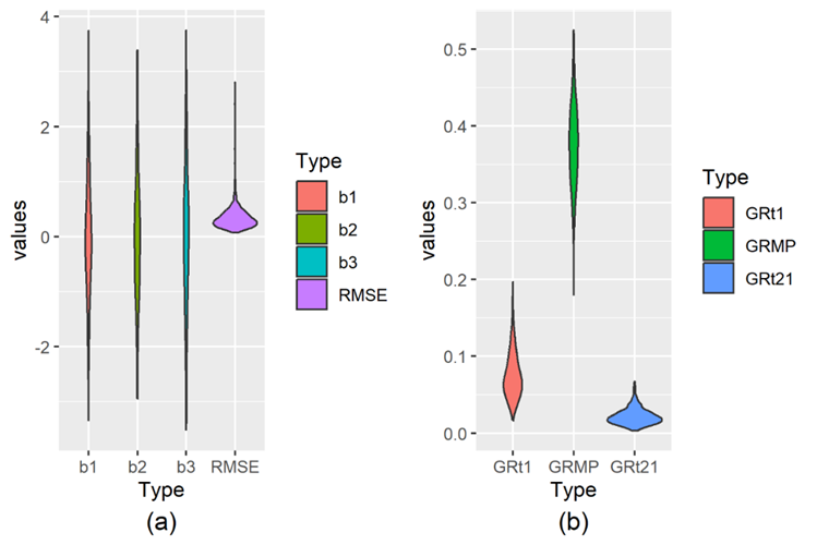
The distributions of the centered random effects for the municipalities are summarized by violin plots in the left hand side of Figure 2. Almost all upper and lower asymptotes fall within a range of about 6 years, which is in line with the LE distributions per time point. The distribution of the midpoint random effects is similar to that of the horizontal asymptotes. Adapted for the municipalities the lower horizontal asymptotes have mean 78.0 years of LE, with 95 percent within the interval (76.0, 80.1), and 75.1 and 81.5 years of LE as the smallest and largest, respectively. The upper horizontal asymptote has mean 82.2 years of LE, with 95 percent within the interval (80.0, 84.4), with 78.8 as the smallest and 86.0 as the largest. The mean difference in horizontal asymptotes is 4.2 years of LE, with 95 percent of the differences within the interval (3.0, 5.4), with 1.97 as the smallest and 5.8 as the largest. The violin plot of the RMSE values is given in the left hand side of Figure 2. It can be observed that the prediction error is relatively small compared to the size of the differences in the random parameters. In the absolute sense, it can be observed that the RMSE is large for a tiny fraction of the municipalities. Moreover, the RMSE is smaller than 0.29 for 50% of the municipalities and smaller than 0.55 for 90% of the municipalities. That is, for a large fraction of the municipalities the LE data are close to their specific S-shape curve, so that it provides useful information on the LE growth process in time. More in the relative sense, the signal to noise ratio, defined by the difference in horizontal asymptotes and the RMSE, is larger than 5 for 97.5% and larger than 9 for 80% of the municipalities. The violin plots at the right hand side of Figure 2 summarize the distribution of the LE growth rates of the municipalities at the start, midpoint, and the end of the study. The 95 percent of the obtained growth rates for the municipalities at the start of the study are within the interval (0.03, 0.14), for those at the midpoints this is (0.27, 0.49), and for those at the end of the study this is (0.007, 0.047). Furthermore, the mean growth rate increased from 0.076 at year 1996 to a maximum of 0.3761 at the midpoint, and, next, it decreased to 0.0219 at 2019, the end of the study. The sizes of the growth rate clearly increased with time to midpoint and next decreased to almost zero. Similarly, the variation in growth rate increased to rather large values at the mid point, whereas the variation became rather small at the end of the study. That is, the municipalities became much more homogeneous at the end of the study, generally showing stagnation of LE growth.

Figure 2: Violin plots of the distribution of the municipality random effects for the upper (b1), lower (b2) asymptote and midpoint (b3), and the root-mean-square error (RMSE) to the left in (a).  Violin plots of the distribution of municipality LE growth rate at the start of the study 1996 (GRt1), the mid-point (GRMP) and at the end of the study 2019 (GRt21),  to the right in (b).

For completeness it may be noted that the correlation between the lower horizontal asymptote and the maximum growth rate is -0.21 (95% CI -0.31; -0.11), so that there is a weak tendency for municipalities with a higher begin level to grow less. The correlation between the end level and the maximal growth rate is 0.35 (95% CI 0.25; 0.43), reflecting a weak tendency for municipalities with a higher maximal growth rates to reach a higher end level over the study period.

Figure 3: Map with maximum LE growth rate over 1996-2019 for the municipalities in the Netherlands.

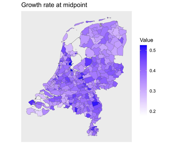
The geographical map of the municipalities in the Netherlands with the maximum growth rates at the midpoint is given in Figure 3, where the color intensity indicates the growth rate for each municipality. The municipalities on the North East tend to have lighter colors indicating lower growth rates at the midpoint. The observed frequencies corresponding to the maximum growth rate were that 2 municipalities are lower than 0.2, 24 within the interval (0.2,0.3], 208 within (0.3,0.4], 114 within (0.4,0.5], and 6 within (0.5,0.525]. For the municipalities with the smallest maximum growth rate it would take 5 years and for the largest it would take 2 years for the LE to increase by one year. This clearly illustrates drastic differences in maximum LE growth rate among Dutch municipalities.

Figure 4: Map with LE growth rate at end point of the study 2019 for municipalities in the Netherlands.

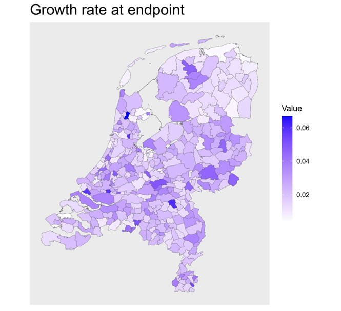
The geographical map with intensity of color indicating growth rate at the end of the study is given by Figure 4. There are 180 municipalities with a growth rate within the interval (0,0.02], 153 within (0.02,0.04], 19 within (0.04,0.06], and 2 within (0.06,0.07]. For the smallest it would take more than 50 years to increase the LE by one year and for the largest it would take 15 years to increase the LE by one year. The variation in growth rate at the end of the study is considerably smaller than at the mid point (see also Figure 2). That is, the municipalities are rather homogeneous in their stagnation of LE growth at the end of the study. The stagnation of LE growth is clearly visible from a comparison of the geographical maps in Figure 3 and 4.

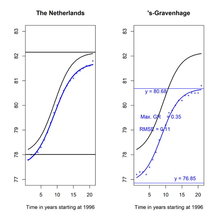
The curve that corresponds to the estimated parameters in Table 2 serves in the below as a reference representing the average municipality. The graph of this curve and its horizontal lines are given at the left hand side of Figure 5 together with the curve from the country-wise LE values in the Netherlands. It can be observed that at the start of the study the growth rate was small, that it increased until the midpoint, and, next, that it decreased to almost zero at the end of the study. The fitted parameters from the country wise LE data are 81.74 for the upper asymptote, 77.48 for the lower asymptote, 9.02 for the midpoint, and 3.08 for the scaling parameter. The RMSE of 0.06 for the fitted curve to the country wise LE data is very low, indicating that the LE values are very close to the curve. The shapes of the two curves are remarkably similar with that for the country shifted downward by approximately 0.44 years compared to the average municipality.

Figure 5: Trend in LE data from the Netherlands with its 4 parameter logistic curve in blue compared with the average municipality curve and its upper and lower asymptotes at left hand side. Trend in LE data over 1996-2019 with the four parameter logistic curve for the municipality ’s-Gravenhage (Den Hague), right hand side.

The LE data and the estimated curve of curve for the municipality ’s-Gravenhage, also known as Den Hague, is given the right hand side of Figure 5. It can be observed that its prediction error is small and that the curve fits the LE data quite well. The curve is very similar in form to that of the average municipality, albeit it is shifted about one year downward due to the generally lower LE values in Den Hague throughout the study period. The other three major cities in the Netherlands, Amsterdam, Rotterdam, and Utrecht, have very similar LE growth trajectories to that of Den Hague. The LE level in the major cities is about one year below the average LE curve over all municipalities.

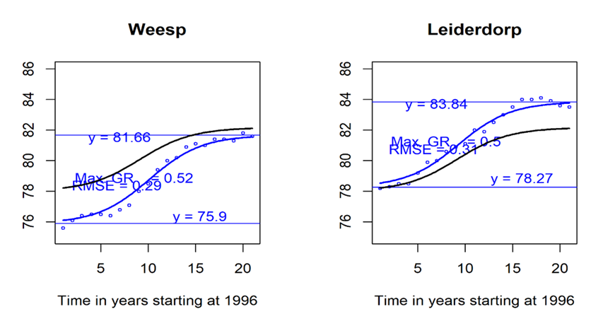
The total growth in LE during the study period measured by the difference in horizontal asymptotes varies between the municipalities quite substantially. The smallest total LE growth rate of 2 years was observed for the municipality Vlissingen. Furthermore, there are 6 municipalities with a total growth within the interval (2,3], 134 within (3,4], 184 within (4,5], and 28 of more than 5 years. The total growth is closely related to the size of the maximal growth rate. To illustrate the effect of a large growth rate, the LE data with the estimated graphs of two municipalities are visualized. In particular, for the municipality Weesp and Leiderdorp the LE data with their S-shape curve and horizontal lines are given in Figure 6. It can be observed that the difference in LE levels compared with the average municipality is reduced for Weesp and increased for Leiderdorp during the study period. The larger growth rate than average is clearly visible from the steepness of the curves. Because growth rates at the end of the study are near zero, the upper lines (asymptotes) reflect the LE level at the end of the study quite well. There are 7 municipalities with end LE level in the interval (78,80], 154 within (80,82], 176 within (82,84], and 17 within (84,86].

Figure 6: Trend in LE data over 1996-2019 with four parameter logistic curve for municipality Weesp to the left and Leiderdorp to the right in blue and the average municipality in black.

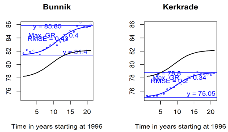
To illustrate large differences in LE levels, the data and curves of two municipalities are visualized. In particular, for the municipalities Kerkrade and Bunnik the LE data with S-shape curve and horizontal lines (asymptotes) is given Figure 7. Compared with the average municipality curve the Bunnik LE levels are about three years higher and those of Kerkrade three years lower throughout the study period. Bunnik and Kerkrade exemplify municipalities, respectively, with about 11,000 and 45,000 inhabitants, to have relatively small prediction errors, given their size.

Figure 7: Trend in LE data over 1996-2019 with four parameter logistic curve for municipality Bunnik to the left and Kerkrade to the right in blue and the average municipality in black.

Conclusions and Discussion

Almost all Dutch municipalities have an S-shape type of growth trajectory over the period 1996 - 2019, including those with a size as small as 10,000. On average, the LE growth rate over the municipalities increased to 0.38 per year in February 2007 and drastically decreased to 0.02 per year in 2019. This stagnation in LE growth is omnipresent over the Dutch municipalities. The four big cities in The Netherlands have about one year lower LE levels compared to the average municipality throughout the study period of 21 years. The LE levels between municipalities differs to up to six years. The large differences in growth rate among the municipalities cause an increase or decrease of the LE level compared to the average.

Our results obtained at the municipality level are in line with the previous country wise type of LE findings from the literature that state a sharp increase of LE in 2007 in most of the high income western countries [1, 2] followed by a stagnation of life expectancy growth [7, 18-20]. The omnipresent stagnation of LE growth among Dutch municipalities indicates that the previous findings on stagnation are not the results of an average that balances positive with negative LE growth. The characteristics of the growth trajectories and their comparisons are useful for the general public, and for local, regional, as well as country wise policymakers. The study made trends of municipality LE growth as well as differences rather explicit and shows how these can be monitored. In addition, the patterns of lower or higher levels of LE are rather stable for certain municipalities. The differences between municipalities to up to six years of LE seems rather large and deserves attention. Several researchers have provided evidence at the country level for factors of LE growth such as prevention for cerebrovascular diseases, traffic accidents [1], smoking [2], combination of smoking, obesity, and alcohol abuse [4], as well as causes for evidence of stagnation of LE growth such as austerity [8, 21].

A reasonable explanation for the country wise S-shape curve to be lower by 0.44 years compared to the average municipality seems that larger municipalities tend to have lower LE levels and this gets more emphasized in the national LE due to their larger populations. The resemblance of the shape of the curve for the average municipality and for the country as a whole may be seen as further evidence for the validity of the approach. What is new in this study is the application of the mixed non-linear model based on the four parameter logistic curve to fit LE data over a period of two decades at a low level of aggregation, namely municipalities. The method made several concepts related to LE rather explicit. This holds for municipality specific concepts such as the starting level of LE, the end level of LE, total LE growth, the growth rate at any time point, as well as stagnation of growth. In particular, the growth rate defined as the first order derivative of the four parameter logistic curve is new to LE research. For many municipalities the deviations around the S-shape curve are much smaller than the systematic variation between the start and the end of the study. In particular, the four big cities have a large signal to noise ratio. If such municipalities also went through a complete logistic cycle, the upper line clearly summarizes the end LE level the S-shape LE growth process. If underlying causes of LE growth stay equal, then the observed stagnation will continue in the near future. Prediction of future LE growth obviously becomes uncertain in case of a (drastic) change of circumstances caused by e.g. a pandemic [22], although the size of such changes is to be scientifically determined by future research. For municipalities with large RMSE, prediction of future LE levels hold with less certainty or may even be impossible. [23] suggested, among other things, a sensitivity to cohort and tempo effects leading to accidental or rather random fluctuations. For municipalities with high signal to noise ratios the certainly of the LE trend increases considerably in comparison to single LE levels.

More than one thousand parameters were estimated by the numerical optimization procedure to obtain the maximum likelihood estimates of the four parameter logistic mixed model. Leaving out the random scale parameters seems not a limitation, since the differences in steepness in the data are modeled quite precisely. The above approach is not perfect in the sense that it yields some significant autocorrelations between the residuals indicating these to contain some correlated noise. The possibilities to repair this by further modeling is somewhat limited by the restricted number of time points and, additionally, it is unlikely that such would change the estimated logistic parameters that approximate the municipality specific LE data. A disadvantage of the four parameter logistic model is that is monotonically (de- or) increasing in time, which may not hold for all LE trends of the municipalities in time. A more flexible alternative is to use mixed modeling with cubic or quartic polynomials so that the curve can have a local maximum or minimum. Yet, another alternative is to use mixed modeling with robust cubic splines, where the robustness guards against over flexibility due to outliers. These alternatives would provide LE trend approximations by differentiable functions for which the concept of LE growth becomes available for each time point. For such alternatives it is of importance to keep the balance between over- and under-fitting the data. The above approach does not include regression type of variables that explain the characteristics of the LE growth trajectories for municipalities such as size of the maximum growth rate or the LE levels at the end of the study. Such quantities, however, can easily be extracted and subjected to further analyses by standard regression methods.

Several researchers have provided evidence at the country level for factors of LE growth such as prevention for cerebrovascular diseases, traffic accidents [1], smoking [2], combination of smoking, obesity, and alcohol abuse [4], as well as causes for evidence of stagnation of LE growth such as austerity [8, 21]. The above characteristics of the LE growth trajectories for municipalities opens new directions for research, for instance, into determinants of the size of the maximum growth rate or the level of the upper asymptote. Other directions are the possibility to search for municipalities which have a low/high begin level as well as a small/large value of maximal growth and the further investigation of determinants for these.

References

1. Bahk J and Jung-Choi K. The contribution of avoidable mortality to the life expectancy gains in korea between 1998 and 2017. International journal of environmental research and public health 17 (2020): 6499.
2. Cao X, Hou Y, Zhang X, Xu C, Jia P, Sun X, et al. A comparative, correlate analysis and projection of global and regional life expectancy, healthy life expectancy, and their gap: 1995-2025. Journal of Global Health 10 (2020).
3. Janssen F. The role of smoking in country differences in life expectancy across Europe, 1985-2014. Nicotine and Tobacco Research 23 (2021): 152-160.
4. Janssen F, Trias-Llimos S, and Kunst AE. The combined impact of smoking, obesity and alcohol on life-expectancy trends in Europe. International Journal of Epidemiology (2021).
5. Mesceriakova-Veliuliene O, Kalediene R, Sauliune S, and Urbonas G. Inequalities in life expectancy by education and its changes in lithuania during 2001-2014. Medicina 57 (2021): 245.
6. Ho JY. and Hendi AS. Recent trends in life expectancy across high income countries: retrospective observational study. BMJ 362 (2018).
7. Raleigh VS. Trends in life expectancy in EU and other OECD countries: Why are improvements slowing? (2019).
8. McCartney G, Fenton L, Minton J, Fischbacher C, Taulbut M, Little K, et al. Is austerity responsible for the recent change in mortality trends across high-income nations? A protocol for an observational study. BMJ open 10 (2020): e034832.
9. Doctors O. In health at a glance 2021: OECD indicators (2021).
10. van Raalte, A. A., Kl¨usener, S., Oksuzyan, A., and Grigoriev, P. (2020). Declining regional disparities in mortality in the context of persisting large inequalities in economic conditions: the case of Germany. International journal of epidemiology, 49(2):486-496.
11. Vierboom YC, Preston SH, and Hendi AS. Rising geographic inequality in mortality in the united states. SSM-population health 9 (2019): 100478.
12. Chiang CL, Organization WH, et al. Life table and mortality analysis (1979).
13. Toson B and Baker A. Life expectancy at birth: Methodological options for small populations. Office for National Statistics London (2003).
14. Lo E, Vatnik D, Benedetti A, and Bourbeau R. Variance models of the last age interval and their impact on life expectancy at subnational scales. Demographic Research 35 (2016): 399-454.
15. Seber G and Wild C. Nonlinear Regression. Wiley Series in Probability and Statistics. Wiley (1989).
16. Pinheiro J and Bates D. Mixed-effects models in S and S-PLUS. Springer Science & Business Media (2006).
17. Konishi S and GK. Information Criteria and Statistical Modeling. Springer Series in Statistics. Springer (2008).
18. Kim T, Bahk J, Lim HK, and Khang Y-H. Stagnation of life expectancy in Korea in 2018: A cause-specific decomposition analysis. PloS one 15 (2020): e0244380.
19. Murphy M. Recent mortality in Britain: a review of trends and explanations. Age and Ageing 50 (2021): 676-683.
20. Ramsay J, Minton J, Fischbacher C, Fenton L, Kaye Bardgett M, Wyper GM, et al. How have changes in death by cause and age group contributed to the recent stalling of life expectancy gains in Scotland? comparative decomposition analysis of mortality data, 2000-2002 to 2015-2017. BMJ open 10 (2020): e036529.
21. Currie J, Boyce T, Evans L, Luker M, Senior S, Hartt M, et al. Life expectancy inequalities in Wales before covid-19: an exploration of current contributions by age and cause of death and changes between 2002 and 2018. Public Health 193 (2021): 48-56.
22. Aburto JM, Sch’oley J, Kashnitsky I, Zhang L, Rahal C, Missov TI, et al. Quantifying impacts of the covid-19 pandemic through life-expectancy losses: a population-level study of 29 countries. International journal of epidemiology 51 (2022): 63-74.
23. Luy M, Di Giulio P, Di Lego V, Lazarevic P, and Sauerberg M. Life expectancy: frequently used, but hardly understood. Gerontology 66 (2020): 95-104.
24. Dobis E, Stephens H, Skidmore M, and Goetz S. Explaining the spatial variation in American life expectancy. Social Science & Medicine 246 (2020): 112759.