


Introduction
Sea ice in the Arctic and the Antarctic plays a well-recognized part in climate and ocean modelling. One aspect of some interest is the thermal response of sea ice to solar radiation (e.g. Reference Flato and BrownFlato and Brown, 1996; Reference Key, Silcox and StoneKey and others, 1996; Reference Hanesiak, Barber and FlatoHanesiak and others, 1999). In temperature measurements taken to calculate the thermal conductivity we have noted (Reference McGuinness, Trodahl, Collins and HaskellMcGuinness and others, 1998; Reference TrodahlTrodahl and others, 2000) daily oscillations consistent with solar heating. The accuracy and resolution of these measurements provide a direct measurement of the thermal effect of solar radiation. A preliminary analysis of the observed thermal response to solar heating appears in Reference TrodahlTrodahl and others (2000), and we seek to extend this work here. In particular, we seek to analyze more accurately the conductive and volumetric heating effects.
In this paper we report on the temperature data gathered in McMurdo Sound, Antarctica, we describe the Monte Carlo scattering simulations performed to calculate the absorbed solar power as a function of depth in sea ice, we outline and solve a mathematical model for the diffusion of heat in sea ice that incorporates solar heating as a distributed source term, and finally we compare and discuss the results.
Temperature Data
Thermistor arrays frozen into first-year, landfast sea ice in McMurdo Sound in 1996 and 1999 yield hourly temperature measurements at 20 depths spaced 0.1 m apart during winter and spring. The chosen locations, one about 1 km off Arrival Heights, and the other in the lee of Big Razorback Island off Cape Evans, had little snow accumulation. The ice in both locations grows to a thickness of > 2 m in winter.
Recorded temperatures are plotted against time in Figures 1 and 2. Each line of data corresponds to one thermistor, so that the higher temperatures correspond to the deeper (warmer) thermistors. The Omega 44031 thermistors used are calibrated and uniform to 0.1 °C, but their potential resolution is ∼0.001 °C. Actual uncertainty is in practice ∼0.01 °C.
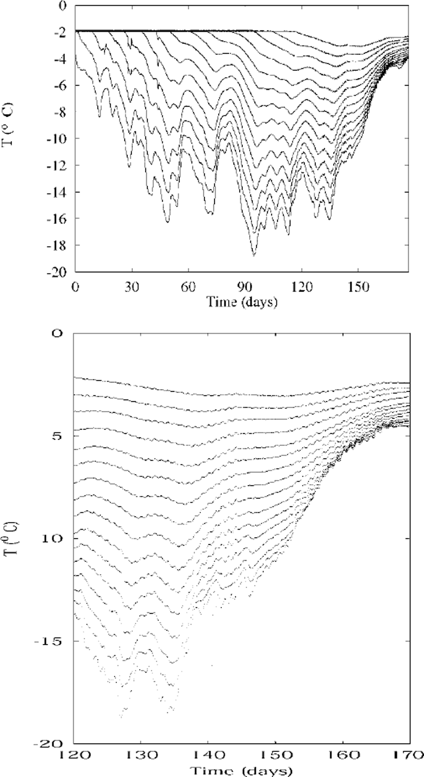
Fig. 1. Temperatures measured in 1996, plotted against time. each line is the temperature recorded by one thermistor at a constant depth. the upper plot shows temperatures during winter and spring at depths 0.7−2.0 m, with the coldest temperatures being from the 0.7 m deep thermistor. the lower plot shows more detail during spring, and is for depths 0.5−2.0 m. day zero is 12 june.
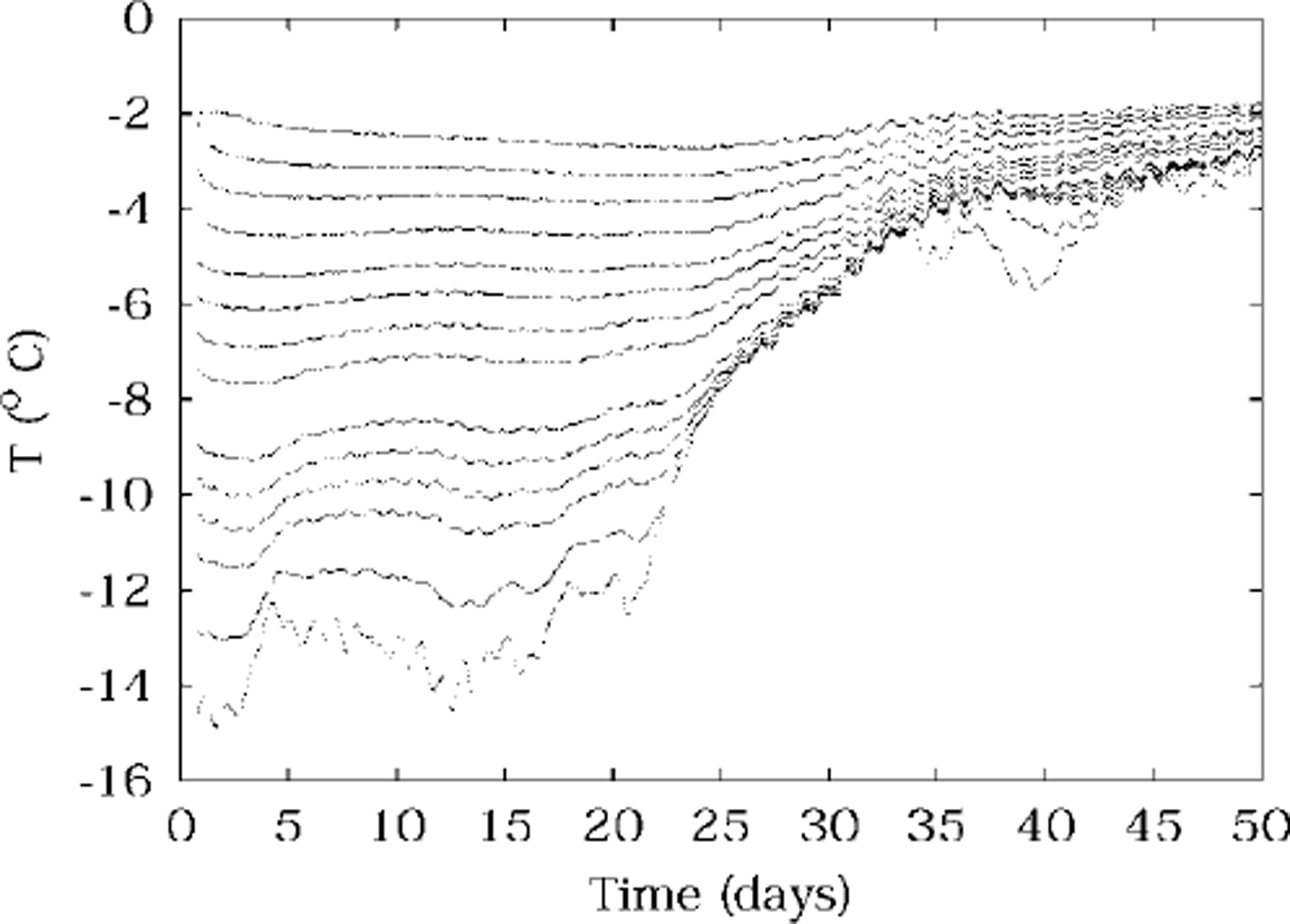
Fig. 2. Temperatures measured in spring 1999, plotted against time, from thermistors at depths 0.4−1.9 m. data from 0.6 and 1.1m are missing, due to faulty thermistors. day zero is 14 october.
Of some concern is the possibility that the observed temperature oscillations are due to the sun directly heating the thermistor string, rather than to variations in ice temperature. The direct heating of the thermistors by sunlight has been modelled in Reference TrodahlTrodahl and others (2000) and was found to be negligibly small in amplitude. Furthermore it would be in phase with the sun, and this is not observed in our data.
The temperature data show changes forced by variations in air temperature, and also during some periods in spring a smaller, faster (daily) oscillation can be seen superimposed on the slower changes, which we assume is due to solar forcing. It is this solar forcing which we investigate further in this paper.
There are periods during spring when no solar forcing is visible; we believe this is when cloud obscures the sun.
Monte Carlo Scattering
The optical energy absorbed per unit volume at any depth z in the ice is given by the product of the average radiance and the absorption coefficient. However, the average radiance is not easily determined within the very successful Monte Carlo models we have developed on the basis of light-spreading measurements. We have thus adapted these models to simulate the absorption process.
The core element in the Monte Carlo models is the tracing of many randomly scattered light paths for rays impinging on the surface. The effects of scattering are modeled by a depth-dependent scattering length (mean-free-path) whose magnitude and depth dependence are chosen to reproduce experimentally-determined beam-spreading profiles (Reference Haines, Buckley and TrodahlHaines and others, 1997). In the present case, where we wish to simulate the heat absorbed in the ice, we follow the paths through many layers of thickness Δz centred at depths ![]() and record for each traverse j of a ray through that layer the path length li spent in the layer, binned by the total path Lj that the ray has followed before reaching that level. Then the absorbed power per unit volume at that depth due to a flux FλΔλ falling on the surface in wavelength bands A to A + AA, and summed over all wavelengths, is
and record for each traverse j of a ray through that layer the path length li spent in the layer, binned by the total path Lj that the ray has followed before reaching that level. Then the absorbed power per unit volume at that depth due to a flux FλΔλ falling on the surface in wavelength bands A to A + AA, and summed over all wavelengths, is

where n is the number of rays used in the Monte Carlo model, and kλ IS the absorption coefficient for pure ice in the wavelength band λ to λ + Δλ. The wavelength range used is 300−1400 nm. The specific models, specified by the depth-dependent scattering length, include three of those determined for McMurdo Sound first-year ice (Reference Haines, Buckley and TrodahlHaines and others, 1997). We note that they all display a strongly scattering surface layer and a more weakly scattering interior, and these features will be seen below to influence the light-absorption profiles. Such a two-layer structure is also apparent in studies of Arctic first-year sea ice (e.g. Reference Perovich, Roesler and PegauPerovich and others, 1998).
The base ten logarithms of the resulting power densities are plotted against depth in Figure 3. The models used range from the most transparent (curve c), through an intermediate case (curve a), to the most opaque or turbid (curve b) of those developed by Reference Haines, Buckley and TrodahlHaines and others (1997). The powers are for midday during spring, and are used as an estimate of the peak-to-peak variation of solar power. They are used in the distributed source term in the heat-conduction modelling in the next section, and they are the most important factor in determining the amplitudes of temperature oscillations in the ice due to solar radiation penetration.

Fig. 3. The base ten logarithm of solar power absorbed per unit volume (j m3), vs depth in the sea ice, calculated by monte carlo scattering, and using scattering lengths fitted to 1986 experiments. the labels a, b, c on the curves correspond to cases 86a, 86b and 86c, respectively, used by Reference Haines, Buckley and TrodahlHaines and others (1997). the power is that at midday on a typical spring day in mcmurdo sound.
Mathematical Modelling
We model the temperature field in the sea ice with a one-dimensional heat-diffusion equation. Heating by solar radiation is included as a distributed source term, as calculated in the previous section. The equation describing the conduction of heat in the sea ice is
where the diffusivity is

and the solar driving term is
where temperature is the real part of 6 in °C, θ is a complex-valued function of depth z and time t, k is thermal conductivity, here taken to be 2 W m−1 k−1 p is the density of the sea ice, and p is the solar power absorbed per unit volume (J m−3) of sea ice. A complex-valued 6 is computationally convenient for analyzing oscillations. Depth z is zero at the upper ice/air interface, and has been rescaled to give z = 1 at the lower ice/water interface, using the factor l, the total ice thickness, which is taken to be l = 2 during spring.
The factor (1 + aeiwt) accounts for the daily variation in amplitude as the sun rises and falls, with frequency ω = 2π rad d−1. a has modulus one, which corresponds to the sun just touching the horizon overnight. The argument of A sets the zero of time with respect to the sun’s periodic behaviour. c(θ) is the temperature-dependent heat capacity per unit mass of sea ice (kJ kg−1 ˚C−1), and we use the empirical formula (Reference SchwerdtfegerSchwerdtfeger, 1963; Reference OnoOno, 1966; Reference YenYen, 1981)

where s is the salinity in practical salinity units (psu) of the sea ice, here taken to be 5.5 psu.
The boundary condition used at the sea/ice interface where z = 1 is to fix the temperature at the value θ0 = −1.8°C.
For the boundary condition at the upper ice surface z = 0, a Newton-type heat loss is used, with the temperature gradient at the surface proportional to the difference between the ice temperature and the air temperature,
where a is some positive constant. If a = 0, the ice is perfectly insulated from the air. If α → ∞, the ice temperature at the surface is equal to the air temperature there. Equation (6) corresponds to the sensible-heat flux, mentioned, for example, in Reference Zeebe, Eicken, Robinson, Wolf-Gladrow and DieckmannZeebe and others (1996). Their work suggests the value α ≈ 12 at average wind speeds in McMurdo Sound.
This boundary condition may appear crude compared, for example, with that of Reference Zeebe, Eicken, Robinson, Wolf-Gladrow and DieckmannZeebe and others (1996), but incoming and outgoing radiation effects at the upper surface are already accounted for explicitly by the Monte Carlo simulations through the source term p(z), for wavelengths in the range 300−1400 nm, and hence are not needed in the boundary condition. Radiation at wavelengths of > 1400 nm is ignored here, because we see very little power in the spectrum of the solar radiation striking the ice surface above 1400 nm. We also ignore latent-heat effects at the ice/air interface. For the Weddell Sea, latent-heat fluxes have been estimated (Reference EickenEicken, 1992) to be about a quarter of the size of the sensible-heat fluxes. Furthermore, we find in the following sections that the oscillatory solar forcing solutions are not very sensitive to the boundary condition used at the upper surface.
Asymptotic analysis
The model equation (2) for temperature is non-linear, and as it stands it is difficult to extract information about solution responses to penetrating solar radiation. However, large temperature variations on time-scales of the order of lweek or more (slow time), and smaller daily temperature oscillations (fast time), are visible in the temperature data presented in Figures 1 and 2. Hence we will make progress by proceeding to analyze the daily small-scale changes as perturbations on the longer-term trends.
We seek a temperature expansion in the form
where (following, e.g., Reference Kevorkian and ColeKevorkian and Cole, 1981) we are using a multiple time-scales analysis, with t a fast time, ∊ a small parameter, and τ = et a slow time-scale. Note that we are explicitly taking the leading behaviour ^ to be slowly varying in time. If we choose q to also be of size ∊, we find the background temperature ϵ solves the steady-state problem
which has a solution of the form
Substituting this into the boundary conditions then gives

The temperature at the top of the sea ice (z = 0) is

Note that as α → ∞, ϵt op → 0air, as expected since large a corresponds to good thermal contact between ice and air. The leading temperature behaviour V is linear in z, taking the values 90 at z = 1 and ϵtop at z = 0.
The ![]() problem is
problem is

where d = d(ϵ(τ, z)) and q = q(z, ϵ(τ, z)).
This is a linear partial differential equation for v. The righthand side consists of oscillatory and non-oscillatory forcing terms, and we are only interested in the oscillatory behaviour of v. Hence we let
and we want to determine v(z). |v| gives the amplitude and - arg(V) gives the phase shift of the oscillations in v. Substitution into Equation (12) and equating coefficients of e iωt gives

which is to be solved for v subject to the boundary conditions 1/(1) = 0 and
This is a boundary-value problem for a linear inhomogeneous second-order ordinary differential equation with variable coefficients, which cannot be solved by elementary methods. However, numerical solutions will be discussed in the following sections, and asymptotic solutions are the subject of a paper in preparation.
Numerical solutions
Numerical solutions have been obtained for Equation (14), using Mathematica and a standard numerical procedure called the shooting method (e.g. Reference Press, Flannery, Teukolsky and VetterlingPress and others, 1986). Plots of numerical solutions appear in Figures 4 and 5. The two major line groupings in the amplitude plot correspond to the two extreme choices of cases b and c for p(z). The effect of changing from case b to case c is not as dramatic in the phase curves. The multiple clusters of lines within these two major groupings correspond to different choices of the parameters ϵtop and a. Numerical solutions can be seen to be relatively insensitive to these parameters, depending mainly on the scattering properties of the sea ice (i.e. on cases b and c). The values actually used for a are 0,1,10,100 and 1000. The value 1000 was found to give results indistinguishable from infinity, so the full range of surface boundary conditions are allowed for, from fully insulating to perfect thermal contact. Values chosen for the surface air temperature ϵtop range from −5° to −20°C.

Fig. 4. Amplitudes of temperature oscillations obtained from numerical model solutions. the different curves correspond to different parameter values as explained in the text.

Fig. 5. Phases of temperature oscillations obtained from numerical model solutions. the different curves correspond to different parameter values as explained in the text.
Of some interest in the numerical solutions is the appearance of a solid-state greenhouse effect, with the maximum in temperature oscillation amplitude appearing at about 0.1 m depth beneath the surface of the ice, for values of a that correspond to good thermal contact with the air. This is not observed in the data, since the spacing of the thermistors is not close enough near the ice surface to resolve it.
Data and Discussion
Temperature data from spring of 1996 and of 1999 have been analyzed to obtain the amplitudes and relative phases of those oscillations with a period of lday, and the results are displayed in Figures 6–9. Note that the scaled depth z= 1 corresponds to 2 m.

Fig. 6. Amplitudes of temperature oscillations observed in spring 1996. the day number refers to the numbering used in the temperature data (1), and indicates the day near which the data were obtained.

Fig. 7. Amplitudes of temperature oscillations observed in spring 1999. the day number refers to the numbering used in the temperature data (2), and indicates the day near which the data were obtained.

Fig. 8. Relative phases of temperature oscillations observed during spring 1996. the day number refers to the numbering used in the temperature data (1), and indicates the day near which the data were obtained.

Fig. 9. Relative phases of temperature oscillations observed during spring 1999. the day number refers to the numbering used in the temperature data (2), and indicates the day near which the data were obtained.
The phases plotted are relative phases, with deep phases arbitrarily set to zero, and with the allowed range of phase being from zero to 2π.
A two-layer structure or behaviour is clearly evident in the data, and correlates well with what is observed in the numerical solutions. In a shallow layer we call the conductive region, up to ∼0.8m deep (0 ≤ z ≤ 0.4), amplitudes decrease most rapidly, and the phase varies approximately linearly with depth, consistent with (damped) travelling waves of constant velocity. Temperature changes in this conductive region are driven by the rapid changes in amplitude associated with rapid changes in the solar driving term p.
The fact that much of the incoming solar radiation is absorbed in a shallow layer is well known, and Reference Zeebe, Eicken, Robinson, Wolf-Gladrow and DieckmannZeebe and others (1996) use this to justify accommodating the effects of longer wavelengths in their boundary condition at the surface of the sea ice. What is perhaps surprising here is the large thermal footprint of the shallow layer, in that the travelling waves originating there can be seen to penetrate nearly 1 m into the sea ice before their amplitudes diminish to the size of the deeper layer amplitudes. The size of this footprint is seen to be reduced after warming the ice, when deep amplitudes are increased, particularly in Figure 7.
In the deeper layer, observed amplitudes decrease relatively slowly, and phase is almost constant at π/2. This corresponds physically to simple volumetric solar heating with negligible conductive heat flow. We observe that after the ice warms to near −5°C, deep amplitudes increase, and the conductive region shrinks in size. This effect is particularly apparent in Figures 7 and 9, with day 30 amplitudes raised at depth compared with the other deep amplitudes, and the conductive region from the phase plot for day 30 noticeably smaller. Note that day 30 was in a period of significant warming for the 1999 data (Fig. 2).
Numerical Solution Matches
In Figures 10 and 11 the numerical solutions from Figures 4 and 5 are plotted together with all of the observed results in Figures 6–9, on the same graph, for comparison purposes. Relative phases obtained from temperature data have had the zero adjusted so that the deep phase is π/2. Otherwise no fitting has been done; the numerical results are based entirely on incident solar radiation, model scattering lengths, and the absorption coefficient for pure ice, as discussed above.

Fig. 10. Predicted and observed values of the amplitude of temperature oscillations, plotted together for comparison. all of the data have been plotted as circles, and the numerical results as solid lines.
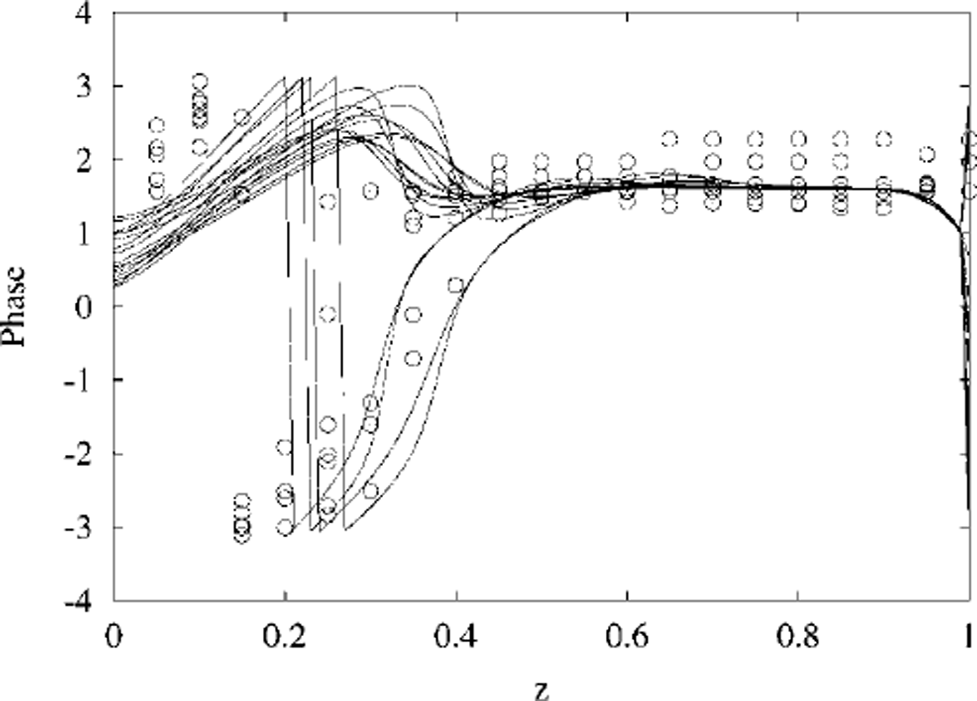
Fig. 11. Predicted and observed values of the phase of temperature oscillations, plotted together for comparison. all of the data have been plotted as circles, and the numerical results as solid lines.
Phase matches between data and numerical model solutions are excellent, at all depths. The jumps that can be seen in the phases are due to restricting phase to principal values between (-π,π).
Amplitudes also match well in the shallow conductive layer, but the deep amplitudes are larger (by a factor of ∼ 10) in the measured data than predicted by the model solutions.
As noted above, deep amplitudes are largest after the ice has warmed. Key factors that might account for the discrepancy are scattering lengths and absorption coefficients. However, previous studies of the temperature dependence of scattering lengths in sea ice (Reference Haines, Buckley and TrodahlHaines and others, 1997) have shown that the deep scattering lengths are not perceptibly changed by warming.
This suggests that the anomalously high temperature-oscillation amplitudes observed at depth may be due to the extra absorption attributable to the presence of algae (Reference Zeebe, Eicken, Robinson, Wolf-Gladrow and DieckmannZeebe and others, 1996) or dissolved organic material in the deeper layer (Reference Perovich, Roesler and PegauPerovich and others, 1998), since the Monte Carlo simulations we conducted assumed that attenuation of photons between scattering centres was due only to pure ice. The discrepancy between data and numerical solution amplitudes at depth shows as a deviation in slope on the semilog plot, suggestive of a distributed effect rather than any localized concentration of algae in strata. Reference GrenfellGrenfell (1991) notes that absorption by algae can reduce transmitted radiation by more than a factor of ten at certain visible wavelengths. Reference Perovich, Roesler and PegauPerovich and others (1998) discuss possible mechanisms that could enhance entrapment of organic matter during the slow growth of congelation ice that typifies the deeper sea-ice layer, and suggest that an alternative ice-growth mechanism such as a sub-ice frazil layer or buoyant anchor ice could bring particles of organic matter to the ice. We would add to this list the possibility of platelet ice also bringing organic matter to be incorporated into the sea-ice matrix (e.g. Reference Crocker and WadhamsCrocker and Wadhams, 1989; Reference Jeffries, Weeks, Shaw and MorrisJeffries and others, 1993; Reference Gow, Ackley, Govoni and WeeksGow and others, 1998; Reference Smith, Langhorne, Trodahl, Haskell, Cole and ShenSmith and others, 1999).
The data presented here represent a direct measurement of the effect of solar radiation penetration in sea ice, and may serve to further inform parametric models of solar heating of sea ice, particularly in light of recent results that emphasize the importance of daily forcing effects (Reference Hanesiak, Barber and FlatoHanesiak and others, 1999). We plan to explore more fully the changes in deep amplitudes and layer thickness as ice temperature changes, in a future publication. We also plan to take advantage of small parameters that appear in the linearization Equation (14) and explore the implications of analytic asymptotic solutions for the oscillatory response of sea-ice temperature to penetrating solar radiation.
Acknowledgement
We are grateful to S. Wilkinson for help with the 1999 data.


