


Introduction
The McMurdo Dry Valleys (MDV), Antarctica, are a polar desert with alpine glaciers, ephemeral streams and perennially ice-covered lakes. The region receives little precipitation (snow), and essentially all water in the lakes and streams originates as glacier melt (Reference FountainFountain and others, 1999). Because summer temperatures hover near and often below the melting point, small variations in the energy balance cause the meltwater flux to vary seasonally by as much as an order of magnitude. The ecosystem in the MDV is extremely sensitive to small changes in climate and the availability of water (Reference DoranDoran and others, 2002a). Meltwater production from the glaciers is therefore important for understanding the stability of the ecosystem in the MDV.
Surface melt on glaciers can be modeled through an energy-balance approach, in which the melt rate is determined by the energy exchange to and from the surface. However, energy-balance models are not applicable when detailed meteorological measurements are unavailable (Reference HockHock, 1999). An alternative approach is to use a temperature-index model, in which melt rate is related to air temperature alone. Temperature-index models perform well because air temperature is a factor in all terms in the energy-balance equation, other than shortwave radiation. Thus, it correlates well with most terms in the energy-balance equation (Reference BraithwaiteBraithwaite, 1981). While temperature-index models are widely used because air temperature data are widely available and easy to interpolate and forecast (Reference HockHock, 2003), they fail to account for spatial variations in melt caused by changes in albedo, net radiation (from topographic effects), wind and humidity (Reference HockHock, 1999). The accuracy of these models decreases with increasing temporal resolution because they fail to account for temporal changes in the above factors (Reference HockHock, 2003). Attempts to improve melt predictions have been based on accounting for temporal changes in some of these factors (e.g. Reference Kustas, Rango and UijlenhoetKustas and others, 1994; Reference Kane, Gieck and HinzmanKane and others, 1997; Reference HockHock, 1999).
Previous work on meltwater modeling in the MDV has utilized both energy-balance (Reference ChinnChinn, 1987; Reference LewisLewis, 1996; Reference Lewis, Fountain and DanaLewis and others, 1998, Reference Lewis, Fountain and Dana1999) and temperature-index models (Reference Clow, McKay, Simmons and WhartonDana and others, 2002; Reference JarosJaros, 2003). The model of Reference Clow, McKay, Simmons and WhartonDana and others (2002) uses satellite-inferred surface temperatures to estimate diurnal and seasonal stream flow. Using 1.1 km resolution pixels, they found a good correlation with the number of pixels with temperature > –14˚C and stream flow. Given the frequent coverage of the valley, Reference Clow, McKay, Simmons and WhartonDana and others (2002) were able to predict flow biweekly. Reference JarosJaros (2003) modeled the spatial variations in meltwater production based on the temperature lapse rate but not the seasonal variation. Reference BombliesBomblies (1998) also examined spatial variations of stream flow based on patterns of solar shading on the glaciers. Here, we take the work of Reference BraithwaiteBomblies (1998) and Reference JarosJaros (2003) a step further and model both spatial and temporal variations in meltwater production. We present three simple models to predict total summer (December–January) meltwater runoff from all of the glaciers contributing to the three major lakes in Taylor Valley. In addition to a basic temperature-index model, we examine a temperature and solar-radiation index model and a model that includes wind speed. Our overall goal is to be able to estimate past variations in surface runoff, over decades to millennia, based on only a few parameters.
Climate and Setting
The MDV are located on the west coast of McMurdo Sound at 77˚00′ S, 162˚52′ E (Fig. 1). They cover an area of approximately 4800 km2, the largest relatively ice-free area in Antarctica (Reference FountainFountain and others, 1999), and contain alpine glaciers, ephemeral streams and perennially ice-covered lakes. Taylor Valley, approximately 36 km long, with an area of about 400 km2, is bounded by the Asgard Range to the north and the Kukri Hills to the south. The mean annual precipitation in the valley bottom is <10cmw.e. (Reference FountainFountain and others, 1999), making the valley a polar desert. Mean annual temperature varies between –14.8 and –23.0˚C (Reference DoranDoran and others, 2002b), with mean summer temperatures of about –2˚C. Monthly average wind speeds range from 2 to 4 ms–1 and tend to increase from the coast inland (Reference FountainFountain and others, 1999; Reference DoranDoran and others, 2002b; Reference Nylen, Fountain and DoranNylen and others, 2004). Katabatic winds flow off the ice sheet and warm adiabatically as they descend into the valley, creating a locally warmer and drier atmosphere (Reference DoranDoran and others, 2002b; Reference Nylen, Fountain and DoranNylen and others, 2004). This favors sublimation and limits the energy available for melt. An up-valley gradient in climate exists with increasing air temperatures, decreasing humidity and higher wind speeds (Reference FountainFountain and others, 1999; Reference DoranDoran and others, 2002b). For 4–10 weeks during the austral summer the glaciers feed more than 24 ephemeral streams that flow across the valley bottom to one of three enclosed lakes (Reference McKnight, Niyogi, Alger, Bomblies, Conovitz and TateMcKnight and others, 1999) (Fig. 1).

Fig. 1. Site map of Taylor Valley, Antarctica, showing locations of glaciers, lakes, stream gauges and meteorological stations.
The glaciers in Taylor Valley are polar alpine and flow from the Asgard Range and the Kukri Hills. The one exception is Taylor Glacier, an outlet of the East Antarctic ice sheet. All of the larger glaciers (e.g. Taylor, Canada and Commonwealth Glaciers) terminate in vertical cliffs. The north-facing glaciers in the Kukri Hills have higher equilibrium-line altitudes (ELAs) than the south-facing glaciers in the Asgard Range, due to differences in solar radiation (Fountain and others, 1999). Because of topography differences, accumulation basins and glaciers are larger in the Asgard Range than in the Kukri Hills. Cool, dry, windy conditions during summer favor sublimation over melt (Reference ChinnChinn, 1987) and account for 40–80% of the ablation on Canada Glacier (Reference Lewis, Fountain and DanaLewis and others, 1998). Melt can occur at air temperatures below 0˚C (Reference ChinnChinn, 1987; Reference Lewis, Fountain and DanaLewis and others, 1998; Reference Fountain, Tranter, Nylen, Lewis and MuellerFountain and others, 2003), some of which occurs in the subsurface through a solid-state greenhouse effect (Reference Fountain, Tranter, Nylen, Lewis and MuellerFountain and others, 2003). Melt has also been observed on cliff faces while little or no melt was observed on the surface (Reference ChinnChinn, 1987). Because of reduced wind speeds, lower albedo and higher incoming longwave radiation, terminus cliffs can contribute up to 20% of the total meltwater runoff (Reference Lewis, Fountain and DanaLewis and others, 1998).
Data
Stream-flow monitoring began in Taylor Valley in the 1990/91 season and has continued (except for the 1992/93 season) through the 2001/02 season. We use data from eight stream gauges in the Fryxell basin, two in the Hoare basin, two in the Bonney basin and one at the coast. There are two additional stream gauges in the Bonney basin on streams draining from Taylor Glacier. Data from these were not used in the correlation of the model because the records are extremely poor (>25% error) as a result of unstable stream channels and sediment load. The data were generally recorded at 15 min intervals. Some sites lack data for the entire 11 year record because of installation date and instrumentation failures. In other cases, the recorded data are not very good due to sedimentation or freezing problems. Stream discharge quality is determined qualitatively by how often the stream gauge was visited during the season, the amount of turbulent flow, and comparisons between inside and outside gauge readings (personal communication from K. Cozzetto, 2004). Good stream-flow measurements are considered accurate to within 10%, whereas poor measurements may be off by >25% (http://huey.colorado.edu/ 2004). Missing stream-flow records were replaced by estimates from Canada Stream flowing from Canada Glacier. In total, only 19 of 143 seasons of record were estimated for the 13 streams. All linear correlations were significant with 95% confidence, and r2 values (the fraction of the observed variance explained by the regression) ranged from 0.77 to 0.97. Preliminary analysis showed that 94% of the runoff from the glaciers occurred during December and January. The 15 min stream discharge data are therefore totaled over December and January and converted from discharge (m3 s–1) to volume (m3).
Eight meteorological stations collect data year-round in Taylor Valley. Four stations are on glaciers and four are on the valley floor. Air temperature is measured every 30 s and averaged every 15 min. Other measurements include wind speed and direction, relative humidity, radiation and ice or soil temperatures. The meteorological station at Lake Hoare, starting in December 1985, contains the longest record (Reference Clow, McKay, Simmons and WhartonClow and others, 1988). Mass-balance measurements have been made on Canada, Commonwealth and Howard Glaciers since the 1993/94 season and on Taylor Glacier since the 1994/95 season. These measurements consist of stake measurements that were taken at the beginning and end of the summer seasons to determine the summer and winter balance. We use the summer balance measurements in the ablation zone to constrain the melt calculation.
Methods
Our approach to estimating total runoff is simple. Runoff from each glacier is based on the total melt and contributing area:
where M is the total seasonal melt (in m) over the fraction of glacier area dA and Q is the total seasonal runoff volume. This equation is approximated by
where seasonal specific melt is a function of seasonal average temperature (Tx,y,z), solar radiation (I) and wind speed (U) (and possibly other factors not accounted for here), which themselves are assumed to be functions of location, and the area of an altitude interval on the glacier, A(z).
Air temperature
The surface air temperatures we use in the models discussed below are seasonal averages (individual observations are recorded at 15 min intervals and vary with standard deviations of 2.1–3.3˚C over each season) adjusted to account for their distance relative to a reference location. The seasonal air temperature within Taylor Valley increases with distance from the coast (Reference DoranDoran and others, 2002b) and from the valley bottom as a result of warming over the exposed soil. Air temperature also decreases with elevation. The spatial variation in summer temperature can be approximated by
(personal communication from C. Delany, 2003), where x is the distance from the coast, y is the distance from the valley bottom and z is the elevation (all in km) and T0 is the average temperature at the coast for the season. The vertical gradient (–9.8˚Ckm–1) is the dry adiabatic lapse rate. The other gradients were determined by a least-squares polynomial fit to the average summer air-temperature measurements across the valleys from the 1997/98 season. Here, we have modified Equation (3) to predict valley temperatures based on the meteorological station at Lake Hoare, which has the longest-running record. The modified form of Equation (3) is
where the subscript H indicates the value at Lake Hoare. This equation was tested against the summer average temperatures from the eight meteorological stations in the valley for all seasons. The residuals are presented in Figure 2. The coefficient of determination between the measured and calculated temperatures was r2 = 0.95. The largest error was 0.83˚C on Commonwealth Glacier.
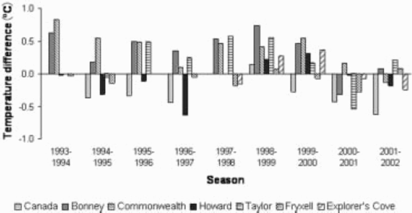
Fig. 2. Residuals between modeled temperature and measured seasonal (December–January) temperature at the Taylor Valley meteorological stations.
Modeling seasonal runoff
To estimate total meltwater contribution to the lakes, we start with the simplest possible temperature-index model M = f (Tx,y,z) (hereafter, T model). Many temperature-index models are based on a linear relationship between temperatures and melt (Reference Kustas, Rango and UijlenhoetKustas and others, 1994; Reference BraithwaiteBraith-waite, 1995; Reference Kane, Gieck and HinzmanKane and others, 1997; Reference HockHock, 1999). Plots of runoff and ablation vs temperature in Taylor Valley clearly show a non-linear relationship, and runoff/ablation increases sharply as temperatures warm above –1.5˚C. A variety of mathematical relations (power, hyperbolic, exponential, etc.) were used to fit seasonal melt with temperature. The overall best fit was given by an exponential of the form

where A, B and E are empirically determined parameters. The constant, E, effectively prevents Equation (5) from calculating melt below a threshold temperature. T∗ is the normalized air temperature, where T̄ x , y, z and ST are the mean and standard deviation of temperatures calculated at multiple points on the glaciers in the valley for all 11 seasons, respectively.
Melt is sensitive to small variations in solar radiation (i.e. incidence of solar radiation) in the polar environment (Reference Lewis, Fountain and DanaLewis and others, 1998, Reference Lewis, Fountain and Dana1999). A new model was developed to include spatial variations in solar radiation as well as temperature (TI model). The potential direct solar radiation, I, is calculated by

(Reference HockHock, 1999), where I0 is the solar constant (1368Wm–2; Reference Fröhlich, McBean and HantelFröhlich, 1993), R is the instantaneous sun–Earth distance, Rm is the mean sun–Earth distance, a is the mean atmospheric clear-sky transmissivity, P is the atmospheric pressure, P0 is the mean atmospheric pressure at sea level, ζ is the zenith angle and θ is the incident angle between the solar ray and the normal to the surface. The incident angle of the solar ray and Earth surface is calculated by
where β is the angle of the surface slope, ζ is the zenith angle, φsun is the solar azimuth and φslope is the aspect of the surface. Slope and aspect are measured on multiple points in the ablation zone of each glacier. The potential solar radiation is calculated at each point for every hour of each day from 1 December to 31 January. The results are averaged over the hours of each day, then over all of the days and finally over all the points on the glacier, yielding a solar radiation index for each glacier (Table 1).
Table 1. Solar radiation and wind speed for glaciers

As with the initial TI model, we choose an exponential relationship of the form

where I∗ is normalized potential direct solar radiation, and Ī and SI the mean and standard deviation of solar radiation calculated from the solar radiation indices of all the glaciers in the valley, respectively.
Our final model (TIU model) also includes variations in wind speed because wind is an important factor in the turbulent transfer of heat exchange with the surface and typically reduces melt in the MDV (Reference Lewis, Fountain and DanaLewis and others, 1998; Reference FountainFountain and others, 1999; Reference JohnstonJohnston, 2004).It is given by the relation

where U* is normalized average wind speed for each glacier in Taylor Valley. The summer average wind speed (U) was calculated by averaging the summer wind speed over all years of record for each meteorological station. The wind regime was estimated by means of an ordinary kriging method in which an ellipse defined the kriging domain for Taylor Valley, and wind speeds were estimated using the nearest two to four meteorological stations (personal communication from C. Delany, 2004) (see Table 1). The mean (Ū) and standard deviation (SU) of the wind speed between all glaciers was calculated from summer average wind speed over all glaciers in the model. In all models (Equations (5–9)) the normalized form of the independent variable is used to assess the relative importance of each variable.
Many of the glaciers in Taylor Valley have vertical cliff faces at their termini and along their lateral edges. Melt from the cliff face can be 15 times that on the glacier surface and is caused by a lack of snow accumulation on the cliff face (which decreases the albedo), increased longwave radiation from the valley floor and lower wind speeds, which reduce sublimation (Reference Lewis, Fountain and DanaLewis and others, 1998, Reference Lewis, Fountain and Dana1999). Melt from a cliff face can contribute up to 20% of the total runoff (Reference Lewis, Fountain and DanaLewis and others, 1998) and therefore cannot be ignored. Attempts were made to incorporate cliff aspect and shading into the models, with little success because of the complexities of the enhanced melt on the cliffs. Instead we calculate cliff melt (Mc) as a separate component that is additive to the melt calculated from the previously defined models
where a = 0.48 m, b = 0.3 and c = –0.026m were determined by the fit to measured ablation on the cliffs of Canada Glacier. We apply this equation to estimate the cliff melt per unit area on all cliffs in the study area. The total volume of cliff melt is then calculated as the product of cliff melt and cliff area. The total melt from the cliffs is then added to the total runoff over the glacier surface (Equation (2)).
Surface melt is also adjusted for evaporation from the streams, which is a function of stream length and width. That is, a relatively longer and wider stream suffers relatively larger losses due to evaporation. Evaporation-pan experiments yield a specific volume rate of 7.14×10⁻⁸ms–1 of water (Reference Gooseff, McKnight, Runkel and VaughnGooseff and others, 2003), which is multiplied by the length of the season (2 months) and the stream length and width to obtain volume loss and is subtracted from the melt volume from the glacier.
Model application
Each glacier in Taylor Valley was divided into sections bounded by the drainage-flow divides, as defined by surface elevation contours (Fig. 3). The sections are further divided by the 50 m elevation contours to account for the reduction of melt with increase in elevation by the temperature lapse rate in Equation (4). The seasonal melt is calculated for the midpoint of each section, using Equations (5), (8) and (9) depending on the model applied, multiplied by the surface area of each section, and summed over the entire drainage or glacier (Equation (2)).

Fig. 3. Canada Glacier divided up by the 50m contours and drainage divides. Temperature and melt are calculated at each point, and melt is then multiplied by the area of the section it occupies.
The coefficients for each model are determined by fitting Equations (5), (˚) and (9) to the measured ablation from Canada, Commonwealth, Howard and Taylor Glaciers using the Marquardt–Levenberg method by means of PSI-PLOT software. Because sublimation makes up a significant proportion of ablation, the ablation data were divided in half before fitting. Runoff was then calculated by Equation
(2) and compared to the measured runoff. Small adjustments were made to coefficients A and B to better fit the measured runoff while not exceeding the measured ablation.
Model accuracy is evaluated using the coefficient of determination, which indicates what fraction of the variability in runoff is accounted for by the model

where Qm and Qc are the measured and calculated runoff for each season respectively and Q̄m is the mean measured runoff over all seasons. Negative r2 values indicate the variability in the difference between measured and calculated runoff is larger than the variability in the measured runoff. The total volume error for all seasons was also calculated by dividing the difference between the sum of calculated and the sum of measured runoff by the sum of measured runoff over all 11 seasons.
Results
Table 2 shows the coefficients of the final models, and Table 3 shows the corresponding r 2 values. Results are presented for representative glaciers in each basin that are drained by streams with the most complete flow records. We present results for individual glaciers to demonstrate how the models perform for glaciers with varying characteristics across the valley. We are most concerned with being able to estimate the total meltwater input into each lake, so we also present results for each basin. For individual glaciers, as identified in Table 3, the discharge used in calculating r 2 is the sum of all streams flowing from that glacier, and for the basins the discharge is the sum of all the streams flowing into the lake. Note that Taylor Glacier is not included because the runoff measurements from the streams draining the glacier are generally poor and were not used in the correlation. Many other glaciers are also not included because they lack stream data. Within the Lake Fryxell basin, the T model predicted the summer runoff from the south-facing Canada and Commonwealth Glaciers (r2 = 0.69 and 0.67 respectively) well and the north-facing glaciers poorly (Fig. 4; Table 3). The total runoff for all seasons is underestimated by 29% in the Fryxell basin and by 1% in the Hoare basin. In the Bonney basin the runoff did not match particularly well (63% underestimate of total runoff), with runoff from Rhone Glacier being severely underestimated. The T model could have fit any one of these glaciers given the appropriate coefficients. However, we want one model with one set of coefficients so that we can make a reasonable estimate for runoff from the glaciers in Taylor Valley that have no records of runoff. Results from the TI model were better for the north-facing glaciers in the Fryxell basin and did not change the results for the south-facing glaciers. The sun is higher in the northern sky (36° above horizontal) than in the southern sky (10.5˚), resulting in a significant difference in insolation between the north-and south-facing glaciers (roughly 285 and 250Wm–2, respectively). The total runoff for all seasons using the TI model is only underestimated by 15% in the Lake Fryxell basin. In the Lake Hoare basin, the model predicts runoff from Canada Glacier well, but the overall results for the Hoare basin are poor (49% underestimate of total runoff) due in part to under-predicted runoff from Suess Glacier located at the western edge of Lake Hoare. Most of the runoff into Lake Hoare comes directly from Canada Glacier, so the real effect of the under-prediction for Suess would be smaller. In the Bonney basin, the melt rate from Taylor Glacier is severely over-predicted (Fig. 5) and the runoff for Rhone Glacier is under-predicted (Fig. 4d). To some degree these errors cancel, but Taylor Glacier is a much larger glacier and potentially has much greater influence on the basin runoff when the temperatures are warm.

Fig. 4. Calculated and measured runoff for Canada Glacier (a), Commonwealth Glacier (b), Howard Glacier (c) and Rhone Glacier (d). (a, b) The models perform well for Canada and Commonwealth Glaciers. (c) The TI and TIU models estimate runoff for Howard Glacier well, but the T model underestimates runoff during the warmer seasons. (d) All three models underestimate runoff for Rhone Glacier, with the TI and TIU models performing the worst.
Table 2. Model coefficients for the temperature index model (T), the temperature–insolation model (TI) and the temperature–insolation–wind-speed model (TIU)

Table 3. Coefficients of determination and total volume error for the temperature index model (T), the temperature–insolation model (TI) and the temperature–insolation–wind-speed model (TIU)


Fig. 5. Taylor Glacier calculated and measured melt (measured melt is assumed to be half of the measured ablation). Summer average temperatures are calculated at each stake on the glacier surface from Equation (4) for direct comparison.
To improve the melt-rate prediction on Taylor Glacier, we included wind speed in the melt equation. The Bonney basin in general, and Taylor Glacier in particular, is windier than the glaciers in the Fryxell basin. Summer average wind speed on Taylor and Canada Glaciers is 4.5 and 3.2 ms–1, respectively. As previously mentioned, wind plays an important role in the energy balance of the ice surfaces. For air temperatures below freezing, higher winds increase sublimation and cool the surface through latent- and sensible-heat exchange, compensating for the heat gain from solar radiation and eliminating melt. Results from the TIU model showed that the predicted melt from Taylor Glacier is still poor and the predicted runoff for the Bonney basin, the motivation for the model, decreased significantly. The total volume of runoff in the Bonney basin is now underestimated by 84%. Unfortunately, we cannot examine the mismatch in any detail because of the poor runoff measurements from the streams draining Taylor Glacier. The effect of including wind improved the results for the Lake Hoare basin while only slightly changing the results for the Fryxell basin (Table 3). In general, the models are more sensitive at warmer seasonal average temperatures.
A change in seasonal average temperature from –5˚C to – 4˚C increases the modeled runoff for Canada Glacier by about 104m3 for the three models. However, a change in average temperature from –1˚C to 0˚C results in an increase of modeled runoff by about 106m3 for Canada Glacier. Not only is runoff sensitive to small changes in temperature at warmer temperatures, but the addition of the solar and wind terms also influences the calculated runoff most at warmer temperatures.
Overall, the best results are from the TI model in the Fryxell basin with a coefficient of determination of r2 = 0.73. The model overestimates runoff from Crescent Glacier and underestimates runoff from Von Guerard Glacier, resulting in low r2 values (Table 3). All three models consistently under-predict stream flow for the two streams in the Bonney basin that flow from Rhone, LaCroix, Sollas and Marr West Glaciers. The south-facing glaciers in the Bonney basin (Rhone and LaCroix) are characterized by steep rough surfaces with narrow termini. These glaciers receive no direct solar radiation when the sun is in the north, and thus have low average solar radiation (Table 1). The rough surfaces on these glaciers probably reduce wind speed over the surface, reducing the turbulent exchange terms of latent and sensible heat, leaving more energy available for melt (Reference Lewis, Fountain and DanaLewis and others, 1999). Similarly, the runoff from Suess Glacier at the west end of Lake Hoare is under-predicted from the TI model (not shown). This side of the glacier is characterized by many vertical faces with rock debris spread over the surface. The vertical faces, lower albedo caused by the rock, and slower wind speeds probably enhance melt on this glacier. A more detailed study of the melt production on these glaciers is needed to understand the factors controlling their melt.
Discussion and Conclusions
The temperature-index model made reasonable predictions of runoff in Taylor Valley, performing best in the Fryxell basin. Incorporating spatial differences in solar radiation resulted in the best overall model. The addition of wind speed improved the results for the Lake Hoare basin, but gave significantly worse results for the Bonney basin. The intent of including the wind speed was to improve the results specifically for the Bonney basin. Unfortunately, because of the lack of usable runoff records for Taylor Glacier, we cannot determine how well the models predict runoff for Taylor, which is the largest contributor to the Bonney basin. Two glaciers within the basin, Rhone and LaCroix, are steep glaciers with extremely rough surfaces probably resulting from avalanched rock debris (Reference JohnstonJohnston, 2004), which enhances the melt component of ablation. We observe a similar process on Suess Glacier at the west end of Lake Hoare. Our models currently do not account for these factors, and underestimate their runoff. However, we plan to pursue this problem in the future. The variations in melt between glaciers, due to differences in surface morphology, underscore the conclusions from other authors (Reference Lewis, Fountain and DanaLewis and others, 1999; Reference Johnston, Fountain and NylenJohnston and others, 2005) that small changes in surface slope and in wind speed can result in large changes in melt production. Overall, the exponential increase in melt runoff as air temperatures warm to near-melting temperatures reflects this sensitivity. Our melt runoff models capture this behavior, and, while some differences exist between glaciers, the results are reasonable and will be useful for estimating past hydrological conditions in the valleys.
Acknowledgements
The authors thank C. Delany for his help with GIS and the temperature equation, and the reviewers J. Staiger, S. Price and B. Vaughn for their suggestions which clarified the paper. Funding for this work came from the US National Science Foundation, Office of Polar Programs NSF OPP 0096250.


