Regional atmospheric climate model

We use the output of the high-resolution (~5.5 km horizontal gridding) regional atmospheric climate model RACMO2, version 2.3 (Reference LenaertsLenaerts and others, 2014; Reference Van Wessem, Reijmer, Lenaerts, Van de Berg, Van den Broeke and Van MeijgaardVan Wessem and others, 2014), with its spatial domain focused on DML (~25° W to ~35° E) (Fig. 1). RACMO2 has been used before to map Antarctic SMB at a lower horizontal resolution (~27 km; Reference Lenaerts, Van den Broeke, Van de Berg, Van Meijgaard and MunnekeLenaerts and others, 2012a), but that resolution is insufficient to properly resolve the topography of an average-sized ice rise.

Fig. 1. RACMO2 topography inside the model domain (Reference Bamber, Gomez-Dans and GriggsBamber and others, 2009), with 100 m vertical spacing from 0 to 1000 m a.s.l. and 500 m spacing from 1000 to 4000 m a.s.l. Blue represents the ocean, grey the ice shelf and white the grounded ice. The red crosses indicate locations of ice rises. The green box shows the extent of the maps presented in Figures 3, 5a and 7. The red box in the inset map shows the location of the domain on Antarctica. Locations discussed in the paper are indicated on the map.

RACMO2 is forced at its lateral boundaries by atmospheric profiles of the ERA-Interim reanalysis from the European Centre for Medium-range Weather Forecasts (ECMWF 2001–12; Reference Dee and UppalaDee and Uppala, 2009), and is free to evolve in its inner spatial domain. The relaxation zone, where the ERA-Interim fields are downscaled to RACMO2 resolution, is sufficiently wide (32 RACMO2 gridpoints, i.e. ~180 km) and located over the ocean where possible. Sea-surface temperature and sea-ice extent in RACMO2 are also prescribed by the ERA-Interim analysis. The snow model that is interactively coupled with RACMO2 includes physical descriptions and temporal evolution of snowmelting, percolation and runoff (Reference Ettema, Van den Broeke, Van Meijgaard, Van de Berg, Box and SteffenEttema and others, 2010), snow albedo (Reference Kuipers Munneke, Van den Broeke, Lenaerts, Flanner, Gardner and Van de BergKuipers Munneke and others, 2011) and drifting snow (Reference LenaertsLenaerts and others, 2012b). The snowpack is initialized with data from a previous RACMO2 simulation (Reference Lenaerts, Van den Broeke, Van de Berg, Van Meijgaard and MunnekeLenaerts and others, 2012a).

Elevation model

In this study, we use the digital elevation model (DEM) provided by Reference Bamber, Gomez-Dans and GriggsBamber and others (2009), which has been compiled from satellite-based laser and radar altimetry from the Ice, Cloud and land Elevation Satellite (ICESat) and European Remote-sensing Satellite (ERS), respectively. It covers the entire Antarctic continent and is gridded to 1 km postings. The ice rises in our sector of interest appear clearly in the DEM, even after regridding this DEM to the RACMO2 horizontal resolution (5.5 km; Fig. 1). However, ice rises have relatively steep surface slopes, which introduces errors into the DEM, since the altimeter reflections do not originate from the sub-satellite points. This may result in locally large elevation errors (e.g. Reference Drews, Rack, Wesche and HelmDrews and others, 2009; Reference Wesche, Riedel and SteinhageWesche and others, 2009). In the future, such problems will be overcome, for example, by using the interferometric capabilities of CryoSat-II (Reference Helm, Humbert and MillerHelm and others, 2014). In this study, however, we decide to use the DEM of Reference Bamber, Gomez-Dans and GriggsBamber and others (2009), because it provides a spatially continuous and consistent dataset. We keep in mind that errors in the applied elevation model will propagate to simulated absolute SMB values; however, we expect that the simulated SMB gradients will not alter dramatically with an improved DEM.

Meteorological data

To evaluate the temperature, precipitation and SMB simulated by RACMO2, we use data from three weather stations (Fig. 1). The permanently manned station, Neumayer III, is located on the flat Ekström Ice Shelf, ~20 km from the ice-shelf edge, and has provided quality-controlled, detailed meteorological observations since 1983. We use daily averaged data covering the period January 2011–December 2011 (König-Langlo, 2011). We also use daily averaged data for 2011 from an automatic weather station (AWS11; Reference Van den Broeke, Van As, Reijmer and Van de WalVan den Broeke and others, 2004) installed on the ridge of Halvfarryggen, an ice promontory located ~120 km southeast of Neumayer III (~700 m a.s.l.; Reference Drews, Martín, Steinhage and EisenDrews and others, 2013; Reference Van Wessem, Reijmer, Lenaerts, Van de Berg, Van den Broeke and Van MeijgaardVan Wessem and others, 2014). Finally, we use measurements of snowfall and snow height (2009–12) and snowfall rate (2011–12) available from the Princess Elisabeth base (PE base; Fig. 1). PE base is located on Utsteinen ridge (1390 m a.s.l.; 72° S, 23° E) just north of the Sør Rondane mountains in the escarpment area of eastern DML, ~200 km southwest of the ice-shelf edge. The snow height was measured by a sonic height ranger installed as part of AWS16, located in a valley 300 m east of PE base; annual SMB was inferred using an annual mean snow density measured on site (Reference Gorodetskaya, Van Lipzig, Van den Broeke, Mangold, Boot and ReijmerGorodetskaya and others, 2013). Snowfall rate is derived from a micro rain radar 2 (MRR) vertically profiling 24 GHz radar installed at PE (Reference GorodetskayaGorodetskaya and others, 2014a), hereafter referred to as snow radar. Here we use daily total snowfall rates, S, estimated based on the near-surface radar reflectivity, Ze. Uncertainty in snowfall rate estimates depending on snow-particle microphysical properties is considered by applying a range of Ze/S relationships for dry snow (Reference MatrosovMatrosov, 2007). Although PE base is not located on or near an ice rise, it retrieves the only direct measurements of snowfall in DML.

Snow stakes and firn cores

Along with the model evaluation using meteorological data, we compare the RACMO2 SMB with local SMB estimates derived from a combination of snow-stake and firn-core measurements. In January 2012, we placed a network of 73 aluminium stakes on Kupol Ciolkovskogo and 79 stakes on Kupol Moskovskij (Fig. 1) as part of a GPS occupation campaign. We placed 3 m long aluminium stakes ~1 m into the snow surface, measured the initial height of each stake from the snow surface, and reoccupied the measurement 1 year later. To ensure that the aluminium stakes were well anchored, they were manually driven into the snow to a hard layer at ~1 m depth. We assume that the magnitude of firn compaction is much smaller than the measured stake height difference related to SMB. We believe that this is a valid assumption in this case, since we are solely interested in the SMB pattern over the ice rises, rather than the absolute value of the single-year SMB values.

In order to determine the local SMB from the stake snow heights, we collected 3 m firn cores at six locations on Kupol Ciolkovskogo and 14 locations on Kupol Moskovskij in January 2013. We measured the length, diameter and mass of each core section. The cumulative length of the measured core sections does not correspond to the relative stake height differences at the locations; to estimate the density of the surface layer, we calculate the weighted mean density of multiple core sections to the depth of the accumulated snow. To estimate the error due to horizontal variability in near-surface density (the cores and the stakes are < 5 m apart), we drilled two separate cores close to one another. The resulting SMB error is assumed equal to three times the observed SMB difference between the cores, i.e. 15 mm w.e. a^-1.

Ground-penetrating radar

Ground-penetrating radar (GPR) is a standard method to spatially extrapolate accumulation measurements from firn cores (e.g. Reference Spikes, Hamilton, Arcone, Kaspari and MayewskiSpikes and others, 2004; Reference EisenEisen and others, 2008). The underlying principle assumes that shallow, laterally continuous internal-reflection horizons in the radar data are isochrones that are not deformed significantly by ice dynamics (shallow-layer approximation; Reference Waddington, Neumann, Koutnik, Marshall and MorseWaddington and others, 2007). For data regarding Halvfarryggen and Derwael Ice Rise, only one firn core was available, which necessitates the additional assumption that the depth/density profile does not change laterally.

The radar profile on Derwael Ice Rise presented in Figure 2 was collected in 2012 and spatially extended by ~10 km towards the southeast in 2013. It was acquired using a commercial 400 MHz antenna. For the travel-time to depth conversion, we use a velocity/density model based on the mixing formula given by Reference LooyengaLooyenga (1965). The density/depth scale stems from a combination of discrete firn-core samples (Reference HubbardHubbard and others, 2013) and a semi-empirical firn-compaction model (Reference Arthern, Vaughan, Rankin, Mulvaney and ThomasArthern and others, 2010). For the latter, we assume steady state, with a surface subsidence rate equal to the SMB divided by the measured surface density, 400 kg m^-3, and a surface temperature of –15°C. Both values are derived from the firn core drilled on the Derwael Ice Rise divide (Reference HubbardHubbard and others, 2013). The model is vertically integrated until ice density (917 kg m^-3) is reached. We minimize the difference to the core samples by adjusting the activation energy for grain growth to E _g = 41 kJ mol^-1, which closely matches the values given by Reference Cuffey and PatersonCuffey and Paterson (2010).

Fig. 2. GPR profile along Derwael Ice Rise. Note that the transect runs from the upwind slope (S) to the downwind slope (F), i.e. from east to west. The red curve denotes the selected reflector for the SMB estimation. The dashed black line is the position of the ridge and the firn core (Reference HubbardHubbard and others, 2013). The blue line denotes the separation between the data obtained in 2012 and in 2013.

After the travel-time to depth conversion, a single internal-reflection horizon was dated using the annual variability in stable isotopes (δ¹⁸O) measured in the firn core. Near the core site, the internal-reflection horizon is at 22 m depth and the corresponding age is 21 years before 2012. We pick the same isochrone in both datasets, using the characteristic pattern of internal-reflector packages, which is consistent in both datasets. Therefore the radar-derived SMB is a 21 year average for data collected in 2012 and a 22 year average for data collected in 2013. The relative depth of the reflection horizon varies on either side of the divide, which results in the SMB gradient depicted in Figure 2. However, the absolute values derived here are associated with a number of uncertainties: the error of the tentative age/depth scale is ±1 year; the root-mean-square error between the density/depth model and the firn-core data is ±18 kg m^-3, which results in an additional uncertainty of 0.5 m in the conversion from travel time to depth. At the core site, the combined effect of the errors of age/depth scale and of the travel-time to depth conversion on the SMB is ~8% (i.e. ~40 mm w.e. a^-1). We assume this error to be constant along the profile, since the age/depth estimate, which is vertically constant, involves the largest uncertainty. As the observed SMB gradient across Derwael Ice Rise greatly exceeds the associated error, we are confident that the pattern observed is realistic. Additional uncertainties, such as discontinuities between the 2012 and 2013 data, as well as the spatial separation between the radar profile and the core site (~400 m at the closest approach), are constant along the profile, which enhances robustness in the observed spatial gradient.

Temporal variability

DML is a region characterized by a strong interannual variability of SMB (Reference Reijmer and Van den BroekeReijmer and Van den Broeke, 2001; Reference Schlosser, Manning, Powers, Duda, Birnbaum and FujitaSchlosser and others, 2010; Reference Lenaerts, Van Meijgaard, Van den Broeke, Ligtenberg, Horwath and IsakssonLenaerts and others, 2013). Therefore, it is questionable whether 2001–12 is a representative period for the longer-term mean climate. However, when analysing the Antarctic-wide, long-term (1979–2013) RACMO2 simulation (27 km horizontal resolution; Reference Van Wessem, Reijmer, Lenaerts, Van de Berg, Van den Broeke and Van MeijgaardVan Wessem and others, 2014), the 2001–12 DML ice-shelf SMB (331 mm w.e. a^-1) does not differ significantly from the 1979–2013 value (324 ± 48 mm w.e. a^-1 (mean ± standard deviation)). Hence, it is justified to present 2001–12 mean RACMO2 results as a reliable proxy for the long-term, multi-decadal DML climate.

Near-surface climate

Figure 3 presents the simulated mean near-surface climate. Over the ice shelves, near-surface temperature is low (~254 K) and relative humidity high (~90%). They remain nearly uniform over the ice shelves, whereas higher temperatures and lower relative humidities are found over the lower escarpment region connecting the Antarctic plateau with the ice shelves, but also on the ice rises.

Fig. 3. Simulated annual mean (2001–12) near-surface climate in the region 10° W–10° E. (a) 2 m temperature (K). (b) 2 m relative humidity (with respect to ice; unitless). (c) 10 m scalar wind speed (colours) and direction (arrows). (d) Snow density of the top 5 cm (kg m> 3). The locations of Neumayer III (N) and AWS11 (A) (Fig. 4) are shown in (a).

This is further illustrated by comparing daily mean temperature at two neighbouring weather stations (Fig. 4), Neu-mayer III and AWS11, the latter located ~650 m higher than Neumayer III. The difference in elevation results in higher temperatures at Neumayer III in summer (3–4 K), when the surface-based temperature inversion is rather weak. In winter, however, we see prolonged periods with comparable or even higher near-surface temperatures at AWS11. This mainly occurs during periods when the temperature at Neumayer III is very low (< 245 K), i.e. when a strong temperature inversion sets up above the ice-shelf surface, and the temperatures at AWS11 can be 5–10 K higher than at Neumayer III. In 2011, the annual mean temperature was observed to be 256.8 K at Neumayer III and 255.9 K at AWS11, i.e. only a small (0.9 K) temperature difference between an ice shelf and an ice-rise weather station, despite a significant elevation difference (~650 m). RACMO2 simulates this behaviour relatively well, but, despite a correct representation of the elevation difference between Neu-mayer III and AWS11, it overestimates the effect: the annual mean temperature at Neumayer III is underestimated by 1.4 K (255.4 K), with frequent large underestimations in winter (Fig. 4), but RACMO2 agrees with the observed AWS11 temperature within 0.1 K (256.0 K).

Fig. 4. Ten-day running mean, 2 m temperature observed (solid) and modelled (dotted) at Neumayer III (red) and AWS11 (blue). Horizontal bars show the annual mean observed values. The bottom panel shows deviation of the modelled values from the observed values (RACMO2 – observations). Horizontal bars show the annual mean deviations at these two sites. (Fig. 3 shows the locations of these sites.)

We argue that higher temperatures found over ice rises during cold periods are explained by two processes. Firstly, the ice rises are exposed to warmer surrounding air, because of the presence of a semi-permanent surface-based temperature inversion over the ice shelves (Connolley, 1996). Secondly, enhanced vertical mixing in the atmospheric surface layer in winter enhances the downward entrainment of warmer and drier air and partly breaks down the strong stably stratified atmosphere near the surface, which is supported by higher horizontal wind speeds over the ice rises (Fig. 3c), enhancing downward sensible heat flux. This implies that enhanced entrainment, through mechanical turbulence and exposure to warmer ambient air when a strong inversion forms over the surrounding ice shelf, is able to significantly raise near-surface temperatures of ice rises in winter.

Surface mass balance

Simulated mean (2001–12) SMB from RACMO2 in DML is displayed in Figure 5a. Simulated SMB on the ice shelves surrounding the ice rises is relatively homogeneously distributed (200–400 mm w.e. a^-1), but strong spatial SMB variations are found in the vicinity of all ice rises. Annual mean SMB values >1000 mm w.e. a^-1 are modelled on the northeastern (upwind) side of most topographic features, and a clear SMB minimum on the southwestern (downwind) sides. SMB of >2000 mm w.e. a^-1 are simulated on some upwind slopes in western DML (e.g. east of Halvfarryggen).

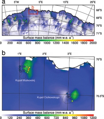
Fig. 5. RACMO2 mean (2001–12) annual SMB in (a) entire coastal DML; zoomed in (b) on Kupol Ciolkovskogo and Kupol Moskovskij (0–4° E). The red box in (a) displays the location of (b). SMB values estimated using firn-core derived densities and stake heights are shown with circles. Contours show the surface topography (Reference Bamber, Gomez-Dans and GriggsBamber and others, 2009) with a resolution of 200 m in (a) and 100 m in (b).

The 2012 DML ice shelves SMB in RACMO2 is insignificantly (< 5%) different from the 2001–12 mean (Reference Van Wessem, Reijmer, Lenaerts, Van de Berg, Van den Broeke and Van MeijgaardVan Wessem and others, 2014), which allows evaluation of RACMO2 SMB in more detail using single-year (2012) measurements around Kupol Ciolkovskogo and Kupol Moskovskij, located ~1–3° E (Fig. 1). On Kupol Ciolkovskogo, our measurements reveal that 2012 SMB ranges between 225 ± 15 and 734 ± 15 mm w.e. a^-1 from the summit to the lowest-elevation site on the upwind side of the ice rise. On the downwind side of the ice rise, the observed SMB ranges from 225 ± 15 to 428 ± 15 mm w.e. a^-1. On Kupol Moskovskij, our 14 SMB measurements show that the single-year SMB ranges between 302 ± 15 mm w.e. a^-1 at the summit and 986 ± 15 mm w.e. a^-1 at the lowest-elevation sites on the upwind side of the ice rise. Together, these measurements constitute a spatially consistent single-year SMB pattern over ice rises, with highest SMB occurring at the low elevation on the upwind side of the ice rises.

Figure 5b compares these local SMB measurements with the mean SMB from RACMO2. We find RACMO2 SMB values of 1000 and 700 mm w.e. a^-1 on the northeastern side of Kupol Ciolkovskogo and Kupol Moskovskij, respectively, whereas a significant SMB minimum is found west of the ice rises, mainly in the case of Kupol Ciolkovskogo (<100 mm w.e. a^-1). Although we have no evidence of this large SMB span from our observations, we find that the RACMO2 SMB compares relatively well with the in situ SMB observations, especially for Kupol Ciolkovskogo; in the case of Kupol Moskovskij, the location of the SMB maximum in RACMO2 is somewhat displaced to the west, which is probably influenced by a poor representation of the ice rise in the DEM. The DEM shows a small ice dome east of Kupol Moskovskij, which does not correspond to our observations.

To understand this simulated SMB variability and compare it with observations in more detail, we zoom in further on the region around Derwael Ice Rise. Figure 6a shows the simulated SMB and the location of the GPR transect across the ice rise, which is parallel to the prevailing near-surface wind direction. The elevation of this transect, measured by kinematic GPS, is shown in Figure 6b. The elevation in RACMO2 (derived from Reference Bamber, Gomez-Dans and GriggsBamber and others, 2009) compares well with the observed elevation, despite an underestimation (~50 m) of the elevation of the divide. This allows for comparison between the observed and simulated SMB along the same transect in Figure 6c. The GPR-estimated SMB shows a gradual increase from 350 ± 40 to 750 ± 40 mm w.e. a^-1 east of the divide; the maximum SMB is located ~15 km east of the divide. From there, SMB sharply decreases in a northwesterly direction. RACMO2 captures the SMB variability reasonably well, although the SMB maximum is displaced to the west by ~5 km. Possible reasons for the discrepancies between model and observations, apart from the inherent model uncertainty and erroneous topography of Derwael Ice Rise in RACMO2 (Fig. 6b), can be ascribed to (1) the assumption of a constant surface snow density in the conversion process from measured two-way travel time of the GPR reflection horizons to SMB and (2) false tracking of reflection horizons in the GPR.

Fig. 6. (a) RACMO2 mean (2001–12) annual SMB around Derwael Ice Rise and location of transect. (b) Elevation profile and (c) mean SMB along the transect according to RACMO2 (black) and derived from the GPR observations (grey; Fig. 2). RACMO2 precipitation, PR, is shown in blue in (c). The vertical dotted line in (b, c) shows the location of the divide. The crosses and numbers in (a) correspond to the distance from the ice ridge, equivalent to the x –axis in (b, c).

Next, we analyse which processes determine this significant spatial variability in SMB. Figure 7 shows the individual simulated SMB components. Precipitation clearly dominates the SMB variability, with large values on the northeastern flanks of the topographic features. This signal is primarily driven by orographic lifting of the relatively humid air that originates from the Southern Ocean. These synoptic precipitation events typically occur only a few (0–5) times per year at irregular intervals, and are related to an atmospheric net southward transport of (sub)tropical moisture (Reference Noone, Turner and MulvaneyNoone and others, 1999; Reference Reijmer and Van den BroekeReijmer and Van den Broeke, 2001; Reference Schlosser, Manning, Powers, Duda, Birnbaum and FujitaSchlosser and others, 2010; Reference Lenaerts, Van Meijgaard, Van den Broeke, Ligtenberg, Horwath and IsakssonLenaerts and others, 2013), sometimes organized in plumes or ‘atmospheric rivers’ (Reference Gorodetskaya, Tsukernik, Claes, Ralph, Neff and Van LipzigGorodetskaya and others, 2014b). This moist air is transported in a southwesterly direction over the flat sea ice and ice shelf, until the flow encounters an ice rise or promontory, leading to locally enhanced precipitation. Note that the direction of moisture flux, driven by synoptic forcing, is northeasterly, and therefore diverges from the mean wind direction (Fig. 3), the latter typically directed from the east to southeast. On the southwestern side of the ice rise, the atmospheric air column has lost part of its moisture, resulting in a precipitation shadow, where precipitation is an estimated factor of 3–10 lower than on the northeastern sides (Fig. 7a).

Fig. 7. RACMO2 mean (2001–12) annual SMB components: (a) precipitation; (b) surface sublimation; (c) drifting snow erosion; (d) drifting snow sublimation. Topography is shown in black contours with a resolution of 100 m.

Such a strong but short-lived character of DML precipitation events is evident from the SMB and snowfall record at PE base from 2009 to 2012 (Fig. 8). The years 2009 and 2011 were characterized by several large accumulation events (Reference Lenaerts, Van Meijgaard, Van den Broeke, Ligtenberg, Horwath and IsakssonLenaerts and others, 2013; Reference Gorodetskaya, Tsukernik, Claes, Ralph, Neff and Van LipzigGorodetskaya and others, 2014b), whereas 2010 and 2012 had no such events. The timing of the two large accumulation events for which snowfall radar data are available (events 1 and 2 in Fig. 8) is very well captured by RACMO2. The model appears to simulate the amount of snowfall well during such events, with RACMO2 indicating 43 mm w.e. of snowfall during event 1 (36 ± 8 mm w.e. according to the radar, depending on the choice of the Ze/S relationship) and 91 mm w.e. during event 2 (69 ± 16 mm w.e. for the snowfall radar).

Fig. 8. Cumulative SMB for 2009–12 at PE base according to RACMO2 (blue) and the observations (red). RACMO2 SMB components are depicted with the dashed line (PR), dotted line (total sublimation) and dash–dotted line (snow erosion). The green lines show the MRR-derived daily snowfall (right axis). Note that the MRR was offline for prolonged periods before and during 2011, shown by the horizontal green dots. ‘1’ and ‘2’ denote snowfall events 1 (14–18 February) and 2 (13–20 December 2011).

RACMO2 suggests higher SMB at PE than the observations, because the model underestimates surface lowering directly following strong snowfall events (Fig. 8); this is probably related to snow compaction (which cannot be corrected for in the observed accumulation record in the absence of continuous surface snow measurements) and/or to the model underestimating local snow erosion after accumulation events. The observed SMB was largest in 2009 (230 mm w.e.), followed by 2011 (227 mm w.e.). In contrast, 2010 (23 mm w.e.) and 2012 (52 mm w.e.) were much drier years. This is also simulated in RACMO2, with high SMB in 2011 (297 mm w.e.) and 2009 (225 mm w.e.), and much lower SMB in 2010 (69 mm w.e.) and 2012 (106 mm w.e.). The model output underscores the significant interannual variability of SMB in DML.

Apart from precipitation, RACMO2 suggests that drifting snow processes are also important for the ice-rise SMB (Figs 7c and d). Snow erosion (20–100 mm w.e. a^-1) occurs just alee of ice-rise ridges, where near-surface winds pick up; the eroded snow is deposited (i.e. negative ER_ds) further down the ice rise, where winds slow down again (Fig. 7c). Drifting snow sublimation is largest (50–200 mm w.e. a^-1) in the windy and dry ice-shelf areas leeward of the ice rises. Unlike drifting snow processes, surface sublimation is small around ice rises (< 20 mm w.e. a^-1; Fig. 7b). Although the individual SMB components cannot be quantified, higher observed surface snow densities, the visual evidence of the presence of many more sastrugi, and larger surface snow grains in satellite products (Reference Scambos, Haran, Fahnestock, Painter and BohlanderScambos and others, 2007) confirm that snow erosion is significant on downwind slopes of Antarctic ice rises. Drifting snow sublimation, and drifting snow erosion even more so, show strong spatial variability, not only on the regional scale, which is resolved by RACMO2 (Fig. 7b and c), but also on much finer, subkilometre scales, related to small undulations in surface topography and wind field. This is especially true in low-precipitation regions, such as on the lee side of ice rises (Fig. 5). In light of the realistic simulation of snowfall by RACMO2 (Fig. 8), it is likely that small-scale drifting snow phenomena, which are not resolved by RACMO2, may explain, at least partly, the discrepancy between model and observations.