Critical earthquake response of elastic–plastic structures under near-fault ground motions (Part 2: Forward-directivity input)
 Kotaro Kojima
 Izuru Takewaki
- Department of Architecture and Architectural Engineering, Graduate School of Engineering, Kyoto University, Kyoto, Japan
The triple impulse input is used as a simplified version of the forward-directivity near-fault ground motion and a closed-form solution of the elastic–plastic response of a structure by this triple input is obtained. It is noteworthy that only the free-vibration appears under such triple impulse input. An almost critical excitation is defined and its response is derived. The energy approach plays an important role in the derivation of the closed-form solution of a complicated elastic–plastic response. It is shown that the maximum inelastic deformation can occur after the second impulse or the third impulse depending on the input level. The validity and accuracy of the proposed theory are discussed through the comparison with the response analysis result to the corresponding three wavelets of sinusoidal waves as a representative of the forward-directivity near-fault ground motion.
Introduction
The near-fault ground motions have been investigated from various viewpoints (Bertero et al., 1978; Hall et al., 1995; Sasani and Bertero, 2000; Alavi and Krawinkler, 2004; Mavroeidis et al., 2004; Kalkan and Kunnath, 2006, 2007; Xu et al., 2007; Rupakhety and Sigbjörnsson, 2011; Yamamoto et al., 2011; Khaloo et al., 2015; Kojima and Takewaki, 2015b; Vafaei and Eskandari, 2015). Those ground motions are characterized by the well-known phenomena called fling-step and forward-directivity (Mavroeidis and Papageorgiou, 2003; Bray and Rodriguez-Marek, 2004; Kalkan and Kunnath, 2006; Mukhopadhyay and Gupta, 2013a,b; Zhai et al., 2013; Hayden et al., 2014; Yang and Zhou, 2014; Kojima and Takewaki, 2015b).
As pointed out in the previous paper (Kojima and Takewaki, 2015b), the fling-step input is a fault-parallel input and the forward-directivity input are a fault-normal input. Those ground motions have been characterized by two or three wavelets and it is recognized that the forward-directivity input has larger effects on structures in general. Recently, some important research works have been conducted. Mavroeidis and Papageorgiou (2003) summarized the characteristics of this class of ground motions in detail and proposed some simple wavelet models (for example, Gabor wavelet and Berlage wavelet). Xu et al. (2007) employed the Berlage wavelet and applied it to the performance evaluation of passive energy dissipation systems. Takewaki and Tsujimoto (2011) used the Xu’s model and proposed a method for scaling ground motions from the viewpoints of drift and input energy demand. Takewaki et al. (2012) employed a sinusoidal wave for pulse-type waves. Kojima and Takewaki (2015b) introduced a simplified input model called “double impulse” (Kojima et al., 2015a) and derived a closed-form solution of the critical elastic–plastic deformation of a single-degree-of-freedom (SDOF) model to the double impulse input. They clarified that (i) a closed-form solution of the critical elastic–plastic deformation can be derived based on a simple energy approach and (ii) the double impulse can be a good substitute of the fling-step input (one-cycle sinusoidal input) under the equivalence assumption of the maximum Fourier amplitude of accelerations. In this paper, the approach by Kojima and Takewaki (2015b) is extended to the forward-directivity input and the intrinsic response characteristics by the forward-directivity are captured.
Most of the previous works on the near-fault ground motions deal with the elastic response because the number of parameters (e.g., duration and amplitude of pulse, ratio of pulse frequency to structure natural frequency, change of equivalent natural frequency for the increased input level) to be considered is tremendous and the computation of elastic–plastic response itself is quite complicated.
In order to tackle such important but complicated problem, a simple input as the double impulse has been employed as a substitute of the fling-step near-fault ground motion in the previous paper (Kojima and Takewaki, 2015b) and a closed-form solution of the critical elastic–plastic response of a structure by this double impulse has been derived. Following the previous paper, the approach is extended to the forward-directivity input. It is shown that, since only the free-vibration appears under such triple impulse input, the energy approach plays an important role in the derivation of the closed-form solution of a complicated elastic–plastic response. An almost critical excitation is defined and its response is derived. It is also shown that the maximum inelastic deformation can occur either after the second impulse or after the third impulse depending on the input level. The validity and accuracy of the proposed theory are investigated through the comparison with the response analysis result to the corresponding three wavelets of sinusoidal input as a representative of the forward-directivity near-fault ground motion. The amplitude of the triple impulse is modulated so that its maximum Fourier amplitude coincides with that of the corresponding three wavelets of sinusoidal input.
The closed-form solutions of the elastic–plastic response have been obtained so far only for the steady-state response to an extremely simple sinusoidal input (Caughey, 1960; Liu, 2000). In the previous paper (Kojima and Takewaki, 2015b) and this paper, the following motivation is posed. If a near-fault ground motion can be represented by double impulse or triple impulse, the critical elastic–plastic response (continuation of free-vibrations) can be derived by an energy approach. The input of impulse is expressed by the instantaneous change of velocity of the structural mass. The restriction of the response to an almost critical one, which may be interesting in the design stage for safety, enables a unique solution of such complicated elastic–plastic responses.
While the resonant equivalent frequency has to be computed for a specified input level by changing the excitation frequency in a parametric manner in dealing with a sinusoidal input (Caughey, 1960; Liu, 2000), no iteration is required in the proposed method for the triple impulse. This is because the resonant equivalent frequency (resonance can be proved by using energy investigation) can be obtained directly without the repetitive procedure (the timing of the second impulse can be characterized as the time with zero restoring force). In the triple impulse, the analysis can be conducted without the input frequency (timing of impulses) before the second impulse. The criticality is defined only for the response before the third impulse and it is shown that this restriction is a reasonable condition for safety evaluation of structures. The maximum elastic–plastic response after impulse can be obtained by equating the initial kinetic energy computed by the initial velocity to the sum of hysteretic and elastic strain energies. It should be pointed out that only critical response (upper bound) is captured by the proposed method and the critical resonant frequency can be obtained automatically for the increasing input level of the triple impulse.
The significance of using a one-cycle sinusoidal wave and three wavelets of sinusoidal wave as substitutes of fling-step and forward-directivity ground motion inputs have been explained by many researchers (Mavroeidis and Papageorgiou, 2003; Kalkan and Kunnath, 2006) and comparison with recorded ground motions has been conducted. On the other hand, the merit of the present paper is to derive a closed-form solution for even elastic–plastic responses under the critical input, which will reduce the computational load drastically and enhance the safety level of structures under such near-fault ground motions.
Triple Impulse Input
As pointed out in the previous paper (Kojima and Takewaki, 2015b), it is well accepted that the fling-step input (fault-parallel) of the near-fault ground motion can be represented by a one-cycle sinusoidal wave and the forward-directivity input (fault-normal) of the near-fault ground motion can be expressed by three wavelets of sinusoidal input (see Figure 1). In the previous paper and this paper, it is intended to simplify these typical near-fault ground motions by double impulse (Kojima et al., 2015a) or triple impulse. This is because the double impulse and triple impulse have a simple characteristic and a straightforward expression of response can be expected even for elastic–plastic responses based on a simple energy approach to free vibrations. Furthermore, the double impulse and triple impulse enable us to describe directly the critical timing of impulses (resonant frequency), which is not possible for the sinusoidal and other inputs without a repetitive procedure.
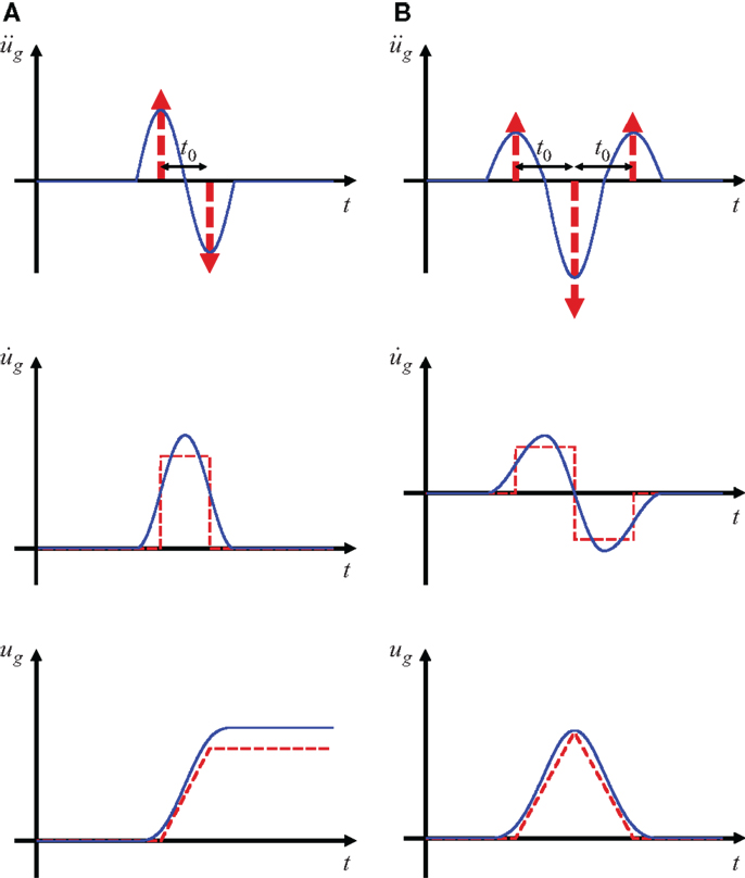
Figure 1. (A) Fling-step input and double impulse, (B) Forward-directivity input and triple impulse (Kojima and Takewaki, 2015b).
Consider a ground motion acceleration as triple impulse, as shown in Figure 1B, expressed by
where 0.5V is the given initial velocity and t0 is the time interval among three impulses. The comparison with the corresponding three wavelets of sinusoidal waves as a representative of the forward-directivity input of the near-fault ground motion (Mavroeidis and Papageorgiou, 2003; Kalkan and Kunnath, 2006) is also plotted in Figure 1B. The corresponding velocity and displacement of such triple impulse and three wavelets of sinusoidal waves are plotted in Figure 1B. The Fourier transform of of the triple impulse input can be derived as
SDOF System
Consider an undamped elastic-perfectly plastic SDOF system of mass m and stiffness k. The yield deformation and the yield force are denoted by dy and fy. Let , u and f denote the undamped natural circular frequency, the displacement (deformation) of the mass relative to the ground and the restoring force of the model, respectively. The time derivative is denoted by an over-dot.
Maximum Elastic–Plastic Deformation of SDOF System Subjected to Triple Impulse
The elastic–plastic response to the triple impulse can be described by the continuation of free-vibrations. The maximum deformation after the first impulse is denoted by umax1, that after the second impulse is expressed by umax2 and that after the third impulse is described by umax3 as shown in Figure 2. The input of each impulse is expressed by the instantaneous change of velocity of the structural mass. Such response can be derived by the combination of a simple energy approach and the solution of differential equations (equations of motion). The kinetic energy given at the initial stage (the time of the first impulse), that at the time of the second impulse, and the kinetic energy plus the elastic strain energy at the time of the third impulse are transformed into the sum of the hysteretic energy and the elastic strain energy corresponding to the yield deformation. Using this rule and incorporating the information from the equations of motion, the maximum deformation can be obtained in a simple manner. It should be noted that, while a simple and clear concept of critical input was defined in the case of double impulse (Kojima and Takewaki, 2015b), the criticality can be used only before the third impulse in the present triple impulse. This is because the timing of the third impulse, determined already for the first and second impulses, decreases the maximum deformation umax2 after the second impulse and may increase the maximum deformation umax3 after the third impulse. However, it is shown that this treatment of setting of timing provides the true criticality in an input level of practical interest.
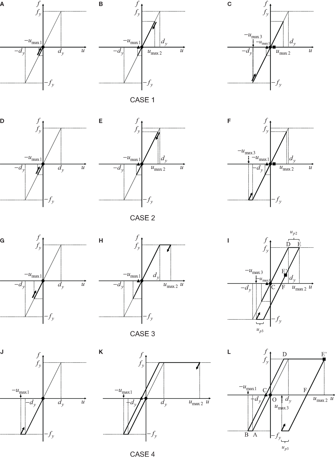
Figure 2. Prediction of maximum elastic–plastic deformation under triple impulse based on energy approach: (A–C) Case 1: elastic response, (D–F) Case 2: plastic response after the third impulse, (G–I) Case 3: plastic response after the second impulse, (J–L) Case 4: plastic response after the first impulse (•: first impulse, ▴: second impulse, ■: third impulse).
It should also be emphasized that, while the resonant equivalent frequency has to be computed for a specified input level by changing the excitation frequency in a parametric or mathematical programing manner in dealing with the sinusoidal input (Caughey, 1960; Liu, 2000; Moustafa et al., 2010), no iteration is required in the proposed method for the triple impulse. This is because the resonant equivalent frequency (resonance can be proved by using energy investigation: see Proof of Critical Timing in Appendix) can be obtained directly without the repetitive procedure (the timing of the second impulse can be characterized as the time with zero restoring force). It should be noted again that the resonance is defined before the third impulse.
Only critical response (upper bound) is captured by the proposed method and the critical resonant frequency can be obtained automatically for the increasing input level of the triple impulse. One of the original points in this paper is the introduction of the concept of “critical excitation” in the elastic–plastic response (Drenick, 1970; Abbas and Manohar, 2002; Takewaki, 2004, 2007; Moustafa et al., 2010; Kojima and Takewaki, 2015b). Once the frequency and amplitude of the critical triple impulse are computed, the corresponding three wavelets of sinusoidal waves as a representative of the forward-directivity motion can be identified.
Let us explain the evaluation method of umax1, umax2, and umax3. The plastic deformation after the first impulse is expressed by up1, that after the second impulse is described by up2, and that after the third impulse is denoted by up3. There are four cases to be considered depending on the yielding stage.
Case 1: elastic response during all response stages (umax3 is the largest).
Case 2: yielding after the third impulse (umax3 is the largest).
Case 3: yielding after the second impulse (umax2 or umax3 is the largest).
1: the timing of the third impulse is in the unloading stage.
2: the timing of the third impulse is in the yielding (loading) stage.
Case 4: yielding after the first impulse (umax2 is the largest).
In comparison with the double impulse, the triple impulse is quite difficult to derive the critical timing in a general case. This is because the timing of three impulses is fixed and there exist many complicated situations. In this paper, a case is treated where the critical timing is defined only before the third impulse. This means that, if the third impulse does not exist, timing gives the maximum value of umax2.
Case 1
Figures 2A–C show the maximum deformation after the first impulse, that after the second impulse, and that after the third impulse, respectively, for the elastic case (Case 1) during the whole stage. umax1 can be obtained from the energy conservation law.
On the other hand, since it can be proved that the critical timing of the second impulse to produce the maximum deformation umax2 is the time of zero restoring force (the proof similar to the Section “Proof of Critical Timing” in Appendix), umax2 can be computed from another energy conservation law.
In the elastic case, the critical timing of the second impulse is the time of zero restoring force and the velocity – V by the second impulse is added to the velocity −0.5V induced by the first impulse (full recovery at the zero restoring force due to zero damping).
Furthermore, since the timing of the third impulse is the time of zero restoring force, umax3 can be computed from another energy conservation law.
As explained above, the critical timing of the third impulse is the time of zero restoring force and the velocity 0.5V by the third impulse is added to the velocity 1.5V induced by the first and second impulses (full recovery at the zero restoring force due to zero damping).
It should be noted again that the critical timing t0 corresponds to the time of zero restoring force in Case 1 (see Proof of Critical Timing in Appendix). As a result, umax3 becomes the largest deformation among umax1, umax2, and umax3.
Case 2
Consider next the case (Case 2) where the model goes into the yielding stage after the third impulse. Figures 2D–F show the schematic response in this case. As in Case 1, umax1 can be obtained from the energy conservation law.
On the other hand, umax2 can be computed from another energy conservation law.
As stated above, the velocity – V by the second impulse is added to the velocity − 0.5V induced by the first impulse. Furthermore, umax3 can be computed from another energy conservation law.
As explained above, the velocity 0.5V by the third impulse is added to the velocity 1.5V induced by the first and second impulses. It should be noted that the critical timing t0 corresponds to the time of zero restoring force also in Case 2.
Case 3
Consider next the case (Case 3) where the model goes into the yielding stage after the second impulse. Figures 2G–I show the schematic response in this case. umax1 can be obtained from the energy conservation law.
As in Case 2, the critical timing of the second impulse is the time of zero restoring force. Although a more complicated discussion is needed to show this critical timing depending on the timing of the third impulse, it is omitted here. Case 3-1 and Case 3-2 (Figure 3) should be considered in Case 3. In Case 3-1, the timing of the third impulse is in the second unloading stage (Figures 2I and 3A).

Figure 3. Two different cases in Case 3: (A) Case 3-1, (B) Case 3-2 (•: first impulse, ▴: second impulse, ■: third impulse).
Case 3-1
In this case (Case 3-1), umax2 can be computed from another energy conservation law.
Then, umax2 can be expressed as
On the other hand, umax3 can be computed from another energy conservation law.
where νE′(<0) is the velocity at the time of third impulse (point E′) and ΔuE′F = uE′–up2 (uE′ (> 0): deformation at E′). up2 is characterized by up2 = umax2–dy and up3 satisfies umax2 + umax3 = 2dy + up3. νE′ and uE′ are characterized by Eqs 12 and 13 by solving the equation of motion.
In these equations, tEE′ = (T1/2)–(tCD + tDE) is the time interval between the first yielding termination point (E) and the third impulse (point E′), tCD = {Sin–1(2ω1dy/3V)}/ω1 is the time interval between the time of the second impulse and the time of the first yielding initiation (after the second impulse), and is the time interval between the time of the first yielding initiation (after the second impulse) and the time of the second unloading initiation. tCD and tDE are computed by solving the equations of motion and substituting the transition conditions (yielding and unloading conditions). In other words, umax3 can be obtained from
Then, umax3 can be expressed as
If the maximum deformation after the third impulse (corresponding to umax3) is positive, up3 is characterized by umax2 − umax3 = 2dy + up3. In this case, umax3 can be computed from another energy conservation law.
Then, umax3 can be expressed by
Case 3-2
In Case 3-2, the timing of the third impulse is in the yielding stage (Figure 3B). In this case (Case 3-2), umax2 is the deformation at the time of the third impulse (uE′) uE′ can be computed by solving the equation of motion and can be expressed by Eq. 15.
In this case, umax2 is given by
On the other hand, umax3 can be computed from another energy conservation law.
where νE′ is the velocity at the third impulse and up3 is characterized by umax2 − umax3 = 2dy + up3. νE′ is characterized by Eq. 18 by solving the equation of motion.
In these equations, tDE′= (T1/2)–tCD is the time interval between the first yielding initiation and the third impulse and tCD = {Sin–1(2ω1dy/(3V))}/ω1 is the time interval between the time of the second impulse (zero restoring force) and the time of the first yielding initiation (after the second impulse). tCD is computed by solving the equation of motion and substituting the transition conditions (yielding and unloading conditions). In other words, umax3 can be obtained from
Then, umax3 can be expressed by
Case 4
Consider finally the case (Case 4) where the model goes into the yielding stage even after the first impulse. Figures 2J–L show the schematic response in this case. umax1 can be obtained from the energy conservation law.
In this case (Case 4), umax2 is the deformation at the third impulse (uE′). uE′ can be computed by solving the equation of motion and uE′ can be obtained from Eq. 21.
In this case, umax2 is given by
On the other hand, umax3 can be computed from another energy conservation law.
where νE′ is the velocity at the third impulse and up3 is characterized by umax2 − umax3 = 2dy + up3. νE′ is characterized by Eq. 24 by solving the equation of motion.
In these equations, tDE′ = t0–tCD = (tOA + tAB + tBC)–tCD is the time interval between the second yielding initiation and the third impulse and t0 is the time interval between the time of the first impulse and the time of the second impulse. tOA = {Sin–1(2ω1dy/V)}/ω1 is the time interval between the time of the first impulse and the time of the first yielding initiation, is the time interval between the time of the first yielding initiation and the time of the first unloading initiation, tBC = T1/4 is the time interval between the time of the first unloading initiation and the time of the second impulse and tCD = {Sin–1(ω1dy/(ω1dy + V))}/ω1 is the time interval between the time of the second impulse and the time of the second yielding initiation. tOA, tAB, and tCD, are computed by solving the equation of motion and substituting the transition conditions (yielding and unloading conditions). In other words, umax3 can be obtained from
Then, umax3 can be expressed by
Figure 4 shows the plot of umax/dy = max (umax1/dy, umax2/dy, umax3/dy) with respect to the input level. 2Vy is the input level at which the maximum deformation after the first impulse just attain the yield deformation dy. Here, Vy is expressed by Vy = ω1dy. As stated before, there are four cases (Case 1–4).
Case 1: elastic response during all response stages (umax3 is the largest).
Case 2: yielding after the third impulse (umax3 is the largest).
Case 3: yielding after the second impulse (umax2 or umax3 is the largest).
Case 4: yielding after the first impulse (umax2 is the largest).
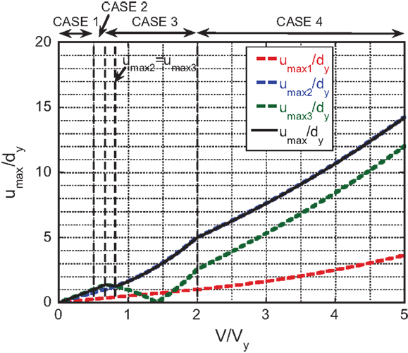
Figure 4. Maximum normalized elastic–plastic deformation under triple impulse with respect to input level.
In Case 1 and 2, umax3 is the largest. On the other hand, in Case 3, umax2 or umax3 is the largest and in Case 4, umax2 is the largest.
As observed in Figure 3, the timing of the third impulse sometimes decreases umax2. It may be useful to assume the timing of the third impulse at the zero restoring force in the unloading process as shown in Figure 5. In Case 1 and 2, this assumption is valid (see Figures 2C,F). Figure 6 presents the corresponding figure in which the timing of the third impulse is the time of zero restoring force after the attainment of umax2 (in the process of the second unloading). In Figure 6, four cases (Case 1*, Case 2*, Case 3*, Case 4*) are introduced corresponding to the previously defined four cases. Case 1* and Case 2* are Case 1 and Case 2 themselves. It can be understood, because the timing of the third impulse defined as the same interval between the first and second impulses decreases umax2, umax/dy in Case 4 in Figure 4 becomes smaller than that in Figure 6. However, it is noteworthy that umax/dy in Figure 6 can be a good upper bound of that in Figure 4 and umax/dy (umax2/dy) to any other timing t0 (except zero restoring force) does not become larger than that in Figure 6 (see Proof of Critical Timing and Upper Bound of Response Ductility via Relaxation of Timing of Third Impulse in Appendix).
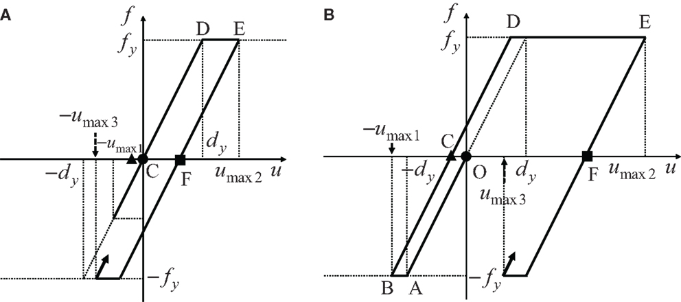
Figure 5. Modified version of timing of the third impulse: (A) Case 3, (B) Case 4 (•: first impulse, ▴: second impulse, ■: third impulse).
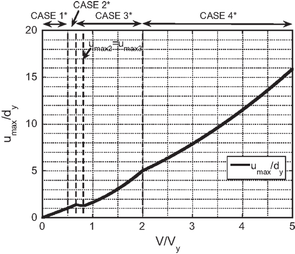
Figure 6. Maximum normalized elastic–plastic deformation under triple impulse with respect to input level (timing of the third impulse: zero restoring force).
Figure 7 presents the normalized timing t0/T1 (T1 = 2π/ω1) of the second impulse with respect to the input level. As stated before, this timing coincides with the time of zero restoring force after the first unloading (see Figure 2). It can be observed that the timing is delayed as the input level increases. It seems noteworthy to state again that only critical response giving the maximum value of umax2/dy (in case of the timing of the third impulse after the second unloading) is sought by the proposed method and the critical resonant frequency is obtained automatically for the increasing input level of the triple impulse. One of the original points in this paper is the tracking of the critical elastic–plastic response.
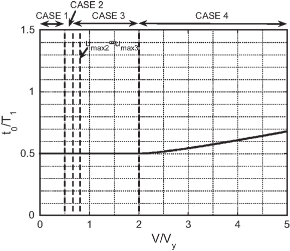
Figure 7. Interval time between the first and second impulses (the second and third impulses) with respect to input level.
Accuracy Check by Time–History Response Analysis Subjected to the Corresponding Three Wavelets of Sinusoidal Waves
In order to investigate the accuracy of using the triple impulse as a substitute of the corresponding three wavelets of sinusoidal waves (representative of the forward-directivity input), the time–history response analysis of the elastic–plastic SDOF model under the three wavelets of sinusoidal waves has been conducted.
In the evaluation procedure, it is important to adjust the input level of the triple impulse and the corresponding three wavelets of sinusoidal waves based on the equivalence of the Fourier amplitude. Figure 8 shows one example for the input level V/Vy = 3. Figures 9A,B illustrate the comparison of the ground displacement and velocity between the triple impulse and the corresponding three wavelets of sinusoidal waves for the input level V/Vy = 3. Only in Figures 8 and 9A,B, ω1 = 2π (rad/s)(T1 = 1.0 s) and dy = 0.16(m) are used.
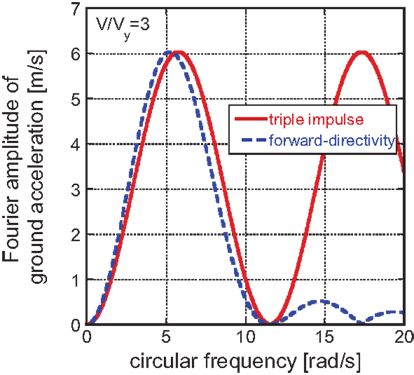
Figure 8. Adjustment of input level of triple impulse and the corresponding three wavelets of sinusoidal waves based on Fourier amplitude equivalence.
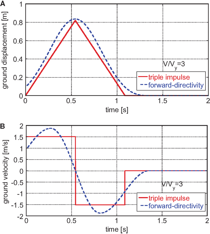
Figure 9. Comparison of ground displacement and velocity between triple impulse and the corresponding three wavelets of sinusoidal waves: (A) displacement, (B) velocity.
Figure 10 presents the comparison of the ductility (maximum normalized deformation) of the elastic–plastic structure under the triple impulse and the corresponding three wavelets of sinusoidal waves with respect to the input level. It can be seen that the triple impulse provides a good substitute of the three wavelets of sinusoidal waves in the evaluation of the maximum deformation if the maximum Fourier amplitude is adjusted appropriately.
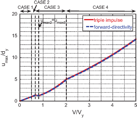
Figure 10. Comparison of ductility of elastic–plastic structure under triple impulse and the corresponding three wavelets of sinusoidal waves.
Figure 11 shows the comparison of the earthquake input energies by the triple impulse and the corresponding three wavelets of sinusoidal waves. An extremely accurate correspondence can be observed. This supports the validity of the triple impulse as a substitute of the forward-directivity near-fault ground motion.
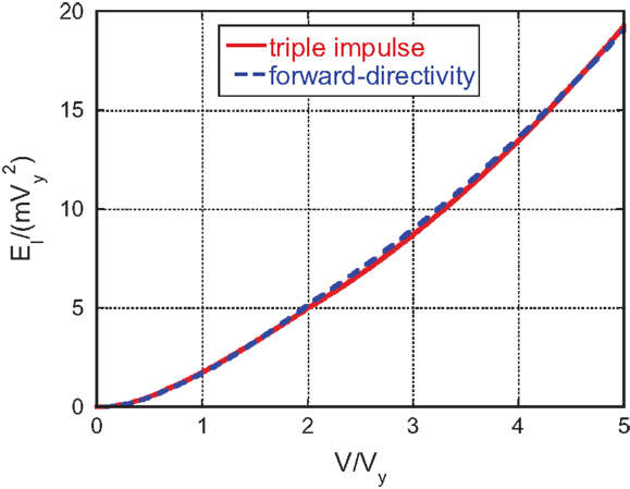
Figure 11. Comparison of earthquake input energies by triple impulse and the corresponding three wavelets of sinusoidal waves.
Figure 12 illustrates the comparison of response time histories (normalized deformation and restoring force) under triple impulse and those under the corresponding three wavelets of sinusoidal waves. The parameters ω1 = 2π (rad/s) (T1 = 1.0 s), dy = 0.16(m) are used here. While a rather good correspondence can be seen in general, the amplitude of deformation after the third impulse exhibits a slight difference resulting from the difference in timing of the third impulse. At the same time, a difference in phase can be observed both in the deformation and restoring force. This may also result from the difference in timing of the third impulse. The difference in the amount of energy input at the third impulse seems influence the later response.
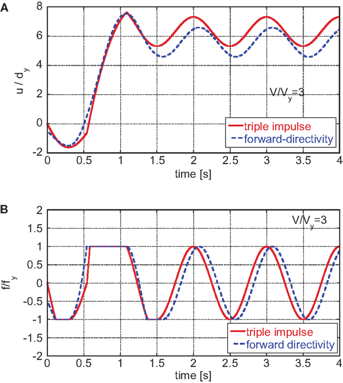
Figure 12. Comparison of response time history under triple impulse and that under the corresponding three wavelets of sinusoidal waves: (A) normalized deformation, (B) normalized restoring force.
Figure 13 presents the comparison of the restoring force characteristic under the triple impulse and that under the corresponding three wavelets of sinusoidal wave. The parameters ω1 = 2π (rad/s)(T1 = 1.0 s), dy = 0.16(m) are also used here. As seen in Figure 12, while the maximum deformations after the first and second impulses exhibit a rather good correspondence, the deformation response after the third impulse exhibits an unnegligible difference. However, since the deformation response after the third impulse does not affect the maximum deformation in an overall time range, this difference may not be significant.
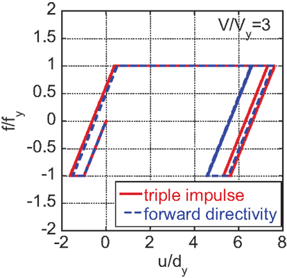
Figure 13. Comparison of restoring force characteristic under triple impulse and that under the corresponding three wavelets of sinusoidal waves.
Design of Stiffness and Strength for Specified Velocity and Period of Forward-Directivity Near-Fault Ground Motion Input and Response Ductility
As in the case of the double impulse as a substitute of the near-fault fling-step input, it may be meaningful to present a flowchart for design of stiffness and strength for the specified velocity and period of the near-fault forward-directivity input and response ductility. This design concept is based on the philosophy that, if we focus on the worst case of resonance, the safety for other non-resonant cases is guaranteed (Takewaki, 2002). This fact will be explained in the following section.
Since Figures 4 and 7 are non-dimensional ones, they can be used for such design. Figure 14 shows the flowchart for design of stiffness and strength. One example can be drawn as follows:
[Specified conditions] V = 2.00(m/s), t0 = 0.500(s), umax/dy = 4.00, m = 4.00 × 10⁶(kg)
[Design results] V/Vy = 1.70, Vy = 1.18(m/s), T1 = 1.00(s), dy = 0.188(m), k = 1.58 × 10⁸(N/m), fy = 2.97 × 10⁷(N)
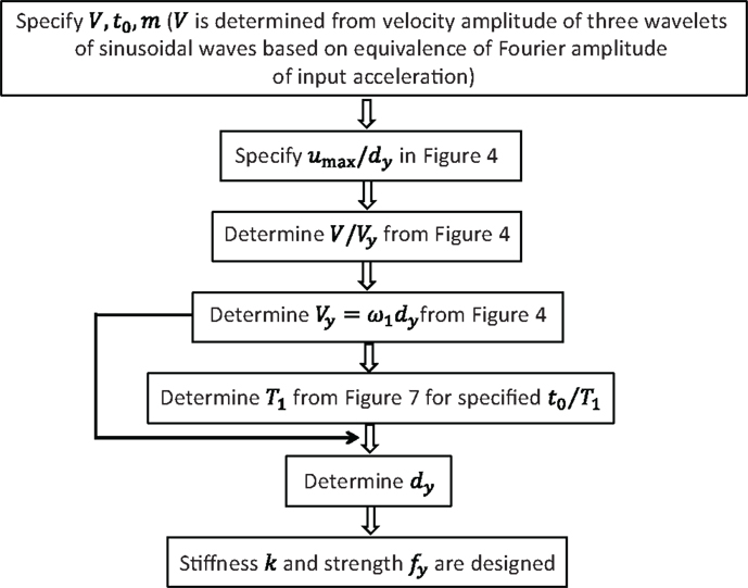
Figure 14. Flowchart for design of stiffness and strength.
From Figure 4, V/Vy = 1.70 can be obtained for the specified ductility umax/dy = 4.0. Then, Vy = 1.18(m/s) is derived from the specified condition V = 2.00(m/s) and V/Vy = 1.70. In the next step, T1 = 1.00(s) is found from Figure 7 for V/Vy = 1.70 and t0 = 0.5(s). In this model, dy = 0.188(m) is determined from Vy = ω1dy and T1 = (2π/ω1) = 1.00(s). Finally, k = 1.58 × 10⁸(N/m) is obtained from and fy = 2.97 × 10⁷(N) is derived by fy = kdy.
Approximate Prediction of Response Ductility for Specified Design of Stiffness and Strength and Specified Velocity and Period of Near-Fault Ground Motion Input
Until Section “Accuracy Check by Time–History Response Analysis Subjected to the Corresponding Three Wavelets of Sinusoidal Waves,” only the critical set of velocity and period of near-fault ground motion input and the corresponding critical response have been treated for a specified design of stiffness and strength. On the other hand, in Section “Design of Stiffness and Strength for Specified Velocity and Period of Forward-Directivity Near-Fault Ground Motion Input and Response Ductility,” the design flowchart of stiffness and strength for the specified velocity and period of the near-fault ground motion input and specified response ductility has been presented. In this section, an approximate prediction method of response ductility for specified design of stiffness and strength and specified velocity and period of near-fault ground motion input is explained. If a more exact response is desired then the response analysis for an arbitrary timing of impulses and an arbitrary input level can be done.
Figure 15 shows a schematic diagram of the approximate prediction method (only prediction of upper bound) of response ductility μ = umax/dy for a specified design of stiffness and strength and a specified velocity and period of near-fault ground motion input using the corresponding critical response. Generally, the specified set of velocity and period of near-fault ground motion input is not the critical set for a given structure. In such case, consider the critical set (point C) of velocity and period of input corresponding to the specified set of velocity. Let μA and μC denote the response ductilities corresponding to point A and C. From the Section “Proof of Critical Timing” in Appendix, μA < μC can be drawn directly. This enables an approximate prediction of response ductility (only upper bound) for a specified design of stiffness and strength and a specified velocity and period of near-fault ground motion input.
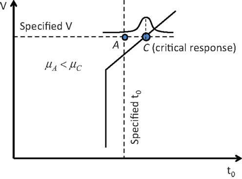
Figure 15. Schematic diagram of approximate prediction method of response ductility for specified design of stiffness and strength and specified velocity and period of near-fault ground motion input.
Conclusion
The conclusions may be summarized as follows:
(1) The triple impulse input has been introduced as a simplified version of the forward-directivity near-fault ground motion and a closed-form solution of the critical elastic–plastic response of a structure by this triple impulse input has been derived.
(2) It has been shown that, since only the free-vibration appears under such triple impulse input, the energy approach plays an important role in the derivation of the closed-form solution of a complicated elastic–plastic response. In other words, the energy approach enables the derivation of the maximum elastic–plastic seismic response. In this process, the input of impulse is expressed by the instantaneous change of velocity of the structural mass. The maximum elastic–plastic response after impulse can be obtained by equating the initial kinetic energy computed by the initial velocity to the sum of hysteretic and elastic strain energies. It has been shown that the maximum inelastic deformation can occur after either the second or third impulse depending on the input level.
(3) The validity and accuracy of the proposed theory have been investigated through the comparison with the response analysis result to the corresponding three wavelets of sinusoidal input as a representative of the forward-directivity near-fault ground motion. It has been made clear that, if the level of the triple impulse is adjusted so that its maximum Fourier amplitude coincides with that of the corresponding three wavelets of sinusoidal input, the maximum elastic–plastic deformation to the triple impulse exhibits a good correspondence with that to the three wavelets of sinusoidal wave.
(4) While the resonant equivalent frequency has to be computed for a specified input level by changing the excitation frequency in a parametric manner in dealing with the sinusoidal input, no iteration is required in the proposed method for the triple impulse. This is because the resonant equivalent frequency (resonance can be proved by using energy investigation) can be obtained directly without the repetitive procedure (the timing of the second impulse can be characterized as the time with zero restoring force). In the triple impulse, the analysis can be conducted without the input frequency (timing of impulses) before the second impulse. It should be noted that, while a simple and clear concept of critical input was defined in the case of double impulse (Kojima and Takewaki, 2015b), the criticality can be used only before the third impulse in the present triple impulse. This is because the timing of the third impulse, determined already for the first and second impulses, decreases the maximum deformation umax2 after the second impulse and may increase the maximum deformation umax3 after the third impulse.
(5) Only critical response (upper bound) is captured by the proposed method and the critical resonant frequency can be obtained automatically for the increasing input level of the triple impulse. Once the frequency and amplitude of the critical triple impulse are computed, the corresponding three wavelets of sinusoidal motion as a representative of the forward-directivity motion can be identified.
(6) A flowchart for design of stiffness and strength for the specified velocity and period of the near-fault ground motion input and response ductility has been proposed using the newly derived non-dimensional relations among response ductility, input velocity, and input period. It has been demonstrated that this flowchart can provide a useful result for such design.
(7) An approximate prediction method of response ductility (only prediction of upper bound) using the corresponding critical response can be developed for a specified design of stiffness and strength and a specified velocity and period of near-fault ground motion input.
Conflict of Interest Statement
The authors declare that the research was conducted in the absence of any commercial or financial relationships that could be construed as a potential conflict of interest.
Acknowledgments
Part of the present work is supported by the Grant-in-Aid for Scientific Research of Japan Society for the Promotion of Science (No. 24246095, No. 15H04079) and the 2013-MEXT-Supported Program for the Strategic Research Foundation at Private Universities in Japan (No. S1312006). This support is greatly appreciated.
References
Abbas, A. M., and Manohar, C. S. (2002). Investigations into critical earthquake load models within deterministic and probabilistic frameworks. Earthq. Eng. Struct. Dyn. 31, 813–832. doi: 10.1002/eqe.124.abs
Alavi, B., and Krawinkler, H. (2004). Behaviour of moment resisting frame structures subjected to near-fault ground motions. Earthq. Eng. Struct. Dyn. 33, 687–706. doi:10.1002/eqe.370
Bertero, V. V., Mahin, S. A., and Herrera, R. A. (1978). Aseismic design implications of near-fault San Fernando earthquake records. Earthq. Eng. Struct. Dyn. 6, 31–42. doi:10.1002/eqe.4290060105
Bray, J. D., and Rodriguez-Marek, A. (2004). Characterization of forward-directivity ground motions in the near-fault region. Soil Dyn. Earthq. Eng. 24, 815–828. doi:10.1016/j.soildyn.2004.05.001
Caughey, T. K. (1960). Sinusoidal excitation of a system with bilinear hysteresis. J. Appl. Mech. 27, 640–643. doi:10.1115/1.3644077
Hall, J. F., Heaton, T. H., Halling, M. W., and Wald, D. J. (1995). Near-source ground motion and its effects on flexible buildings. Earthq. Spectra 11, 569–605. doi:10.1193/1.1585828
Hayden, C. P., Bray, J. D., and Abrahamson, N. A. (2014). Selection of near-fault pulse motions. J. Geotech. Geoenviron. Eng. 140:04014030. doi:10.1061/(ASCE)GT.1943-5606.0001129
Kalkan, E., and Kunnath, S. K. (2006). Effects of fling step and forward directivity on seismic response of buildings. Earthq. Spectra 22, 367–390. doi:10.1193/1.2192560
Kalkan, E., and Kunnath, S. K. (2007). Effective cyclic energy as a measure of seismic demand. J. Earthq. Eng. 11, 725–751. doi:10.1080/13632460601033827
Khaloo, A. R., Khosravi1, H., and Hamidi Jamnani, H. (2015). Nonlinear interstory drift contours for idealized forward directivity pulses using “Modified Fish-Bone” models. Adv. Struct. Eng. 18, 603–627. doi:10.1260/1369-4332.18.5.603
Kojima, K., Fujita, K., and Takewaki, I. (2015a). Critical double impulse input and bound of earthquake input energy to building structure. Front. Built Environ. 1:5. doi:10.3389/fbuil.2015.00005
Kojima, K., and Takewaki, I. (2015b). Critical earthquake response of elastic-plastic structures under near-fault ground motions (Part 1: Fling-step input). Front. Built Environ. 1:12. doi:10.3389/fbuil.2015.00012
Liu, C.-S. (2000). The steady loops of SDOF perfectly elastoplastic structures under sinusoidal loadings. J. Mar. Sci. Technol. 8, 50–60.
Mavroeidis, G. P., Dong, G., and Papageorgiou, A. S. (2004). Near-fault ground motions, and the response of elastic and inelastic single-degree-freedom (SDOF) systems. Earthq. Eng. Struct. Dyn. 33, 1023–1049. doi:10.1002/eqe.391
Mavroeidis, G. P., and Papageorgiou, A. S. (2003). A mathematical representation of near-fault ground motions. Bull. Seismol. Soc. Am. 93, 1099–1131. doi:10.1785/0120020100
Moustafa, A., Ueno, K., and Takewaki, I. (2010). Critical earthquake loads for SDOF inelastic structures considering evolution of seismic waves. Earthq. Struct. 1, 147–162. doi:10.12989/eas.2010.1.2.147
Mukhopadhyay, S., and Gupta, V. K. (2013a). Directivity pulses in near-fault ground motions – I: identification, extraction and modeling. Soil Dyn. Earthq. Eng. 50, 1–15. doi:10.1016/j.soildyn.2013.02.017
Mukhopadhyay, S., and Gupta, V. K. (2013b). Directivity pulses in near-fault ground motions – II: estimation of pulse parameters. Soil Dyn. Earthq. Eng. 50, 38–52. doi:10.1016/j.soildyn.2013.02.019
Rupakhety, R., and Sigbjörnsson, R. (2011). Can simple pulses adequately represent near-fault ground motions? J. Earthq. Eng. 15, 1260–1272. doi:10.1080/13632469.2011.565863
Sasani, M., and Bertero, V. V. (2000). “Importance of severe pulse-type ground motions in performance-based engineering: historical and critical review,” in Proceedings of the Twelfth World Conference on Earthquake Engineering (Auckland).
Takewaki, I. (2002). Robust building stiffness design for variable critical excitations. J. Struct. Eng. ASCE 128, 1565–1574. doi:10.1061/(ASCE)0733-9445(2002)128:12(1565)
Takewaki, I. (2004). Bound of earthquake input energy. J. Struct. Eng. ASCE 130, 1289–1297. doi:10.1061/(ASCE)0733-9445(2004)130:9(1289)
Takewaki, I. (2007). Critical Excitation Methods in Earthquake Engineering, 2nd Edn. Oxford: Elsevier, 2013.
Takewaki, I., Moustafa, A., and Fujita, K. (2012). Improving the Earthquake Resilience of Buildings: The Worst Case Approach. London: Springer.
Takewaki, I., and Tsujimoto, H. (2011). Scaling of design earthquake ground motions for tall buildings based on drift and input energy demands. Earthq. Struct. 2, 171–187. doi:10.12989/eas.2011.2.2.171
Vafaei, D., and Eskandari, R. (2015). Seismic response of mega buckling-restrained braces subjected to fling-step and forward-directivity near-fault ground motions. Struct. Des. Tall Spec. Build. 24, 672–686. doi:10.1002/tal.1205
Xu, Z., Agrawal, A. K., He, W.-L., and Tan, P. (2007). Performance of passive energy dissipation systems during near-field ground motion type pulses. Eng. Struct. 29, 224–236. doi:10.1016/j.engstruct.2006.04.020
Yamamoto, K., Fujita, K., and Takewaki, I. (2011). Instantaneous earthquake input energy and sensitivity in base-isolated building. Struct. Des. Tall Spec. Build. 20, 631–648. doi:10.1002/tal.539
Yang, D., and Zhou, J. (2014). A stochastic model and synthesis for near-fault impulsive ground motions. Earthq. Eng. Struct. Dyn. 44, 243–264. doi:10.1002/eqe.2468
Zhai, C., Chang, Z., Li, S., Chen, Z.-Q., and Xie, L. (2013). Quantitative identification of near-fault pulse-like ground motions based on energy. Bull. Seismol. Soc. Am. 103, 2591–2603. doi:10.1785/0120120320
Appendix
Proof of Critical Timing
In comparison with the double impulse, the triple impulse is quite difficult to derive the critical timing in a general case. This is because the timing of three impulses is fixed and there exist many complicated situations. In this paper, a case is treated where the critical timing is defined only before the third impulse. This means that, if the third impulse does not exist, timing gives the maximum value of umax2. The following explanation is the same as in the previous paper for the double impulse.
Consider the critical timing of the second impulse. Let νc denote the velocity of the mass passing the zero restoring force (zero elastic strain energy) after the first unloading and ν*, u* denote the velocity and the elastic deformation component at an arbitrary point between the first unloading and the second yielding. Since the first unloading starts from the state with zero velocity and the elastic strain energy fydy/2, the relation holds. From the energy conservation law between the first unloading and the second yielding, the relation mν*2/2 + ku*2/2 = fydy/2 holds. Consider the second impulse at the same time of the state of ν*,u*. The total mechanical energy can be expressed by m(ν* + V)2/2 + ku*2/2. Since the relation m(ν* + V)2/2 + ku*2/2 = mν*2/2 + ku*2/2 + mν*V +mV2/2 = fydy/2 + mν*V + mV2/2 holds and the maximum deformation after the second yielding is caused by the maximum total mechanical energy, the maximum velocity ν* causes the maximum deformation after the second yielding. This timing is the zero restoring force after the first unloading. This completes the proof.
Upper Bound of Response Ductility via Relaxation of Timing of Third Impulse
The case is treated here where the third impulse acts at the timing of zero restoring force in the second unloading process. It can be shown that this case provides the larger maximum deformation umax2 than the case treated before (the same timing between the first and second impulses).
Consider the case where the model goes into the yielding stage even after the first impulse. The case where the model goes into the yielding stage after the second impulse (elastic after the first impulse) can be explained in almost the same manner. Figure 5B shows the schematic response in this case. umax1 can be obtained from the energy conservation law.
On the other hand, umax2 can be computed from another energy conservation law.
where νc is characterized by and up2 is characterized by umax2 + (umax1–dy) = dy + up2. In other words, umax2 can be obtained from
Furthermore, umax3 can be computed from another energy conservation law.
where up3 is characterized by −umax3 + (umax2 – dy) = dy + up3. In other words, umax3 can be obtained from
Keywords: earthquake response, critical response, elastic–plastic response, ductility factor, near-fault ground motion, forward-directivity input, triple impulse
Citation: Kojima K and Takewaki I (2015) Critical earthquake response of elastic–plastic structures under near-fault ground motions (Part 2: Forward-directivity input). Front. Built Environ. 1:13. doi: 10.3389/fbuil.2015.00013
Received: 23 June 2015; Accepted: 16 July 2015;
Published: 03 August 2015
Edited by:
Nikos D. Lagaros, National Technical University of Athens, GreeceReviewed by:
Johnny Ho, The University of Queensland, AustraliaSameh Samir F. Mehanny, Cairo University, Egypt
Copyright: © 2015 Kojima and Takewaki. This is an open-access article distributed under the terms of the Creative Commons Attribution License (CC BY). The use, distribution or reproduction in other forums is permitted, provided the original author(s) or licensor are credited and that the original publication in this journal is cited, in accordance with accepted academic practice. No use, distribution or reproduction is permitted which does not comply with these terms.
*Correspondence: Izuru Takewaki, Department of Architecture and Architectural Engineering, Graduate School of Engineering, Kyoto University, Kyotodaigaku-Katsura, Nishikyo, Kyoto 615-8540, Japan, takewaki@archi.kyoto-u.ac.jp