Automatic Filtering of Soil CO₂ Flux Data; Different Statistical Approaches Applied to Long Time Series

Introduction

Volcanic gas emissions may occur as visible manifestations, such as fumaroles, gas vents, and bubbling springs, or as invisible emissions through diffuse degassing (Fischer and Chiodini, 2015 and references therein). The degassing phenomena characterize the volcanic systems both during eruptive and quiescent periods of activity. Studies of these permanent and silent gas emissions started to be performed in the early nineties in Italian volcanoes (Baubron et al., 1990; Allard et al., 1991). The permanent soil CO₂ flux networks that have been set up in various volcanic areas of the world since then (Mori et al., 2002; Salazar et al., 2002; Granieri et al., 2003, 2010; Gurrieri et al., 2008; Padrón et al., 2008; Viveiros et al., 2008, 2015a; Hernández et al., 2012; Liuzzo et al., 2013; Laiolo et al., 2016) already contributed to identify geochemical signs that represent changes on the volcanic activity, namely by recognizing volcanic unrest episodes (Granieri et al., 2003, 2010; Salazar et al., 2004; Pérez et al., 2006) or as precursors of eruptive periods (Brusca et al., 2004; Carapezza et al., 2004; Aiuppa et al., 2010; Pérez et al., 2012; Liuzzo et al., 2013; Inguaggiato et al., 2017). Some gas flux anomalies were also associated with seismic activity (Salazar et al., 2002) and the stations installed have also been used as proxy for indoor environments and showed to be useful for risk assessment in diffuse degassing areas (Viveiros et al., 2009, 2015b).

Despite all the useful information obtained with these stations for the seismo-volcanic monitoring, the recorded soil CO₂ flux values have showed that gas fluxes are highly influenced by environmental factors, such as meteorological changes, which can be responsible for more than 50% of the gas flux variations (Granieri et al., 2003, 2010; Viveiros et al., 2009, 2015a). Different statistical methodologies have been applied to filter the recorded CO₂ time series in order to remove the external influences and produce a gas flux sign that may represent deep changes (e.g., Granieri et al., 2003; Viveiros et al., 2008, 2015a; Cannata et al., 2010; Liuzzo et al., 2013; Lelli and Raco, 2017). Several studies have also highlighted the existence of cyclic variations on the CO₂ flux time series with both daily and seasonal oscillations (Granieri et al., 2003; Padrón et al., 2008; Hernández et al., 2012; Rinaldi et al., 2012; Viveiros et al., 2014), even if only few of them attempt to model and explain the variations observed (Rinaldi et al., 2012; Viveiros et al., 2014). Even if most of the studies highlight the impact that meteorological changes may have on the soil gas fluxes, the use of raw data as routine in the volcano observatories is still common and may result in biased interpretations. The current study uses data from a permanent soil CO₂ flux station installed in 2010 in a geothermal area in the north flank of the active Fogo central volcano (São Miguel Island). This study will apply for the first time different statistical approaches to the data recorded by GFOG4 station, and will constitute an opportunity to discuss the results, highlight positive aspects and limitations, and to select an adequate methodology to filter the raw data. Despite the fact that several filtering techniques have been already applied to soil CO₂ flux time series, the present study focuses on an automatic filtering that may be used as routine in the volcano observatories to identify anomalous gas values and contribute to recognize unrest episodes.

Characterization of the Study Area

Fogo is a polygenetic volcano located in the central part of São Miguel Island (Azores archipelago, Portugal) and has a summit caldera with maximum diameter of about 3.2 km (Wallenstein et al., 2015 and references therein). The volcanic edifice started to form more than 200 ka ago (Muecke et al., 1974) and the last intracaldera magmatic eruption occurred after the settlement of the island, in 1563, and was of sub-Plinian type. This explosive event was followed four days later by a basaltic eruption in the north flank of the volcano (Wallenstein et al., 2015). The main tectonic structures that cross this volcanic system show a dominant NW-SE trend, the same as the Ribeira Grande graben that dominates the north flank of the volcano (Carmo et al., 2015). Since 2003 several seismic swarms have affected the central area of São Miguel, namely Fogo and Congro volcanic systems (Silva et al., 2012). During the period under analysis in the current study a total of 4,479 seismic events were recorded by the CIVISA seismic network for the Fogo Volcano seismogenic area (Silva, 2011 and references therein). Maximum local magnitude (M_L) was 2.9 from an earthquake recorded on 29th April 2012 (CIVISA catalog: http://www.ivar.azores.gov.pt/civisa/Paginas/homeCIVISA.aspx).

Nowadays the volcanic activity in the area is characterized not only by seismic swarms (Silva et al., 2012), but also by episodes of ground deformation (Okada et al., 2015) and the presence of secondary manifestations of volcanism, such as three main hydrothermal fumarolic fields (Caldeira Velha, Caldeiras da Ribeira Grande and Pico Vermelho), thermal and cold CO₂-rich springs, as well as, several diffuse degassing areas (Ferreira et al., 2005; Caliro et al., 2015; Viveiros et al., 2015b). These manifestations are essentially found out in the north flank of the volcano, and seem to be tectonically controlled by the graben faults. Submarine gas emissions are also found out in the volcano area and are dominated by high CO₂ emissions.

A permanent soil CO₂ flux network started to be implemented in this volcanic system in February 2002 with the installation of the so-called GFOG1 station in the Pico Vermelho geothermal power plant area (Viveiros et al., 2008). The network expanded in May 2005 when a second soil CO₂ flux station was installed inside the Fogo caldera in an area with low CO₂ emissions, and the main goal was to evaluate changes that could be correlated with the unrest episode that was affecting Fogo-Congro volcanic systems (Viveiros et al., 2015a). During 2010 a new degassing anomaly developed in the area surrounding Caldeiras da Ribeira Grande fumarolic field, caused by the drilling of a geothermal well. A multidisciplinary monitoring programme was set up in the area aiming not only to evaluate the expansion of the anomaly zone but also to identify possible signs that could represent deep processes and changes on the gas pressure that could end up in hazardous situations. A permanent soil CO₂ flux station, named GFOG4, was installed in the area in June 2010 as part of the monitoring programme.

Methodology

Sampling and Data Acquisition

GFOG4 is a permanent automatic station that measures soil CO₂ flux and is part of the IVAR/CIVISA seismic-volcanic monitoring network. The station performs measurements based on the “time 0, depth 0” accumulation chamber method (Chiodini et al., 1998). The soil CO₂ flux measurement is made once every hour by lowering the chamber into the ground and by pumping the gases into an infrared gas analyzer (Dräeger detector, maximum scale 30 vol.%). The soil CO₂ flux is computed as the linear best fit of the flux curve over a predefined period of time. This method allows the measurement of the flux independently from the transport regime and the soil properties (Chiodini et al., 1998).

The station also has meteorological and soil sensors, which simultaneously acquire data related to atmospheric pressure, air, and soil temperatures, relative air humidity, wind speed and direction, rainfall, and soil water content. Thermo hygrometers and wind sensors are set about 1 m above the ground, whereas soil water content and soil temperature sensors give measurements at a depth of about 30 cm (Viveiros et al., 2015b). For additional details about the methodology and the characteristics of the equipment see Viveiros et al. (2015b).

The 2 years of data acquisition, between January 2013 and December 2014, was the period selected to apply the statistical methodologies and to understand the CO₂ flux variations for this monitoring site. This selected period was taken from the middle of the whole recorded period (June 2010–June 2017). The periods between June 2010 and December 2012, as well as, between January 2015 and June 2017 were used to check the adequacy of the models proposed.

Statistical Data Treatment

Stepwise Multiple Linear Regression

Previous studies (Granieri et al., 2003, 2010; Viveiros et al., 2008) applied multiple linear regression analysis (Draper and Smith, 1981) to the data in order to build a model that can explain the CO₂ flux variations. This regression is normally used when there is the need to explain the relationship between one dependent variable and two or more independent variables. In this case, the dependent variable is the CO₂ flux and the independent variables are chosen from the environmental factors measured by the station. The model follows Equation(1),

Where β₀ is the intercept, β_n are the coefficients or the slope of the independent variables, x_n the measured environmental factors and y is the predicted CO₂ flux.

When building the model Neter et al. (1983) advice to choose independent variables in order that the regression model is as complete and realistic as possible, so the adequate prediction is reached. However, a balance is needed and the regression model must include only the relevant variables because the irrelevant ones decrease the precision of the predicted values, and increase the complexity of the model.

To determine, within a multiple regression model, if a particular factor (x_i) is making a contribution to the model, it is tested the hypothesis that the value of that coefficient is zero: H₀: β_i = 0; H_A: β_i≠ 0.

The null hypothesis says that a change in the value of x_i would neither linear increase or decrease y, meaning, y and x_i are not linearly related. To test these hypotheses the p-values for all coefficients in the model are determined and are based on a t-statistic, where the t score (t*) is calculated (Neter et al., 1983) as:

If the p-value for a coefficient is higher than 0.05 the variable for that coefficient can be omitted, for a 95% confidence interval. The application of this parametric methodology requires that populations follow the normal distribution (Draper and Smith, 1981).

Because multiple linear regression involves multiple variables, omitting a variable can be challenging, Pardoe et al. (2018) warn us that this test only suggests that one variable is not needed in a model with all the other variables included. For example, if we have more than one variable with a p-value higher than 0.05, by omitting one of those variables, a new model without that variable must be considered because the other variables can now have significance.

An alternative method to identify a good subset of variables to include in the model, with considerably less computing than what is required for all possible regressions, is the Stepwise Multivariate Regression method. Rawlings et al. (1998) explain that these subset models are identified sequentially by adding or deleting the variable that has the greatest impact on the residual sum of squares. These stepwise methods are not guaranteed to find the “best” subset for each subset size, and the results produced by different methods may not agree with each other. This method consists of a forward stepwise selection, which chooses variables by adding one variable at a time to the previously chosen subset model. It starts by choosing the independent variable that accounts for the largest amount of variation in the dependent variable. At each successive step, it adds the variable that causes the largest decrease in the residual sum of squares. Forward selection continues until all variables are in the model. A backward elimination of variables, which starts with a full model and then eliminates, at each step, the variable whose deletion will cause the residual sum of squares to increase the least. Backward elimination continues until the subset model contains only one variable.

Neither forward selection nor backward elimination takes into account the effect that the addition or deletion of a variable can have on the contributions of the other variables to the model. A variable early added to the model can lose importance after other variables are added, or variables previously eliminated can become important after other variables are removed from the model. So, Stepwise Regression is a forward selection process that rechecks at each step the importance of all previously included variables and, if there is a variable that does not meet the minimum criterion, it changes the procedure to backward elimination and variables are dropped one at a time until all remaining variables meet the minimum criterion. Then, forward selection resumes. This process continues until the adding or the removing of variables does not meet the minimum criterion. Normally this criterion comes in form of a F-Test (Rawlings et al., 1998).

All the variables that increase more than 1% the explanatory power of the model are inserted in the model. Additional details about the methodological approach and criteria used to select the variables that fit in the model are found out in Viveiros et al. (2015a). Predicted and residuals values are calculated based on the proposed model. The Stepwise Multivariate Regression Analysis was applied using the MATLAB^® software, version 2017b.

Spectral Analysis

Discrete Fast Fourier Transform

Previous soil CO₂ flux studies used the Fourier Transform as the method to identify potential periodicities on the analyzed datasets (Padrón et al., 2008; Hernández et al., 2012; Rinaldi et al., 2012; Viveiros et al., 2014). The Fourier Transform is a method to transform a time domain function into frequency domain. It decomposes any periodic function in a sum of cosines and sines of different frequencies making it a good tool to identify harmonic oscillations. It is a complex-valued function, whose absolute value represents the intensity of a frequency present in the function.

Because the data in this work is a finite time series of samples, i.e., discrete values, the Discrete Fourier Transform (DFT) is used. It will transform a finite sequence of equally spaced samples of a time domain function into a sequence of complex numbers on frequency domain. With N samples of input, we will have N independent values of output. Each output value corresponds to the intensity of a frequency.

To chose the adequate sampling rate, Press et al. (1992) explain that there is a special frequency, the Nyquist critical frequency, given by f = 1/2Δ, where Δ is the sampling interval. This frequency corresponds to the value of N/2 and it means that every frequency higher than f will be somewhat falsely translated into the frequencies lower than f. To overcome this problem, the sample rate must be, at least, the double of the maximum frequency to be measured, so that two points per cycle of that frequency are present. Also, the output of a DFT will repeat itself after N/2.

By definition the DFT (H) is given by Equation (2) and its inverse by Equation (3):

where N is the number of samples, h_n a discrete time series and e^−i2πkn/N is the Euler's formula, which states that e^i2πkn/N = cos(2πkn/N) + i sin(2πkn/N).

Unfortunately DFT is a computational intensive algorithm and a powerful computer is not always available. So, a more efficient algorithm, the Fast Fourier Transform (FFT), will be used to simplify the calculation of the Discrete Fourier Transform and its inverse. The calculation of the DFT by definition and for a data sequence with N points has an order of N² arithmetic operations, but with the help of a FFT algorithm, it computes the same result having an order of N.log(N) operations as shown in Cooley and Tukey (1965). The difference in calculation time may be substantial, especially for a large set of data.

There are many different algorithms that can be called FFT, but the most widely used is the Radix-2 Decimation in Time algorithm by Cooley and Tukey (1965). This algorithm divides a N size transform into two N/2 dimension intervals in each calculation step. It first calculates the transform of the even index elements and then the odd index elements, and then combines the two results to produce the Fourier transform of the sequence. This idea can be made recursively to reduce calculation time. This simplification assumes that N is a power of two (2ⁿ), but since it is usually possible to choose the number of points to use or to pad the end of the time series with zeros, this restriction is not a major problem.

To decompose the local time-frequency of a waveform, a Windowed Fourier Transform is used. Because the transform is performed on a segment of constant time through a time series at a constant step, the transform will have a constant time frequency resolution and discontinuities will exist between the function at the start and finish of the window. Those discontinuities will cause the transform to develop non-zero values at frequencies that do not exist. This is commonly called spectral leakage (Mallat, 2009). In order to reduce this problem the waveform is multiplied by a windowing function that decreases smoothly from one at its center to zero at its ends. Also to change the resolution, the window size needs to be changed. The choice of a particular window size depends on the desired resolution trade-off between time and frequency (Mallat, 2009). There are many different choices of windowing functions and the one used in the present study was the Hanning, which was already applied previously by Viveiros et al. (2014) to similar datasets.

Wavelet Transform

Some studies performed on SO₂ and CO₂ flux time series recorded from different volcanoes plumes used wavelet analyses to identify potential cyclic variations (Boichu et al., 2010; Pering et al., 2014). Similarly to the Fourier analysis, wavelet analysis is also a method to decompose a time series into time-frequency, but instead of using a sum of cosines and sines, it uses special made functions to have specific properties, such as better frequency localization or better transient localization that make them useful for signal processing (Mallat, 2009).

Mallat (2009) highlights that wavelets request less coefficients to represent local transient structures, which leads to a fast computational algorithm comparing to the FFT. In addition, wavelets are less affected by the lack of data, which allows an easier analysis of long time series. Another drawback of FFT analysis is that the time information may be lost in the transform since, depending on the window's size, it may be difficult to tell when an event took place. Wavelet analysis is thus becoming a common tool for analyzing localized variations within a time series (Torrence and Compo, 1998). Wavelet transform also has continuous and discrete transforms, but, to analyze how the frequency content of a signal changes over time the continuous transform is the most used. Farge (1992) states that the continuous wavelet transform is better suited because its redundancy allows good legibility of the signal's information content.

The formulation of the continuous wavelet transform (CWT) (Wx) was developed by Grossmann and Morlet (1984) and for a function x(t) is expressed by Equation (4):

where, s corresponds to the wavelet scale, u to the shift parameter and t is the time component.

Because this work uses discrete time series, Equation (5), defined by Torrence and Compo (1998), consists of the continuous wavelet transform of a discrete sequence x_n as the convolution of x_n with a scaled and translated version of a wavelet function ψ₀ (η):

where the (ψ*) indicates the complex conjugate of the wavelet. By varying the wavelet scale s and translating along the localized time index n for a time step δt, it is possible to construct a graphic similar to a spectrogram, called scalogram, showing the amplitude power vs. the scale and how this amplitude varies with time. These calculations can be very computational intensive but they are considerably fast to do if they are done in the Fourier space (for additional details, see Torrence and Compo, 1998).

One of the criticism about using wavelet analyses is related with the randomness associated with the selection of the wavelet function, ψ. Choosing the wavelet function depends on the final objectives of the data analysis. In this work, the goal is to perform a time-frequency analysis. MATLAB^® was used to perform the wavelet analysis and the wavelet function supported by MATLAB^® that was used, was the bump wavelet because it provides good frequency localization. The Fourier transform of the bump wavelet with parameters σ and μ, is defined in Meignen et al. (2012) and is expressed by Equation (6):

Where ξ is a real value and χ is the indicator function for the interval [μ−σ, μ+σ]. In this last case, χ is 1 if inside the interval and 0 if lays outside. By default, the values of the parameters used by MATLAB are μ = 5 and σ = 0.6. Another option could have been the Morlet wavelet, also available on the MATLAB's wavelet analysis toolbox, which exhibits poorer frequency localization than the bump wavelet, but superior time localization, making it a better choice for transient localization.

By using FFT, one can obtain the spectrum of the data; however, with wavelets, Shu and Qinyu (2005) demonstrated that the global wavelet spectrum on some occasions did not provide the correct results, especially when there are sharp peaks in the power spectrum. This happens because the global wavelet spectrum at small wavelets (high frequencies) will smooth the spectrum and at large wavelet scales (low frequencies) the peaks are sharper and have a higher amplitude. Shu and Qinyu (2005) state that because there is the need to know whether there are sharp peaks in the time series prior to this spectral analysis, the Fourier spectrum might be a better choice for this type of analysis.

Residuals Filtering

When cycles are identified in the time series, to remove unwanted cycles from the datasets (high frequencies) and reveal the constants components (low frequencies), a low pass filter may be used (Sedra and Smith, 2004). FFT was already applied in previous studies (Viveiros et al., 2014) and can be used for filtering since the signal may be converted between the time and the frequency domain. In order to apply a filter, one has to transform the signal into the frequency domain, apply the filter by zeroing the unwanted part of the spectrum, and transform it back into the time domain. But FFT filtering would imply high computational tasks and a high number of samples to be considered for filtering, increasing latency, and if the continuity of the waveform is no longer guaranteed artifacts will appear. For this reason, for time series with identified cyclic behavior, the application of other type of filtering, such as continuous-time filters, is suggested. Within this type of filters, one can choose from different families of filters, such as Chebyshev filter, which has the best approximation to the ideal response but with the cost of adding ripples, or the Butterworth filter that has a more flat frequency response. For this reason, this last type of filter is preferable to a Chebyshev filter (Jurišić et al., 2002).

Results

The data analyzed in this work were collected from June 2010 to June 2017 (Figure 1). During this period the CO₂ flux varied between 0.37 and 6,606 g m⁻²d⁻¹, with a mean of 1,165 gm⁻² d⁻¹ (Table 1). The permanent station is also installed in a thermal anomalous zone with soil temperature varying around 32.2°C and maximum recorded values for the whole period was 47.2°C (Table 1). Several spike-like variations are observed on the soil CO₂ flux time series and seasonal cycles with higher CO₂ emissions recorded during winter period are also observed. Higher scatter on the recorded data is also observed on the winter period when compared to the summer (Figure 1).

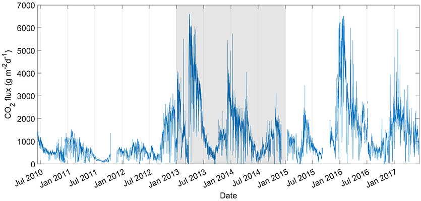
Figure 1. Soil CO₂ flux data acquired in GFOG4 during the period June 2010–June 2017. The gray area represents the period used to produce the explanatory regression model.

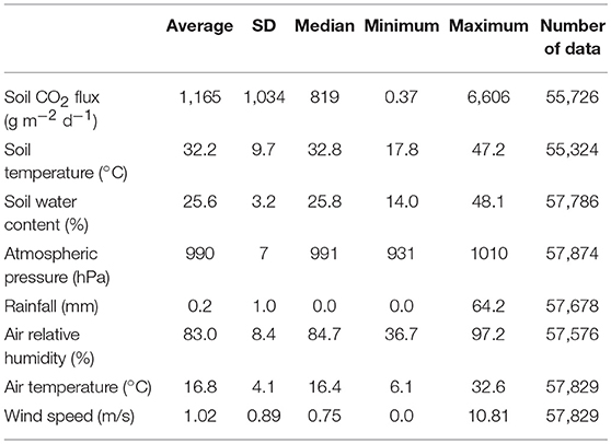
Table 1. Descriptive statistics of the data acquired in GFOG4.

Building a Model

As mentioned above, the period selected for the construction of the explanatory model corresponded to 2 years of data, from January 2013 to December 2014. Figure 2 shows the soil CO₂ flux and the various environmental time series recorded by the permanent station. Detailed analyses of the figure shows that some variables seem to correlate inversely with the soil CO₂ flux, namely the air (Figure 2a) and soil temperature (Figure 2c). On the other hand, soil water content (Figure 2b) shows in general similar variations as the soil CO₂ fluxes. Pearson correlation coefficients confirm these observations (Figure 3), with soil temperature showing the highest inverse correlation (−0.63) with the soil CO₂ flux. For the other side, soil water content is the variable with highest direct correlation (0.56) with the gas flux. Rainfall is the least influential variable with a correlation of just 0.05.

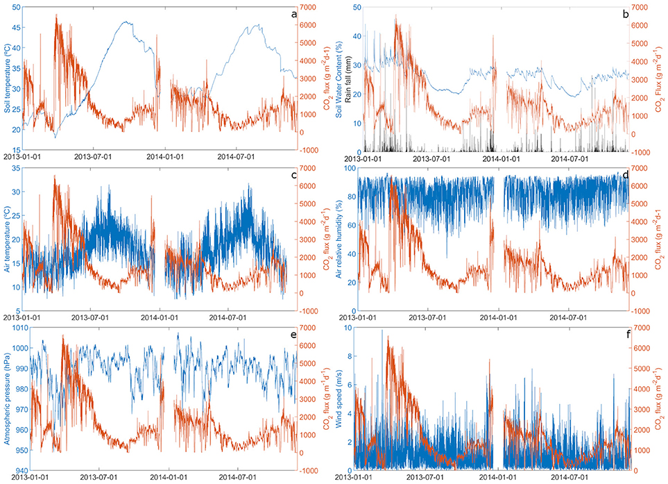
Figure 2. Environmental and soil CO₂ flux time series for the period selected to build the regression model (2013–2014). Orange lines represent the soil CO₂ flux in all graphics, black line the rainfall (b), and the blue lines the other monitored environmental variables, from (a–f) soil temperature, soil water content, air temperature, air relative humidity, atmospheric pressure and wind speed.

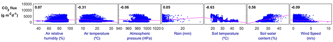
Figure 3. Pearson correlation coefficients between soil CO₂ flux and the monitored environmental variables. Blue points correspond to the environmental variables vs. the soil CO₂ flux and the pink lines are the correlation trendlines.

The stepwise regression model selected is the number 4 (Table 2), which accounts with the air and soil temperature, wind speed, and soil water content as the explanatory variables to be included in the model. Before applying the stepwise model, several partial regression models were tested, but theoretically the same result can be obtained in a much faster way by using a stepwise regression. The rainfall variable showed always p-values higher than 0.05, and for this reason it was never selected as variable to include in the regression models (Table 2). By looking at the RMS (root mean square) error, it starts to stabilize at step 4. In fact, after that step, the gains in precision of the model by adding more variables are <1%, and for this reason the models are not considered. Similar criteria were used in previous studies (Viveiros et al., 2008, 2015a, 2016).

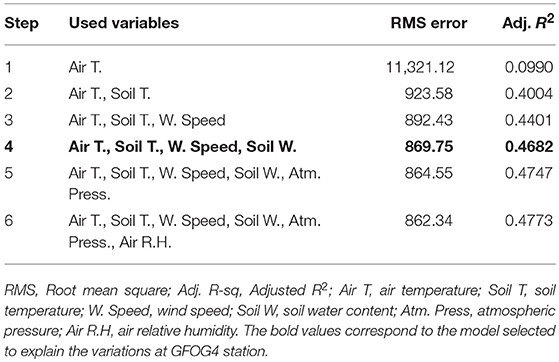
Table 2. Stepwise regression model steps for GFOG4 data (period 2013–2014).

Equation (7) represents the proposed final regression model for the soil CO₂ flux (y), which is composed by the air temperature (Air T.), soil temperature (Soil T.), soil water content (Soil W.) and wind speed (W. Speed):

Soil temperature and wind speed have an inverse influence on the soil CO₂ flux, and for the other side air temperature and soil water content correlate positively.

According to the adjusted R², the model explains around 47% (0.4682) of the gas flux variations in this monitoring site, and soil temperature is the variable with higher explanatory power (about 30% of the CO₂ flux variation).

Based on the model, the predicted and residuals time series were calculated (Figure 4). The predicted values (y) correspond to the estimated values according to the proposed model and for the recent years there is a good agreement between the measured soil CO₂ fluxes and the predicted by the regression (Pearson correlation of 83%).

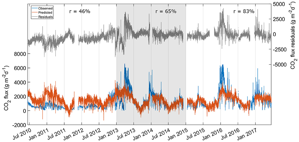
Figure 4. Observed, predicted and residuals soil CO₂ flux time series for GFOG4 station. Pearson correlation coefficients (r) between predicted and observed values are displayed for the different periods. Gray area represents the period used to define the regression model.

Based on Equation (7), predicted values were calculated and the difference between observed and predicted allows to calculate a third time series, the residuals (Figure 4), which correspond to the gas flux variations that cannot be explained by the proposed regression model.

Searching for Cycles

To evaluate the presence of harmonic oscillations a wavelet analysis and a spectral analysis were performed to the time series. The spectrogram was calculated using 512 samples of the time series with a step of 24 samples and to minimize spectral leakage, a Hanning window was used, similarly to previous studies. Considering that the sample rate is 24 samples per day in the studied time series, the Nyquist critical frequency will be 12 cycles per day. Based on results obtained in previous works, more than 2 or 3 cycles per day should not be expected, which shows that this sample rate is adequate for this study.

Figure 5 shows the results of the FFT and wavelet analyses performed on the soil CO₂ fluxes and residuals for the period used to perform the models. One cycle per day (cpd), corresponding to the diurnal peak (S₁), may be observed on both the spectrogram (FFT analysis, Figures 5A,C) and on the scalogram (wavelet analysis, Figure 5B), even if 1 cpd signal is not constant along the time series and shows different intensities. The higher noise observed on the spectrogram close to the origin (Figure 5A) compared with the scalogram can be explained as the DFT normally represents the zero frequency as the offset from the time series to the origin.

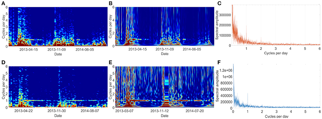
Figure 5. Spectral results for the observed and residuals soil CO₂ fluxes for the period 2013–2014: (A) spectrogram, (B) scalogram and (C) FFT spectrum of the observed values; (D) spectrogram, (E) scalogram (F) and FFT spectrum of the residuals.

The spectrum of the soil CO₂ fluxes shows however 1 and 2 cpd (Figure 5C); the weaker 2 cpd (12 h cycle) does not appear in the spectrogram or even in the scalogram. FFT and wavelet analyses were also applied to the environmental time series (Supplementary Figure 1) in order to identify the periodic behavior, as well as, to highlight eventual differences using both methodologies (Table 3). Higher number of cycles were identified based on the spectrograms when compared with the scalograms, namely for the atmospheric pressure, air and soil temperature.

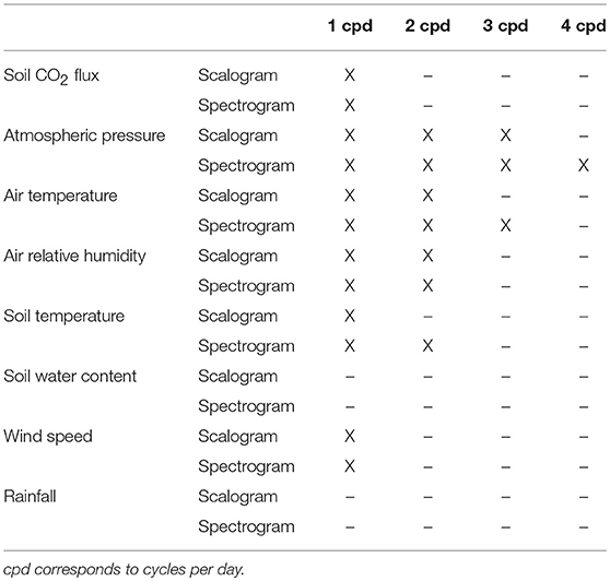
Table 3. Identified daily cycles for the different monitored variables based on the two spectral methodologies.

FFT spectrum applied to the entire monitored period shows higher energy peaks at a periodicity of 358 day, which coincide in general with the annual cycle (Figure 6).

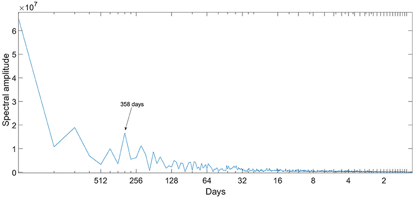
Figure 6. Amplitude spectrum showing the low-frequency peaks for the entire monitored period of the observed soil CO₂ fluxes.

Spectral analysis was also applied to the residuals in order to check if the filtered time series still shows harmonic behavior. Figures 5D–F show that 1 cpd is also found out in this time series, even if the 2 cpd is practically absent on the spectrum. Considering that high frequency cycles are still observed on the residuals time series, a second order of filtering was applied to the residuals dataset, namely a Butterworth filter (Figure 7). The greenish band in Figure 7 represents the mean plus-minus two times the standard deviation of the filtered residuals ($\overline{y}\pm 2\sigma$) estimated for the period 2013–2014.

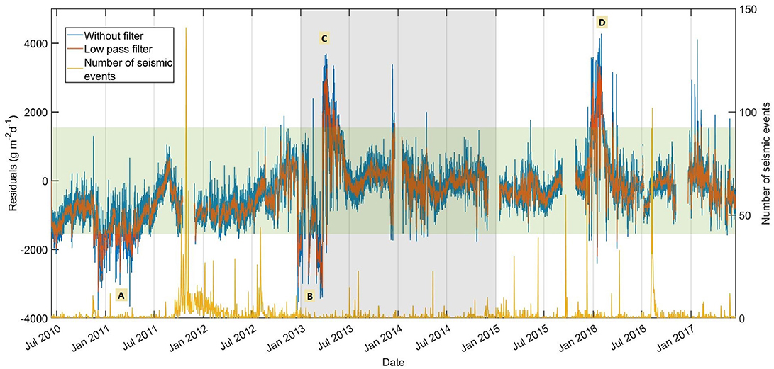
Figure 7. Soil CO₂ flux residuals at GFOG4 station after applying the two step filtering (MRA and Butterworth filters). Orange line corresponds to the number of seismic events recorded at Fogo Volcano (CIVISA catalog). Gray vertical band represents the period used to produce the regression model and the green band corresponds to the interval ($\overline{y}\pm 2\sigma$).

Discussion

GFOG4 station is installed in an anomalous soil CO₂ flux and temperature area, and is clearly located in a Diffuse Degassing Structure (DDS, Chiodini et al., 2001) in the north flank of Fogo Volcano (S. Miguel Island). This monitoring site corresponds to the one that shows the highest average soil CO₂ flux emissions (1,165 gm⁻²d⁻¹) from all the permanent stations installed at S. Miguel Island (Viveiros et al., 2008, 2015a).

As previously mentioned, multivariate regression analysis has been commonly applied to gas geochemical time series in different degassing areas (e.g., Granieri et al., 2003, 2010; Padrón et al., 2008; Viveiros et al., 2008; Laiolo et al., 2012, 2016; Neri et al., 2016; Lelli and Raco, 2017) and showed to be adequate to highlight and filter the influences of the environmental parameters on the gas flux. The stepwise regression model here suggested as filtering methodology was already applied to other CO₂ and ²²²Rn time series in the Azores archipelago (Silva et al., 2015; Viveiros et al., 2015a) and, despite all the advantages already mentioned for the linear regression analysis, the stepwise multivariate regression analysis also facilitates the selection of the independent variables to be included in the model, as well as, it is automatic and less user dependent. The model here proposed explains about 47% of the gas flux variations at GFOG4 site and the Pearson correlation coefficients between the observed and the predicted time series for the period between 2015 and 2017 is 0.83, which suggests a good agreement between both time series and the adequacy of the model to explain the observed CO₂ flux variations. The Pearson correlation coefficient for the period from 2010 to 2013 was significantly lower (0.46). This distinct behavior can be eventually justified by the initial period of instability of the expanded degassing area. In fact, previous studies (Viveiros et al., 2015a) already highlighted that the installation procedure of a permanent station can interfere with the initial acquired datasets, as it can cause higher variability on the gas flux data recorded.

The stepwise multivariate regression model proposed for the data between 2013 and 2014 shows that the soil temperature is the variable with greater influence on the soil CO₂ fluxes explaining about 30% of the gas variations (Table 2). Similar inverse correlation between soil CO₂ fluxes and soil temperature was already highlighted in other permanent soil CO₂ flux stations installed at Furnas and Fogo volcanoes (S. Miguel Island) (Viveiros et al., 2008, 2015a), or even in other degassing areas, such as Stromboli Volcano (Laiolo et al., 2016). Viveiros et al. (2008) suggested that these inverse correlations should result from the long-term seasonal effects, with the lower emissions occurring during summer time when compared with the winter period. Similar seasonal behavior is observed at GFOG4 site (Figure 1) and the seasonal cycle was identified (Figure 6).

Wind speed also correlates inversely with the soil CO₂ fluxes at GFOG4 station and this influence is in agreement with previous observations in other monitoring sites of S. Miguel Island (GFUR2, GFUR3, GFOG3, and GFOG3.1 stations). Intrusion of some air into the upper parts of the soil may dilute the soil gases and decrease the CO₂ fluxes during high wind speed periods. Air temperature and soil water content correlate positively with the soil gas flux according to the regression model proposed (Equation 7). The positive correlation between soil water content and gas fluxes was also previously identified in other monitoring sites and it was explained by the covering effect of the station shelter that maintains the soil dry during rainfall periods and allows the gas to escape. In the area surrounding the permanent stations the soil is wet and the pores are saturated, fact that hinders gas release. Several spike-like anomalies observed on the soil CO₂ fluxes time series are associated with the increases on the soil water content. This type of association was observed not only on the Azores monitoring sites (Viveiros et al., 2008, 2009, 2015a) but also on other sites with similar monitoring stations, such as at the summit area of Usu (Mori et al., 2002), Solfatara (Granieri et al., 2003, 2010) and Stromboli volcanoes (Carapezza et al., 2009). The positive correlation between air temperature and soil CO₂ flux is not widely observed and usually both variables correlate inversely as the CO₂ fluxes depend on the daily thermal cycles (Rinaldi et al., 2012; Viveiros et al., 2014). However, this positive correlation has been also identified at GFOG3.1 station and it was explained as resulting from an artifact, i.e., the superimposition of other monitored environmental variables. One additional explanation is that both monitoring sites are located in a thermally anomalous zone, that can eventually unbalance the expected pressure gradients on the soil-air interface due to the thermal cycles. In fact, and even if the models are specific for each monitoring site, considering that different characteristics (e.g., soil properties, drainage area, topography) can control the effect that environmental variables have on the soil CO₂ fluxes (Viveiros et al., 2008, 2014), the model here proposed is quite similar to the regression defined to GFOG3.1 station. In this case, with exception to the atmospheric pressure, the same environmental variables correlate with the CO₂ fluxes and show similar type of influence (for more details on GFOG3.1 station see Viveiros et al., 2015a).

Considering that previous studies applied to volcanic gas emissions used both Fast Fourier Transform and wavelet analyses as the spectral techniques, we applied both techniques to the soil CO₂ flux time series in order to evaluate potential differences and discuss their adequacy to apply in a real-time monitoring system. Spectral analyses applied to the soil CO₂ flux time series identified the diurnal (S₁) peak (Figure 5), even if only the FFT spectra recognized a weaker semidiurnal cycle (12 h variation). Similar diurnal cycles were also recognized in the CO₂ flux time series not only in the Azores archipelago (Rinaldi et al., 2012; Viveiros et al., 2014), but also in other soil diffuse degassing areas (Granieri et al., 2003; Padrón et al., 2008; Hernández et al., 2012) and were mainly explained and modeled as consequence of the influence of the meteorological variables (Rinaldi et al., 2012; Viveiros et al., 2014). A low frequency signal (period of 358 days), which represents the annual period, was recognized on the spectrum soil CO₂ fluxes for the whole period. A cycle of about 340 days was previously identified at Furnas Volcano permanent stations (Viveiros et al., 2014) and it was interpreted as representing the annual period. The divergence to the 365 days was then interpreted as a FFT resolution problem caused by the length of the analyzed time series. In fact, in the current study with 7 years of data available, the identified annual cycle (358 days) approaches the annual band when compared with the results obtained by Viveiros et al. (2014).

This study used two different spectral approaches, which were previously applied to volcanic gas data, to the recorded time series in order to discriminate potential differences and evaluate which approach could be more adequate for a real-time monitoring environment. Even if both techniques identified the diurnal cycle on the soil CO₂ flux time series and showed quite similar behavior in the spectrogram and in the scalogram (Figure 5), by definition wavelet analysis should be more permissible to the lack of data, what can be advantageous to use for monitoring time series that frequently are affected by technical problems. Other positive aspect of the use of wavelets should be a better detection of the cycle (stability of the periodicities). These differences were not however particularly evident in the current study. In addition to the fact that it is easier to apply, FFT also allows to calculate the spectra and consequently allows to identify low frequencies. The soil CO₂ flux spectra (Figure 5C) also showed the semidiurnal cycle, which was not highlighted in the spectrogram or in the scalogram. One potential explanation may be that this weaker signal was hidden in the noise, especially in the winter periods, when the time series is more scattered. The existence of periodicities in the other monitored environmental variables was also evaluated (Table 3) and FFT again better discriminates high frequencies when compared with the wavelet analyses. Some of these high frequencies may eventually be due to harmonics of the diurnal signal, however looking at the other side one may suggest that wavelets hide some of the frequencies.

Considering the recognized periodicities in the environmental variables and the fact that the semidiurnal cycle is still detected in the residuals time series (Figures 5D–F), and even if there is a good agreement between the observed and predicted values, the regression model proposed does not seem to filter all the external influences on the soil CO₂ fluxes. Viveiros et al. (2014) also identified this problem in the time series recorded at Furnas Volcano (S. Miguel Island) and suggested a second filtering procedure using the FFT low-pass filter. In the current study we suggest the use of the Butterworth filter as it reduces the computational tasks and requires a lower number of samples to be considered for filtering, which is more appropriate for a real-time monitoring system.

The final calculated residuals dataset (Figure 7), resulting from two step filtering, should be the one used in any Volcano Observatory as the best representative of the deep-source gas flux variations. Similarly to previous studies (Viveiros et al., 2014, 2015a), a band of variation was defined and any values that lay outside this band can represent anomalous periods of activity and need to be evaluated as a multidisciplinary approach since they may represent precursors of deep changes in the system. Four main periods in Figures 7 (A, B, C and D) were highlighted and, even if the main scope of the current study was to apply different statistical methodologies to the soil gas flux time series and evaluate its adequacy for automation in a real-time monitoring basis, an attempt to correlate the gas flux residuals with the number of seismic events recorded at Fogo Volcano was done. No direct correlation was observed between the identified anomalous periods for the residuals and the number of seismic events. Periods identified as “B” and “C” are probably a local response of the system to some works carried out by the geothermal company in the area surrounding the station and that included injection of concrete at depth. These works were developed between July 2012 and March 2013, thus coincident with the above mentioned anomalous periods. As mentioned previously, the installation of a permanent station may also drive some period of instability in the gas release and this can potentially be the explanation to the lower than expected CO₂ fluxes at period “A”. Even if anomalous period “D” (between end of December 2015 and early February 2016) occurs after a seismic swarm with 71 events, other similar seismic swarms did not cause significant changes on the CO₂ fluxes. A common observation for all the anomalous periods is that they occur during winter periods, when the gas flux data are more scattered and thus more challenging for the statistical approaches applied. GPS data are only available in the literature for the period from 2010 to May 2013 (Okada et al., 2015). Those authors highlighted deformation on the Fogo Volcano edifice for the period September 2011 to August 2012, associated with some of the recorded seismic swarms. The CO₂ flux residuals do not show any anomalous values for that period, but the anomalous vectors are mainly in the eastern part of the volcano edifice and not close to the GFOG4 monitoring site.

Conclusions

Environmental variables explain almost half of the variation observed on the soil CO₂ fluxes recorded in this monitoring site. This relevant correlation between gas fluxes and external factors was already shown in several degassing areas worldwide and, for this reason, it is fundamental to filter the data in order to highlight variations that may represent the deep volcanic/hydrothermal processes. In what concerns the statistical approaches applied, both spectral analyses seem adequate to apply to the soil CO₂ time series. However, considering that the wavelets are more complex to apply and may even hide eventual frequencies, we suggest the coupled use of stepwise multivariate regression analyses and FFT analyses as a good approach to filter external influences from the soil gas fluxes. The second order filtering, when high frequencies on the residuals are identified, may be carried out using the Butterworth filter since it is easy to apply in a routine time-real monitoring environment.

In the particular case of GFOG4 site, the final residuals do not show trends, nor any persistent increase that could eventually be correlated with some unrest, nor a decrease that could show a reduction of the anomaly in an area that expanded after a geothermal drilling. This observation seems to highlight that a constant and persistent deep flux of gas is being released in this degassing area. Nevertheless, analyses of the residuals show some periods laying outside the “normal” band and four anomalous periods were identified, but no direct correlation with the seismic and/or ground deformation observed at Fogo Volcano was established. We have to consider the low magnitude of the earthquakes and the fact that the ground deformation was identified in a different sector of the volcano edifice. Future studies should develop additional tools to join multidisciplinary time series recorded in the volcano observatories. A closer look to these variations shows that these periods occur essentially in the winter when the time series are more scattered and potentially represent periods of extreme weather conditions that the regression model does not manage to account.

The definition of intervals of variation considered “normal” are crucial to identify the anomalous periods especially in any Volcano Observatory, where recognizing precursors of volcanic activity is challenging and demanding. The application of automatic methods is a relevant approach that allows any user to identify potential anomalies. In addition to what mentioned above and considering the effect that environmental changes may have also on other gas species, such as radon (e.g., Perrier and Girault, 2013; Silva et al., 2015), the methodologies now proposed can be also tested and expanded to other degassing series and used as routine in any Volcano Observatory. Each Volcano Observatory should build specific models for the different monitoring sites. However, the use of the two steps filtering, coupling regression and spectral methodologies, will improve not only the knowledge about the gas flux behavior but also will allow to easily detect anomalous degassing periods.

Author Contributions

SO and FV processed the data and mainly wrote the manuscript. CS and JP provided important suggestions during the processing and discussion of the data. All the authors have read and approved the final manuscript.

Conflict of Interest Statement

The authors declare that the research was conducted in the absence of any commercial or financial relationships that could be construed as a potential conflict of interest.

Acknowledgments

The present study was developed with the support of VOLRISKMAC, INTERREG MAC 2014–2020 (MAC/3.5b/124). Authors would like to thank CIVISA to allow the use of the seismic data catalog. The first version of the manuscript was also improved with the contribution of the two reviewers and the editor.

Supplementary Material

The Supplementary Material for this article can be found online at: https://www.frontiersin.org/articles/10.3389/feart.2018.00208/full#supplementary-material

References

Aiuppa, A., Burton, M., Caltabiano, T., Giudice, G., Gurrieri, S., Liuzzo, M., et al. (2010). Unusually large magmatic CO2 gas emissions prior to a basaltic paroxysm. Geophys. Res. Lett. 37:L17303. doi: 10.1029/2010GL043837
Allard, P., Carbonnelle, J., Dajlevic, D., Le Bronec, J., Morel, P., Robe, M. C., et al. (1991). Eruptive and diffuse emissions of CO2 from Mount Etna. Nature 351, 387–391.
Baubron, J. C., Allard, P., and Toutain, J. P. (1990). Diffuse volcanic emissions of carbon dioxide from Vulcano Island, Italy. Nature 344, 51–53.
Boichu, M., Oppenheimer, C., Tsanev, V., and Kyle, P. (2010). High temporal resolution SO2 flux, measurements at Erebus volcano, Antarctica. J. Volcanol. Geotherm. Res. 190, 325–336. doi: 10.1016/j.jvolgeores.2009.11.020
Brusca, L., Inguaggiato, S., Longo, M., Madonia, P., and Maugeri, R. (2004). The 2002–2003 eruption of Stromboli (Italy): Evaluation of the volcanic activity by means of continuous monitoring of soil temperature, CO2 flux, and meteorological parameters. Geochem. Geophys. Geosyst. 5:Q12001. doi: 10.1029/2004GC000732
Caliro, S., Viveiros, F., Chiodini, G., and Ferreira, T. (2015). Gas geochemistry of hydrothermal fluids of the S. Miguel and Terceira Islands, Azores. Geochim. Cosmochim. Acta 168, 43–57. doi: 10.1016/j.gca.2015.07.009
Cannata, A., Giudice, G., Gurrieri, S., Montalto, P., Alparone, S., Di Grazia, G., et al. (2010). Relationship between soil CO2 flux and volcanic tremor at Mt. Etna: Implications for magma dynamics. Environ. Earth. Sci. 61, 477–489. doi: 10.1007/s12665-009-0359-z
Carapezza, M. L., Inguaggiato, S., Brusca, L., and Longo, M. (2004). Geochemical precursors of the activity of an open-conduit volcano: the Stromboli 2002–2003 eruptive events. Geophys. Res. Lett. 31:L07620. doi: 10.1029/2004GL019614
Carapezza, M. L., Ricci, T., Ranaldi, M., and Tarchini, L. (2009). Active degassing structures of Stromboli and variations in diffuse CO2 output related to the volcanic activity. J. Volcanol. Geotherm. Res. 182, 231–245. doi: 10.1016/j.jvolgeores.2008.08.006
Carmo, R., Madeira, J., Ferreira, T., Queiroz, G., and Hipólito, A. (2015). “Volcano-tectonic structures of S. Miguel Island, Azores,” in Volcanic Geology of S. Miguel Island (Azores archipelago), eds J. L. Gaspar, J. E. Guest, A. M. Duncan, F. J. A. S. Barriga, and D. K. Chester (London: Geological Society, London, Memoirs), 65–86. doi: 10.1144/M44.6
Chiodini, G., Cioni, R., Guidi, M., Raco, B., and Marini, L. (1998). Soil CO2 flux measurements in volcanic and geothermal areas. Appl. Geochem. 13, 543–552.
Chiodini, G., Frondini, F., Cardellini, C., Granieri, D., Marini, L., and Ventura, G. (2001). CO2 degassing and energy release at Solfatara Volcano, Campi Flegrei, Italy. J. Geophys. Res. 106, 16213–16221. doi: 10.1029/2001JB000246
Cooley, W., and Tukey, J. W. (1965). An algorithm for the machine calculation of complex fourier series. Math. Comput. 19, 297–301.
Draper, N., and Smith, H. (1981). Applied Regression Analysis, 2nd Edn. New York, NY: John Wiley & Sons, Inc.
Farge, M. (1992). Wavelet transforms and their applications to turbulence. Annu. Rev. Fluid Mech. 24, 395–457.
Ferreira, T., Gaspar, J. L., Viveiros, F., Marcos, M., Faria, C., and Sousa, F. (2005). Monitoring of fumarole discharge and CO2 soil degassing in the Azores: contribution to volcanic surveillance and public health risk assessment. Ann. Geophys. 48, 787–796. doi: 10.4401/ag-3234
Fischer, T. P., and Chiodini, G. (2015). “Volcanic, Magmatic and Hydrothermal Gases,” in The Encyclopedia of Volcanoes, 2nd Ed., eds H. Sigurdsson, B. Houghton, S. R. McNutt, H. Rymer, and J. Stix (San Diego, CL: Elsevier Inc.), 779–797.
Granieri, D., Avino, R., and Chiodini, G. (2010). Carbon dioxide diffuse emission from the soil: ten years of observations at Vesuvio and Campi Flegrei (Pozzuoli), and linkages with volcanic activity. Bull. Volcanol. 72, 103–118. doi: 10.1007/s00445-009-0304-8
Granieri, D., Chiodini, G., Marzocchi, W., and Avino, R. (2003). Continuous monitoring of CO2 soil diffuse degassing at Phlegraean Fields (Italy): influence of environmental and volcanic parameters. Earth Planet. Sci. Lett. 212, 167–179. doi: 10.1016/S0012-821X(03)00232-2
Grossmann, A., and Morlet, J. (1984). Decomposition of Hardy functions into square integrable wavelets of constant shape. SIAM J. Math. Anal. 15, 723–736. doi: 10.1137/0515056
Gurrieri, S., Liuzzo, M., and Giudice, G. (2008). Continuous monitoring of soil CO2 flux on Mt. Etna: The 2004–2005 eruption and the role of regional tectonics and volcano tectonics, J. Geophys. Res. 113:B09206. doi: 10.1029/2007JB005003
Hernández, P. A., Padilla, G., Padrón, E., Pérez, N. M., Calvo, D., Nolasco, D., et al. (2012). Analysis of long- and short-term temporal variations of the diffuse CO2 emission from Timanfaya volcano, Lanzarote, Canary Islands. Appl. Geochem. 27, 2486–2499. doi: 10.1016/j.apgeochem.2012.08.008
Inguaggiato, S., Vita, F., Cangemi, M., Mazot, A., Sollami, A., Calderone, L. M. P., et al. (2017). Stromboli volcanic activity variations inferred from observations of fluid geochemistry: 16 years of continuous monitoring of soil CO2 fluxes (2000–2015). Chem. Geol. 469, 69–84. doi: 10.1016/j.chemgeo.2017.01.030
Jurišić, D., Moschytz, G. S., and Mijat, N. (2002). “Single Amplifier, Active-RC, Butterworth, and Chebyshev Filters Using Impedance Tapering,” in Proceedings of the IASTED International Conference: Signal Processing, Pattern Recognition & Applictions (Creta).
Laiolo, M., Cigolini, C., Coppola, D., and Piscopo, D. (2012). Developments in real-time radon monitoring at Stromboli volcano. J. Environ. Radioact. 105, 21–29. doi: 10.1016/j.jenvrad.2011.10.006
Laiolo, M., Ranaldi, M., Tarchini, L., Carapezza, M. L., Coppola, D., Ricci, T., et al. (2016). The effects of environmental parameters on diffuse degassing at Stromboli volcano: Insights from joint monitoring of soil CO2 flux and radon activity. J. Volcanol. Geotherm. Res. 315, 65–78. doi: 10.1016/j.jvolgeores.2016.02.004
Lelli, M., and Raco, B. (2017). A reliable and effective methodology to monitor CO2 flux from soil: the case of Lipari Island (Sicily, Italy). Appl. Geochem. 85, 73–85. doi: 10.1016/j.apgeochem.2017.08.004
Liuzzo, M., Gurrieri, S., Giudice, G., and Giuffrida, G. (2013). Ten years of soil CO2 continuous monitoring on Mt. Etna: exploring the relationship between processes of soil degassing and volcanic activity. Geochem. Geophys. Geosyst. 14, 2886–2899. doi: 10.1002/ggge.20196
Mallat, S. (2009). A Wavelet Tour of Signal Processing, The Sparse Way. Burlington, MA: Academic Press.
Meignen, S., Oberlin, T., and McLaughlin, S. (2012). A new algorithm for synchrosqueezing: with an application to multicomponent signals sampling and denoising. IEEE Trans. Signal Proces. 60, 5787–5798. doi: 10.1109/TSP.2012.2212891
Mori, T., Notsu, K., Hernández, P. A., Salazar, J. M. L., Pèrez, N., Virgili, G., et al. (2002). Continuous monitoring of soil CO2 efflux from the summit region of Usu Volcano, Japan. Bull. Volcanol. Soc. Japan 47, 339–345.
Muecke, G. K., Ade-Hall, J. M., Aumento, F., Macdonald, A., Reynolds, P. H., Hyndman, R. D., et al. (1974). Deep drilling in an active geothermal area in the Azores. Nature 252, 281–285.
Neri, M., Ferrera, E., Giammanco, S., Currenti, G., Cirrincione, R., Patan,è, G., et al. (2016). Soil radon measurements as a potencial tracer of tectonic and volcanic activity. Sci. Rep. 6:24581. doi: 10.1038/srep24581
Neter, J., Wasserman, W., and Kunter, M. H. (1983). Applied Linear Regression Models. Homewood: Richard D. Irwin, Inc.
Okada, J., Sigmundsson, F., Ófeigsson, B., Ferreira, T., and Rodrigues, R. (2015). “Tectonic and volcanic deformation at São Miguel Island, Azores, observed by continuous GPS analysis 2008-13,” in Volcanic Geology of S. Miguel Island (Azores archipelago), eds J. L. Gaspar, J. E. Guest, A. M. Duncan, F. J. A. S. Barriga, and D. K. Chester (London: Geological Society, London, Memoirs), 239–256.
Padrón, E., Melián, G., Marrero, R., Nolasco, D., Barrancos, J., Padilla, G., et al. (2008). Changes in the diffuse CO2 emission and relation to seismic activity in and around El Hierro, Canary Islands. Pure Appl. Geophys. 165, 95–114. doi: 10.1007/s00024-007-0281-9
Pardoe, I., Simon, L., and Young, D. (2018). Lesson 5: Multiple Linear Regression. Available online at: https://onlinecourses.science.psu.edu/stat501/node/283
Pérez, N. M., Hernández, P. A., Padrón, E., Cartagena, R., Olmos, R., Barahona, F., et al. (2006). Anomalous diffuse CO2 emission prior to the January 2002 short-term unrest at San Miguel Volcano, El Salvador, Central America. Pure Appl. Geophys. 163, 883–896. doi: 10.1007/s00024-006-0050-1
Pérez, N. M., Padilla, G. D., Padrón, E., Hernández, P. A., Melián, G. V., Barrancos, J., et al. (2012). Precursory diffuse CO2 and H2S emission signatures of the 2011–2012 El Hierro submarine eruption, Canary Islands. Geophys. Res. Lett. 39;L16311. doi: 10.1029/2012GL052410
Pering, T. D., Tamburello, G., McGonigle, A. J. S., Aiuppa, A., Cannata, A., Giudice, G., et al. (2014). High time resolution fluctuations in volcanic carbon dioxide degassing from Mount Etna. J. Volcanol. Geotherm. Res. 270, 115–121. doi: 10.1016/j.jvolgeores.2013.11.014
Perrier, F., and Girault, F. (2013). Harmonic response of soil radon-222 flux and concentration induced by barometric oscillations. Geophys. J. Int. 195, 945–971. doi: 10.1093/gji/ggt280
Press, W. H., Teukolsky, S. A., Vetterling, W. T., and Flannery, B. P. (1992). Numerical Recipes in C: The Art of Scientific Computing. New York, NY: Cambridge University Press.
Rawlings, J. O., Pantula, S. G., and Dickey, D. A. (1998). Applied Regression Analysis: A Research Tool, 2nd Edn. New York, NY: Springer-Verlag.
Rinaldi, A. P., Vandemeulebrouck, J., Todesco, M., and Viveiros, F. (2012). Effects of atmospheric conditions on surface diffuse degassing. J. Geophys. Res. 117:B11201. doi: 10.1029/2012JB009490
Salazar, J. M. L., Hernández, P. A., Pérez, N. M., Olmos, R., Barahona, F., Cartagena, R., et al. (2004). Spatial and temporal variations of diffuse CO2 degassing at the Santa Ana-Izalco-Coatepeque volcanic complex, El Salvador, Central America. Geol. Soc. Am. Spec. Pap. 375, 135–146. doi: 10.1130/0-8137-2375-2.135
Salazar, J. M. L., Pérez, N. M., Hernández, P. A., Soriano, T., Barahona, F., Olmos, R., et al. (2002). Precursory diffuse carbon dioxide degassing signature related to a 5.1 magnitude earthquake in El Salvador, Central America. Earth Planet. Sci. Lett. 205, 81–89. doi: 10.1016/S0012-821X(02)01014-2
Sedra, A., and Smith, K. (2004). Microelectronic Circuits, 5th Edn. Oxford, NY: Oxford University Press.
Shu, W., and Qinyu, L. (2005). Some Problems on the Global Wavelet Spectrum. J. Ocean Univ. China 4, 398–402. doi: 10.1007/s11802-005-0062-y
Silva, C., Viveiros, F., Ferreira, T., Gaspar, J. L., and Allard, P. (2015). “Diffuse soil emanations of radon and hazard implications at Furnas Volcano, São Miguel Island (Azores),” in Volcanic Geology of S. Miguel Island (Azores archipelago), eds J. L. Gaspar, J. E. Guest, A. M. Duncan, F. J. A. S. Barriga, and D. K. Chester (London: Geological Society, London, Memoirs), 197–211.
Silva, R. (2011). Evaluation of Spatial and Temporal Seismicity Patterns in the Central Region of São Miguel (Azores): Implications for Whole-Island Seismic Hazard Assessment. PhD Thesis, University of the Azores, 236.
Silva, R., Havskov, J., Bean, C., and Wallenstein, N. (2012). Seismic swarms, fault plane solutions and stress tensors for São Miguel Island central region (Azores). J. Seismol. 16, 389–407. doi: 10.1007/s10950-012-9275-x
Torrence, C., and Compo, G. (1998). A practical guide to wavelet analysis. B. Am. Meteorol. Soc. 79, 61–78.
Viveiros, F., Ferreira, T., Cabral Vieira, J., Silva, C., and Gaspar, J. L. (2008). Environmental influences on soil CO2 degassing at Furnas and Fogo volcanoes (São Miguel Island, Azores archipelago). J. Volcanol. Geotherm. Res. 177, 883–893. doi: 10.1016/j.jvolgeores.2008.07.005
Viveiros, F., Ferreira, T., Silva, C., and Gaspar, J. L. (2009). Meteorological factors controlling soil gases and indoor CO2 concentration: a permanent risk in degassing areas. Sci. Tot. Environ. 407, 1362–1372. doi: 10.1016/j.scitotenv.2008.10.009
Viveiros, F., Ferreira, T., Silva, C., Vieira, J. C., Gaspar, J. L., Virgili, G., et al. (2015a). “Permanent monitoring of soil CO2 degassing at Furnas and Fogo volcanoes (São Miguel Island, Azores),” in Volcanic Geology of S. Miguel Island (Azores archipelago), eds J. L. Gaspar, J. E. Guest, A. M. Duncan, F. J. A. S. Barriga, and D. K. Chester (London: Geological Society, London, Memoirs), 271–288.
Viveiros, F., Gaspar, J. L., Ferreira, T., and Silva, C. (2016). Hazardous indoor CO2 concentrations in volcanic environments. Environ. Pollut. 214, 776–786. doi: 10.1016/j.envpol.2016.04.086
Viveiros, F., Gaspar, J. L., Ferreira, T., Silva, C., Marcos, M., and Hipólito, A. (2015b). “Mapping of soil CO2 diffuse degassing at São Miguel Island and its public health implications,” in Volcanic Geology of S. Miguel Island (Azores archipelago), eds J. L. Gaspar, J. E. Guest, A. M. Duncan, F. J. A. S. Barriga, and D. K. Chester (London: Geological Society, London, Memoirs), 185–195.
Viveiros, F., Vandemeulebrouck, J., Rinaldi, A. P., Ferreira, T., Silva, C., and Cruz, J. V. (2014). Periodic behavior of soil CO2 emissions in diffuse degassing areas of the Azores archipelago: application to seismovolcanic monitoring. J. Geophys. Res. 119, 7578–7597. doi: 10.1002/2014JB011118
Wallenstein, N., Duncan, A. M., Guest, J. E., and Almeida, M. H. (2015). “Eruptive history of Fogo Volcano, São Miguel, Azores,” in Volcanic Geology of S. Miguel Island (Azores archipelago), eds J. L. Gaspar, J. E. Guest, A. M. Duncan, F. J. A. S. Barriga, and D. K. Chester (London: Geological Society, London, Memoirs), 105–123.
Keywords: soil CO2 flux time series, stepwise multivariate regression analysis, Fast Fourier Transform, wavelets, seismo-volcanic monitoring
Citation: Oliveira S, Viveiros F, Silva C and Pacheco JE (2018) Automatic Filtering of Soil CO2 Flux Data; Different Statistical Approaches Applied to Long Time Series. Front. Earth Sci. 6:208. doi: 10.3389/feart.2018.00208
Received: 30 July 2018; Accepted: 31 October 2018;
Published: 20 November 2018.
Edited by:
Valerio Acocella, Università degli Studi Roma Tre, ItalyReviewed by:
Agnes Mazot, GNS Science, New ZealandMicol Todesco, Istituto Nazionale di Geofisica e Vulcanologia, Italy
Copyright © 2018 Oliveira, Viveiros, Silva and Pacheco. This is an open-access article distributed under the terms of the Creative Commons Attribution License (CC BY). The use, distribution or reproduction in other forums is permitted, provided the original author(s) and the copyright owner(s) are credited and that the original publication in this journal is cited, in accordance with accepted academic practice. No use, distribution or reproduction is permitted which does not comply with these terms.
*Correspondence: Fátima Viveiros, maria.fb.viveiros@azores.gov.pt