Next-Generation Optical Sensing Technologies for Exploring Ocean Worlds—NASA FluidCam, MiDAR, and NeMO-Net
 Ved Chirayath
 Alan Li
- NASA Ames Laboratory for Advanced Sensing, Mountain View, CA, United States
We highlight three emerging NASA optical technologies that enhance our ability to remotely sense, analyze, and explore ocean worlds–FluidCam and fluid lensing, MiDAR, and NeMO-Net. Fluid lensing is the first remote sensing technology capable of imaging through ocean waves without distortions in 3D at sub-cm resolutions. Fluid lensing and the purpose-built FluidCam CubeSat instruments have been used to provide refraction-corrected 3D multispectral imagery of shallow marine systems from unmanned aerial vehicles (UAVs). Results from repeat 2013 and 2016 airborne fluid lensing campaigns over coral reefs in American Samoa present a promising new tool for monitoring fine-scale ecological dynamics in shallow aquatic systems tens of square kilometers in area. MiDAR is a recently-patented active multispectral remote sensing and optical communications instrument which evolved from FluidCam. MiDAR is being tested on UAVs and autonomous underwater vehicles (AUVs) to remotely sense living and non-living structures in light-limited and analog planetary science environments. MiDAR illuminates targets with high-intensity narrowband structured optical radiation to measure an object's spectral reflectance while simultaneously transmitting data. MiDAR is capable of remotely sensing reflectance at fine spatial and temporal scales, with a signal-to-noise ratio 10-103 times higher than passive airborne and spaceborne remote sensing systems, enabling high-framerate multispectral sensing across the ultraviolet, visible, and near-infrared spectrum. Preliminary results from a 2018 mission to Guam show encouraging applications of MiDAR to imaging coral from airborne and underwater platforms whilst transmitting data across the air-water interface. Finally, we share NeMO-Net, the Neural Multi-Modal Observation & Training Network for Global Coral Reef Assessment. NeMO-Net is a machine learning technology under development that exploits high-resolution data from FluidCam and MiDAR for augmentation of low-resolution airborne and satellite remote sensing. NeMO-Net is intended to harmonize the growing diversity of 2D and 3D remote sensing with in situ data into a single open-source platform for assessing shallow marine ecosystems globally using active learning for citizen-science based training. Preliminary results from four-class coral classification have an accuracy of 94.4%. Together, these maturing technologies present promising scalable, practical, and cost-efficient innovations that address current observational and technological challenges in optical sensing of marine systems.
Introduction
Our planet's habitability depends on the health and stability of its largest ecosystem, the global ocean. Persistent multispectral optical remote sensing has been instrumental in monitoring and managing Earth's terrestrial ecosystems for land use and land cover change. Through a sustained satellite land imaging program, first implemented over 40 years ago, remote sensing at various spatial resolutions has provided a global view of our changing planet, enabling scientists to assess ecosystem dynamics, biodiversity, natural hazards, and many other applications. Yet, a comparable sustained marine imaging system, capable of detecting changes in marine ecosystems, remains stubbornly out of reach, albeit increasingly relevant in a changing global biosphere predominantly governed by marine systems. Indeed, as of 2018, 100% of the martian and lunar surfaces have been mapped at a spatial resolution of 100 m or finer in visible wavelengths, compared to an estimated 5% of Earth's seafloor.
Observational, technological, operational, and economic issues are the main factors inhibiting global sustained imaging of the marine environment on par with that of terrestrial ecosystems. Observational challenges arise in remote sensing of aquatic systems due to strong optical attenuation in the water column as well as reflection and refraction from ocean waves at the air-water interface. Remote sensing beyond the photic zone, namely deeper than the first 100 m of the water column in clear waters, cannot be addressed in the near future from airborne, and spaceborne platforms. Instead, underwater vehicles are needed to act as the aircraft and satellites of the ocean realm, creating multispectral optical maps as well as topographic maps with acoustic or optical methods. Technological limitations exist for photon-limited passive remote sensing instruments as well as in situ autonomous underwater vehicles (AUVs), which cannot cover the same areas with nearly the same precision as aircraft and spacecraft. Scalable information systems are not well-established to exploit the myriad of data sources available from in situ and remote sensing observations. The standardization and normalization of terrestrial remote sensing practices, georeferencing, and dataset processing algorithms are not directly applicable to marine datasets. Significant difficulties remain in harmonizing multi-modal datasets acquired from acoustic and optical instruments above and below the surface to perform ecosystem assessment. Finally, the significant cost associated with marine data collection exacerbates each of these challenges, often limiting new technologies from being able to scale to global areas due to economic constraints.
In this report we highlight three emerging NASA technologies, primarily supported by NASA's Earth Science Technology Office (ESTO), that attempt to address some of the aforementioned observational, technological, operational, and economic challenges in the context of a vital marine ecosystem–coral reefs. While these developments by no means provide a whole solution to the challenges of understanding our global ocean, they present promising scalable, practical, and cost-efficient ongoing innovations in this field.
Needs and Challenges in Remote Sensing of Aquatic Systems
Aquatic ecosystems, particularly coral reefs, remain quantitatively poorly characterized by low-resolution remote sensing as a result of refractive distortion from ocean waves and optical attenuation. Earth's coastal environments and shallow reef ecosystems comprise an extensive and global life-support system playing a crucial role in regulating our planet's climate and biodiversity as well as protecting our coastal cities and infrastructure from storm events. These highly sensitive ecosystems respond rapidly to changes in land management and climate as indicated by precipitous changes in their morphology, composition, and species makeup. As a result, global observation of coastal environments and determination of the health and extent of coral reefs is a vital earth science measurement, referred to in a decadal survey by the National Research Council (NRC) as a “bellwether of climate change as reef health can often presage changing trends in circulation, ocean acidity and biodiversity (Board, 2007).”
At present marine ecosystems are experiencing one of most significant changes in their history on Earth, triggered by unprecedented anthropogenic pressures, warming seas, ocean acidification, sea level rise, habitat destruction, agricultural runoff, and overharvesting, among other contributing stressors (Bellwood et al., 2004). Compounding our understanding of the impacts of these rapidly-changing pressures is a severe lack of sustained global baseline habitat mapping data and knowledge of reef makeup over regional areas and short timescales with effective spatial resolutions unaffected by sea state conditions, which can introduce refractive errors at the air-water interface (Edinger et al., 2000; Chirayath and Earle, 2016; Storlazzi et al., 2016). Such data are vital to accurately assess and quantify reef ecosystem health for adequate management of these aquatic resources (Bellwood et al., 2004).
Coral reef and shallow marine ecosystem remote sensing can be broken down into measurement and determination of habitat, geomorphology, water properties, bathymetry and currents, and waves (Goodman et al., 2013). Currently, remote sensing is used to examine coral reef ecosystems primarily at meter and km-scale scales through airborne campaigns (e.g., CORAL (PRISM), AVIRIS, DCS) and spaceborne assets (e.g., LandSat, HICO, IKONOS) (Maeder et al., 2002; Andréfouët et al., 2003; Purkis and Pasterkamp, 2004; Corson et al., 2008). Recently, however, it has been shown that low resolution satellite and airborne remote sensing techniques poorly characterize fundamental coral reef health indicators, such as percent living cover and morphology type, at the cm and meter scale (Chirayath and Instrella, accepted). While commercial satellite and airborne remote sensing instruments can achieve effective spatial resolutions (ESR) of 0.3 m over terrestrial targets, ocean waves, and even a flat fluid surface, distort the true location, size, and shape of benthic features. ESR finer than 10 m is within the regime of refractive distortions from ocean waves and requires a remote sensing methodology capable of correcting for these effects. The classification accuracy of coral reefs, for example, is significantly impacted by the ESR of remote sensing instruments. Indeed, current global assessments of coral reef cover and morphology classification based on 10 m-scale satellite data alone can suffer from errors >36% (Figure 1), capable of change detection only on yearly temporal scales and decameter spatial scales, significantly hindering our understanding of patterns, and processes in marine biodiversity.
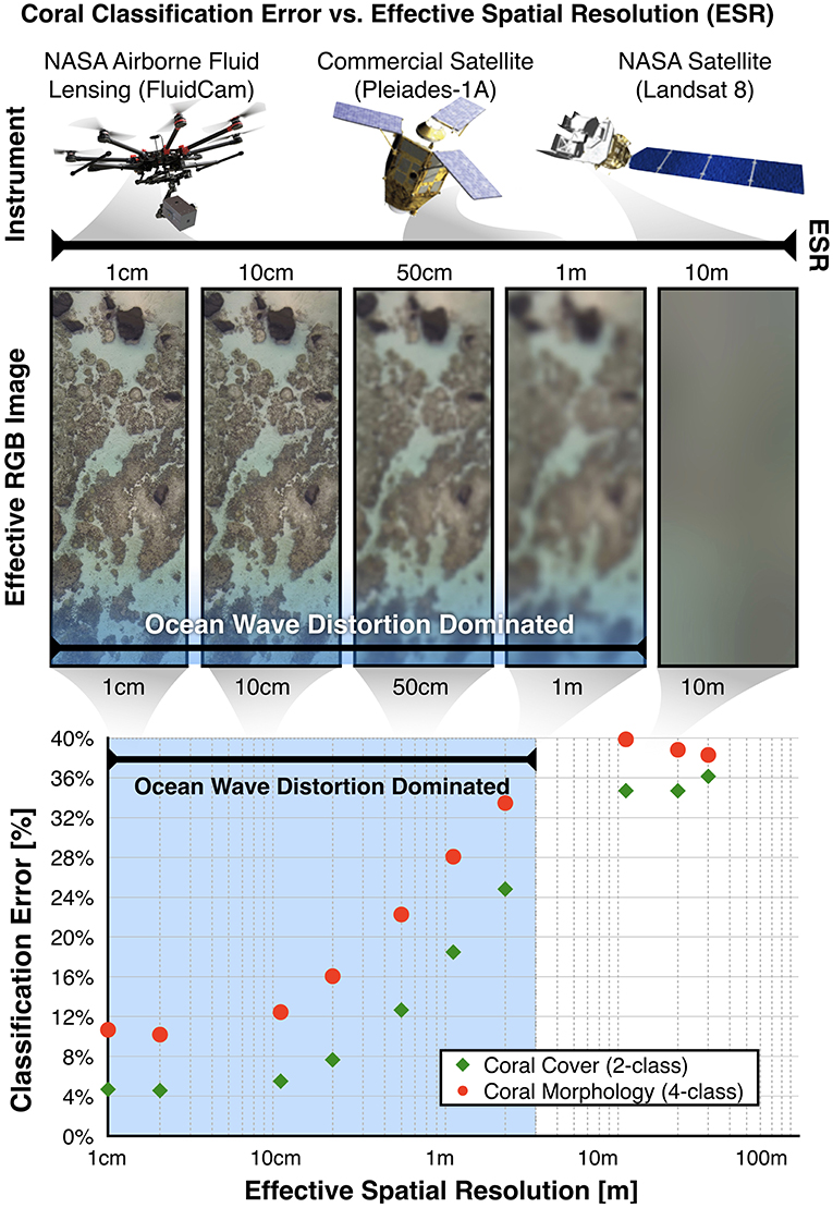
Figure 1. Coral reef classification error as a function of effective spatial resolution (ESR). Using modern machine learning based habitat mapping, coral cover can determined with <5% error at the cm spatial scale with fluid lensing and FluidCam, under a typical range of sea states, 18% error at the 1 m scale from commercial platforms with a perfectly flat sea state, and 34% error at the 10 m scale, typical of sustained land imaging satellites. Adapted with permission from Chirayath and Instrella (accepted).
Even with improved ground sample distance (GSD), state-of-the-art commercial imaging satellites cannot image submerged targets at the same effective spatial resolution (ESR) as terrestrial targets, or consistently georectify benthic surfaces, due to the combined effects of refractive, reflective, and caustic fluid distortions introduced by surface waves (Figure 2) (Chirayath, 2016; Chirayath and Earle, 2016). To address this challenge, we share the NASA FluidCam and fluid lensing technology development, which aims to create a high ESR remote sensing instrument robust to sea state conditions using inexpensive components in a small CubeSat-sized package.
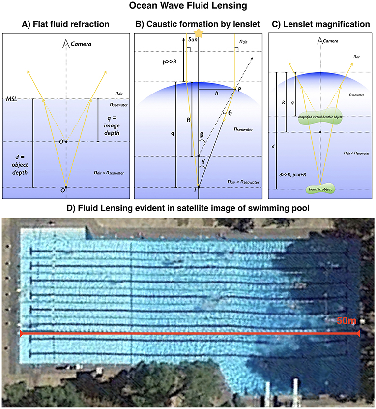
Figure 2. Fluid lensing from ocean waves and its effect on the effective spatial resolution and true location of benthic targets. (A) A calm aquatic surface, when remotely sensed from above, distorts the apparent depth, and spatial position of a benthic target. (B) A curved aquatic surface, or fluid lenslet formed by surface waves, focuses sunlight, forming bright bands of light, or caustics, on the seafloor. (C) A fluid lenslet introduces a net magnification or demagnification effect as a function of curvature. (D) These fluid lensing effects combine to reduce the ESR, SNR, and position of benthic targets. An image captured by state-of-the-art commercial satellite systems, such this 0.3 m GSD Worldview-3 image of an Olympic swimming pool, is noticeably affected by small wave disturbances. Note the distortion of linear lane lines from left to right as a function of surface waves and depth, as well as non-uniform reflectance over pool floor due to caustics. Adapted with permission from Chirayath (2016).
Getting Deeper and Beyond the Photic Zone
Next-generation remote sensing instruments require advances in both passive and active sensing technologies to compare to some of the most sensitive sensors that already exist in the ocean (Tyack, 2000; Madsen et al., 2005). Traditional remote sensing and multispectral imaging of environments from air and space primarily use passive broad-spectrum illumination provided by the Sun coupled with sensitive push broom-style line array photodetectors fitted with narrowband filters to produce multispectral images (Irons et al., 2012). Hyperspectral remote sensing extends this concept further by using photodetectors and scanning spectrometers to resolve hundreds or even thousands of spectral bands (Eismann, 2012). However, in both techniques, atmospheric conditions and the Sun's radiation distribution put limits on which frequencies of light and what SNR are attainable for multispectral imaging on Earth and other planets within our solar system. In aquatic systems, further bounds are introduced as only UV and visible bands of light penetrate the first 100 meters of the clearest waters, the photic zone. As such, current passive multispectral/hyperspectral imagers are limited by ambient conditions along the optical path, ambient illumination spectrum, optical aperture, photodetector SNR, and, consequently, relatively long integration times.
The physical limitations of solar electromagnetic radiation propagation in oceans is one of the chief factors inhibiting the development of a sustained marine imaging program beyond the photic zone. However, significant progress has been made in the past decade with underwater remotely operated or autonomous underwater vehicles (ROVs and AUVs) (Roberts et al., 2010), unmanned surface vehicles (USVs) (Mordy et al., 2017), and profiling floats (Roemmich and Gilson, 2009) to characterize the seafloor, ocean surface, and ocean column over large geographic areas. Recently, three-dimensional photogrammetry, active acoustical methods, and in situ water column measurements have been used with remarkable effectiveness on such platforms to narrow the gap in observational capacity between terrestrial and aquatic systems, revealing mesophotic, and deep sea habitats with unexpected biodiversity and ecological complexity (Pizarro et al., 2004; Bodenmann et al., 2013).
However, the primary means by which global terrestrial ecosystem management has been achieved, through multispectral/hyperspectral remote sensing, is still limited by marine optical instrumentation. Further, relaying data from underwater instruments to and through the surface at bandwidths common to airborne and spaceborne platforms has remained a significant obstacle to sustained deep sea mapping (McGillivary et al., 2018). To address these challenges and extend the depth attainable by airborne remote sensing platforms, we highlight developments behind NASA MiDAR, the Multispectral, Imaging, Detection, and Active Reflectance instrument. MiDAR offers a promising new method for active multispectral in situ and remote sensing of marine systems in previously underutilized spectral bands spanning UV-NIR. As an active optical instrument, MiDAR has the potential to remotely sense deeper than the photic zone defined by the Sun's downwelling irradiance. In addition, MiDAR presents a methodology for simultaneous imaging and optical communications within a fluid and through the air-water interface. Finally, MiDAR makes use of inexpensive narrowband laser and light emitting diodes for the MiDAR transmitter and utilizes the computational imaging capability of the FluidCam instruments for MiDAR receivers.
Making Use of All the Data
With the development of any new instrumentation or measurement capability arise questions of scalability, data management, and interoperability with legacy data and products. How science-driven technology developments scale and address questions pertinent to global marine ecosystems is an ongoing challenge, exacerbated by the ever-increasing volume and complexity of datasets from next-generation instruments. Multispectral 3D data gathered from AUVs, for example, offer high-resolution views of deep-sea systems, but ultimately their scientific value remains limited in scope and application owing to their standalone nature. One sensor may offer a view of a system in certain spectral bands, resolution, and location, while another sensor may gather only topographic data of the same system. Oceanography, in particular, is frequented with such cases of well-understood local systems, captured by independent dedicated field missions, but poorly understood global systems over large time scales. Ultimately, this symptom of marine system sensing is characterized by high spatial and temporal heterogeneity in datasets and low interoperability among multimodal sensing systems.
Fortunately, instrument technology development has occurred alongside advances in information systems technology, capable of handing the growing volume of data and computational overhead. Machine learning for Earth Science applications, in particular, has gained traction, and credibility in recent years as an increasing fleet of commercial and research satellites has driven developments in scaling remote sensing assessment capabilities through semiautonomous and autonomous processing pipelines (Nemani et al., 2011). However, the issue of amalgamating multi-resolution, multispectral, multi-temporal, and multi-sensor input for multimodal remote sensing is still pertinent and challenging in both terrestrial and marine ecosystem science. Currently, there is a need for extrapolating data collected upon local scales toward data collected upon regional/global and fine temporal scales, as issues pertaining to data quality, environmental conditions, and scene and instrumentation-specific calibration often cannot be easily reconciled.
Statistical and predictive learning methods using Earth Science datasets have a long history in many remote sensing applications (Lary et al., 2016). Typically, in a massively multivariate system or one composed of thousands of variables, also known as feature vectors, machine learning excels at discovering patterns, and recognizing similarities within data. In these cases, a training set, or training data, is designated for the algorithm to learn the underlying behavior of the system, which is then applied to a query or test set. The evaluation of error using such methods requires a reference set, also referred to as the truth set, or ground truth, in which the algorithm's predictions can be evaluated objectively through a number of error metrics. Machine learning excels in classification problems and in areas where a deterministic model is too expensive or non-existent, and hence an empirical model can be constructed from existing data to predict future outcomes. Existing projects cover a wide range of topics, such as characterization of airborne particulates (Lary et al., 2007, 2009), prediction of epi-macrobenthic diversity (Collin et al., 2011), and automated annotators for coral species classification (Beijbom et al., 2015).
An emerging field within machine learning, convolutional neural networks (CNNs), have recently been applied to processing optical remote sensing data for semantic segmentation of ecosystems (Serpico and Roli, 1995; Zhong et al., 2017). To this end, we share developments behind NASA NeMO-Net, the Neural Multi-Modal Observation & Training Network for Global Coral Reef Assessment. NeMO-Net is an open-source machine learning technology under development that exploits high-resolution data from FluidCam and MiDAR for augmentation of low-resolution airborne and satellite remote sensing. NeMO-Net is intended to harmonize the growing diversity of 2D and 3D remote sensing and in situ data into a single open-source platform for assessing shallow marine ecosystems globally using active learning for citizen-science based training (Cartier, 2018).
Emerging NASA Technologies and Methods
This section presents preliminary results from two optical remote sensing instruments in maturation, FluidCam and MiDAR, as well as an open-source supercomputer-based deep learning algorithm in development, NeMO-Net, intended to ingest next-generation 3D multispectral datasets produced by instruments such as FluidCam and MiDAR for enhancing existing low resolution airborne and satellite remote sensing data for global marine ecosystem assessment. Each technology was motivated by the observational, technological, operational, and economic issues discussed previously. Full technical descriptions of each technology are beyond the scope of this Technology Report and readers are encouraged to reference citations as provided for relevant background.
Fluid Lensing and the FluidCam Instrument
This portion outlines highlights in the study of the fluid lensing phenomenon encountered in ocean remote sensing, the development of the fluid lensing algorithm, and NASA FluidCam, a passive optical multispectral instrument developed for airborne and spaceborne remote sensing of aquatic systems.
The Ocean Wave Fluid Lensing Phenomenon
The optical interaction of light with fluids and aquatic surfaces is a complex phenomenon. As visible light interacts with aquatic surface waves, such as ocean waves, time-dependent non-linear optical aberrations appear, forming caustic, or concentrated, bands of light on the seafloor, as well as refractive lensing, which magnifies and demagnifies underwater objects as viewed from above the surface. Additionally, light is attenuated through absorption and scattering, among other effects. These combined optical effects are referred to as the ocean wave fluid lensing phenomenon (Chirayath, 2016). The regime of ocean waves for which such fluid lensing occurs is predominantly wind-driven and commonplace in marine systems. Indeed, ocean wave fluid lensing can introduce significant distortions in imagery acquired through the air-water interface. Aquatic ecosystems are consequently poorly characterized by low effective spatial resolution (ESR) remote sensing owing to such fluid lensing and attenuation (Goodman et al., 2013; Chirayath and Earle, 2016).
The ocean wave fluid lensing phenomenon has been studied in the context of ocean optics to a limited extent. A theoretical model for ocean wave irradiance fluctuations from lensing events was noted first by Airy (1838) and predicted by Schenck (1957). The closest direct analysis of the ocean wave fluid lensing phenomenon by You et al. (2010) modeled the wave-induced irradiance fluctuations from ocean waves and compared the data to field observations. However, this study was chiefly concerned with intensity variations of the light field and not image formation and ray-tracing, which are needed to describe the lensing phenomenon responsible for the observed optical magnification and demagnification associated with traveling surface waves over benthic features. Interestingly, Schenck analytically predicted the irradiance concentration, observable as caustics, for shallow ocean waves, but did not numerically model the system to validate these predictions. Ultimately, this motivated further investigation by the author into the ocean wave fluid lensing phenomenon, which verified such predictions by Shcenck and directly addressed Airy's early predictions by direct optical coupling of light and ocean waves in a controlled environment through a Fluid Lensing Test Pool (Figure 3A).
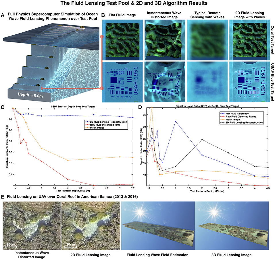
Figure 3. The Fluid Lensing Test Pool, 2D, and 3D Fluid Lensing Algorithm results. (A) A side render of the Fluid Lensing Test Pool showing formation of caustics on floor and optical attenuation (water volume removed for clarity). (B) 2D Fluid Lensing Algorithm Results as compared to a flat fluid state, instantaneous image, and image with integration time. (C,D) Structural Similarity Index (SSIM) and signal-to-noise ratio (SNR) for fluid lensing results as a function of depth. (E) 2D and 3D Fluid Lensing Algorithm results from 2013 and 2016 airborne campaigns in American Samoa. Adapted with permission from Chirayath (2016).
Figure 2 illustrates the basic geometric optics responsible for fluid lensing and the surprising effects they can have on imagery from state-of-the-art commercial marine remote sensing systems. Considering the simplest case of rays propagating from a benthic object through the air-seawater boundary, as depicted in Figure 2A, refraction causes the apparent depth of a benthic object to appear shallower than its true depth, as observed from above the surface. Here, an object O, located at depth d, with respect to mean sea level (MSL), appears as O′ at apparent depth q. Using Snell's law, it can be shown that the actual depth and the apparent depth are related by the refractive depth distortion equation: . With nair = 1 and nseawater = 1.33, this yields q = −0.752d. So, for a flat fluid sea surface and nadir camera viewpoint, the apparent depth is typically three-fourths the actual depth on Earth. This effect appears to magnify an object by an inversely proportional amount. Next, consider the presence of an ocean wave that assumes the form of a small optical lens, or lenslet, of curvature Rlens. For an object O at height p from the lenslet surface, the combined effect of refraction and the curvature of the two-fluid interface will cause light rays emerging from the object to converge at the focal distance q and form image I, as depicted in Figure 2B. Using the small angle approximation for incident light rays, Snell's law becomes nairθ1 = nseawaterθ2. Using exterior angle relations, it can be shown that θ1 = α + β and θ2 = β − γ. Combining these expressions yields nairα + nseawaterγ = β(nseawater − nair). It can be shown that tan(α) ≈ α ≈ d/p, tan(β) ≈ β ≈ d/R, and tan(γ) ≈ γ ≈ d/q. Substituting these linearized expressions into nairα + nseawaterγ = β(nseawater − nair) yields the refractive lenslet image equation:. In the case of the flat fluid surface, R → ∞, and the refractive lenslet image equation yields the refractive depth distortion equation shown earlier: . Finally, in the case of the Sun illuminating a refractive lenslet surface, the refractive lenslet image equation explains the formation of caustic and the phenomenon of caustic focusing from the light gathering area of the lenslet. Figure 2C illustrates the formation of an image, I, at focal point q. Given the angular size of the Sun as viewed from Earth and orbital distance, incident light waves are approximated as planar. With p ≫ R, the refractive lenslet image equation reduced to the following caustic refractive lenslet focusing relation: .
The Fluid Lensing Test Pool
To better understand the effects of ocean wave fluid lensing and create a validation testbed, a full-physics optofluidic simulation was performed on the NASA Ames Pleaides Supercomputer, the fluid lensing test pool (Figure 3A). The 3D full-physics simulation is the first of its kind and includes full water column and atmospheric column absorption, dispersion, scattering, refraction, and multiple reflections, comprising more than 50 million CPU hours for 33 s of animation (Chirayath, 2016). The fluid lensing test pool consists of a series of test targets at various depths submerged in a water volume, with optical properties and surface waves characteristic of the primary target ecosystem, shallow marine reefs in clear tropical waters.
The time-dependent air-water surface is modeled using Tessendorf's Fourier domain method (Tessendorf, 2001) based on a Phillips spectrum of ocean waves from measured spectral features characteristic of a fringing coral reef system. A surface mesh generated from a parameterized Phillips spectrum defines the ocean surface height field h(x, t), represented as the sum of periodic functions such that:
where k is the wave number, k is the wave vector, T is the wave period, λ is the wavelength, h is the height of the water, x is the spatial position of the simulation point, t is time, g is the gravitational constant, Pk is the Phillips spectrum, ξ is an independent draw from a Gaussian random number generator with μ = 0 and σ = 1, L is the largest permissible wave arising from a given wind speed, ω is the angular frequency, and w is the wind direction.
The set of complex Fourier amplitudes and initial phase values at t = 0, is defined by the following expression:
where initial parameters are taken from a Gaussian random number generator, ξi, and Ph(k) is the Phillips spectrum (Phillips, 1958) from wind-driven waves in shallow reef environments. The Phillips spectrum characterizes the spectral and statistical properties of the equilibrium range of wind-generated gravity waves and is generated by the following expression, put forth by Phillips (Phillips, 1985).
The second component of modeling the ocean wave fluid lensing phenomenon is simulating the optofluidic interactions of light with the ocean wave synthesis. Ray-tracing and light transport is used to model optofluidic interactions and is performed using LuxRender v.1.6, a physically-based, open-source, and unbiased render engine. For the purposes of simulating the complex optofluidic interactions specific to the ocean wave fluid lensing phenomenon, this work configures LuxRender to use an efficient CPU-based unbiased bidirectional path tracing render engine with Metropolis Light Transport (MLT) for efficient sampling and caustic convergence.
The ocean wave synthesis is coupled to water's empirically-determined optical properties. The absorptive and refractive properties of seawater are based on experimental data from Pope and Fry (1997) and Daimon and Masumura (2007). From Pope and Fry (1997), it is shown that clear seawater and pure water have similar optical properties relevant to this study; however, the inherent optical properties of real-world marine environments may differ significantly due to suspended sediment, carbon-dissolved organic matter (CDOM), phytoplankton, molecular scattering, and salinity, among other things. The fluid lensing test pool does not model the ocean wave fluid lensing as a function of all of these parameters, but focuses on the dispersive, absorptive, reflective, and refractive properties of water discussed earlier that effectively dominate the fluid lensing phenomenon. However, the framework developed here can easily be extended to model additional complexity in the water column which will be presented in subsequent work.
Based on this modeling work, a number of crucial relationships between surface waves and caustic focusing was discovered and a novel high-resolution aquatic remote sensing technique for imaging through ocean waves, called the general fluid lensing algorithm, was developed (Figure 3) (Chirayath, 2016; Chirayath and Earle, 2016).
The Fluid Lensing Algorithm
The fluid lensing algorithm itself enables robust imaging of underwater objects through refractive distortions from surface waves by exploiting surface waves as magnifying optical lensing elements, or fluid lensing lenslets, to enhance the effective spatial resolution and signal-to-noise properties of remotely sensed images. Primarily a computer vision technique, which utilizes high-frame-rate multispectral video, the fluid lensing algorithm consists of a fluid distortion characterization methodology, caustic bathymetry concepts, fluid lensing lenslet homography technique based on Scale Invariant Feature Transforms (SIFT) and SIFT Flow (Liu et al., 2011), and a 3D remote sensing fluid lensing algorithm as approaches for characterizing the aquatic surface wave field, modeling bathymetry using caustic phenomena, and robust high-resolution aquatic remote sensing (Chirayath, 2016). The formation of caustics by refractive lenslets is an important concept in the fluid lensing algorithm. Given a lenslet of constant curvature, R, the focal point of caustic rays is constant across spatially distributed lenslets. This behavior is exploited for independently determining bathymetry across the test pool in the caustic bathymetry fluid lensing algorithm. It should be noted that the algorithm specifically exploits positive optical lensing events for improving an imaging sensor's minimum spatial sampling as well as exploiting caustics for increased SNR in deep aquatic systems. An overview of the 2D fluid lensing algorithm is presented in Figure 4. The algorithm is presently provisionally-patented by NASA (Chirayath, 2018b).
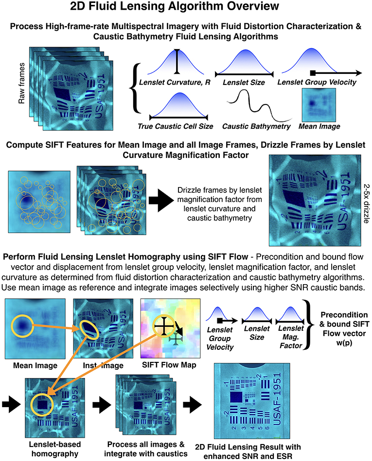
Figure 4. An overview of the 2D Fluid Lensing Algorithm. Adapted with permission from Chirayath (2016).
To validate the general fluid lensing algorithm, the fluid lensing test pool was used to quantitatively evaluate the algorithm's ability to robustly image underwater objects in a controlled environment (Figure 3B) (Chirayath, 2016). Results from the test pool, processed with the 2D fluid lensing algorithm show removal of ocean-wave related refractive distortion of a coral test target and USAF test target, as viewed from a nadir observing remote sensing camera. The “flat fluid image” shows the targets under flat fluid conditions. The “instantaneous wave distorted image” shows targets under typical ocean wave distortions characteristic of shallow marine system sea states. The “typical remote sensing with waves image” shows the 1s integration image, characteristic of present remote sensing sensor dwell times. Finally, the “2D fluid lensing image” with 90 frames (1 s of data) successfully recovers test targets and demonstrates effective resolution enhancement and enhanced SNR from tracking and exploiting fluid lenslets and caustics, respectively.
Results from the fluid lensing test pool were also used to quantitatively validate the fluid lensing algorithm through image quality assessment of reconstructed two-dimensional objects using the Structural Similarity Index (SSIM) (Figure 3C) (Wang et al., 2004) and Signal-to-Noise Ratio (SNR) (Figure 3D). Results from the validation demonstrate multispectral imaging of test targets in depths up to 4.5 m with an effective spatial resolution (ESR) of at least 0.25 cm vs. a raw fluid-distorted frame with an ESR <25 cm, for the case of an airborne platform at 50 m altitude. Note that this result was achieved with an instrument ground sample distance (GSD) of 1 cm, demonstrating a 4-fold increase in ESR from exploitation of positive lensing events. Enhanced SNR gains of over 10 dB are also measured in comparison to a perfectly flat fluid surface scenario with <1 s of simulated remotely-sensed image data, demonstrating fluid lensing's ability to exploit caustic brightening to enhance SNR of underwater targets.
Finally, the algorithm was tested in multiple real-world environments for validation, as discussed in the next section. The ocean wave fluid lensing phenomenon is observed from 2013 and 2016 airborne campaigns in American Samoa. Figure 3E shows an instantaneous (0.03 s integration time) airborne image and 2D fluid lensing image of coral (1 s total integration time). Note the branching coral is completely unresolvable in the instantaneous image, while caustics introduce significant noise, especially over the sandy pavement region. The fluid lensing image resolves the coral and sandy benthic floor accurately. These refraction corrected results are used alongside a fluid lensing caustic bathymetry algorithm and structure from motion algorithms to create a 3D fluid lensing image and the wavefield can be inversely estimated to render the distortions again (Figure 3E).
FluidCam Instrument and Airborne Field Campaigns
The fluid lensing algorithm eventually necessitated the development of dedicated high-frame-rate multispectral full-frame focal plane arrays (FPAs) and powerful heterogeneous computing architectures, which motivated the development of dedicated instruments, NASA FluidCam 1&2 (Chirayath and Instrella, 2016), shown in Figure 5, and follow-on hardware and software optimizations through SpaceCubeX (Schmidt et al., 2017), for scaling to CubeSat form factors and power constraints.
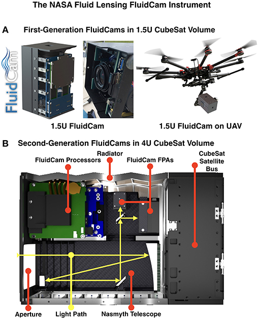
Figure 5. The NASA Fluid Lensing FluidCam instrument. (A) A cutaway render and image of the first-generation FluidCam, which fits in a 1.5 U CubeSat volume is shown alongside the instrument mounted on a UAV for airborne mapping missions. (B) The second-generation FluidCam consists of a 4 U instrument payload for a 6 U CubeSat. The new architecture affords multiple larger focal plane arrays, improved optical performance, and a heterogeneous CPU/GPU processing stack optimized through the SpaceCubeX project.
FluidCam 1 & 2, custom-designed integrated optical systems, imagers and heterogeneous computing platforms were developed for airborne science and packaged into a 1.5 U (10 × 10 × 15 cm) CubeSat form factor (Figure 5A) with space capable components and design. Since 2014, both FluidCam 1 (380–720 nm color) and FluidCam 2 (300–1,100 nm panchromatic) have been actively used for airborne science missions over a diverse range of shallow aquatic ecosystems and contributed data for research in the broader international biological and physical oceanographic community (Suosaari et al., 2016; Purkis, 2018; Rogers et al., 2018; Chirayath and Instrella, accepted; Chirayath and Li, in review). The 3D Fluid Lensing Algorithm was validated on FluidCam from aircraft at multiple altitudes in real-world aquatic systems at depths up to 10 m (Figures 3E, 6). Field campaigns were conducted over coral reefs in American Samoa (2013, 2016) (Chirayath and Earle, 2016; Rogers et al., 2018), stromatolite reefs in Western Australia (2014) (Suosaari et al., 2016), and freshwater riverine systems in Colorado in 2018, with 10 more field campaigns planned 2019–2020 for the NeMO-Net project. Fluid lensing datasets revealed these reefs in high resolution, providing the first validated cm-scale 3D image of a reef acquired from above the ocean surface, without wave distortion, in the span of a few flight hours over areas as large as 15 km2 per mission. The data represent the highest-resolution remotely-sensed 3D multispectral image of a marine environment to date. Figure 7 shows an inset comparing a transect of coral in American Samoa in 2013 and 2016, showing the potential for change detection at fine spatial and temporal scales using this methodology.
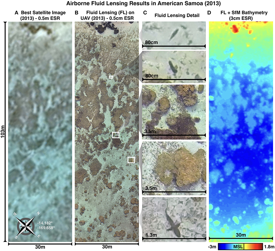
Figure 6. The first airborne fluid lensing results from an experimental 2013 campaign in American Samoa. (A) Highest-resolution publicly available image of a transect area captured June 2015 from Pleiades-1A satellite with 0.5 m ESR. (B) Fluid lensing 2D result of the same area as captured from UAV at 23 m altitude with estimated 0.5–3 cm ESR. (C) Inset details in fluid lensing 2D image include a parrotfish ~20 cm in length, a sea cucumber ~21 cm in length, multiple coral genera including Porites and Acropora, and a reef shark. (D) High-resolution bathymetry model generated with fluid lensing caustic bathymetry (FL) and Structure from Motion (SfM) algorithms, validated by underwater photogrammetry. Maximum depth in model is ~3 m, referenced to mean sea level (MSL). Adapted with permission from Chirayath (2016).
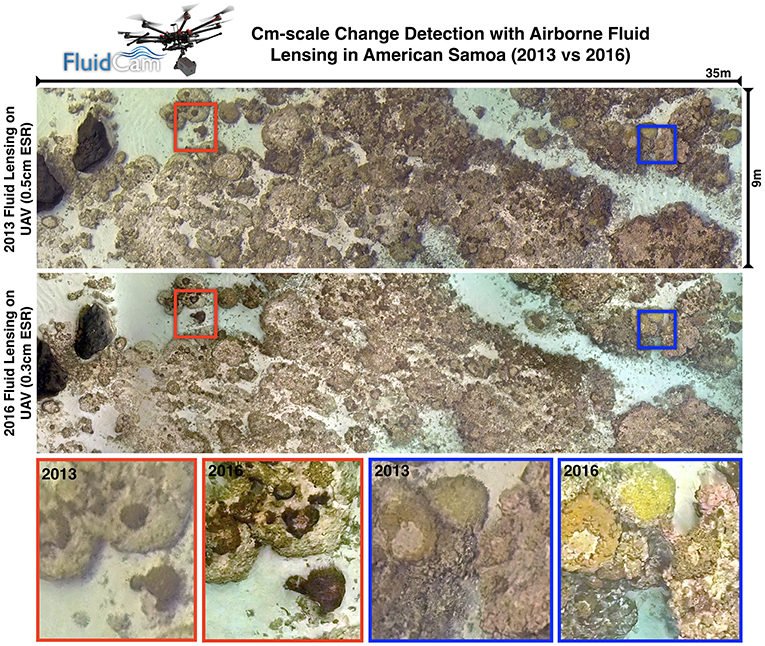
Figure 7. Cm-scale change detection from airborne fluid lensing in American Samoa. Here, 2013 airborne fluid lensing data from a patch of reef are compared with a repeat survey in 2016 showing cm-scale changes in the reef. Color coded regions compare similar areas in each image and show a change in ratio of coral types as well as coral cover. The increased ESR and improved SNR of the 2016 data reflect software and hardware advances in the development of the FluidCam instrument.
While FluidCam 1&2 were designed as instruments for future in-space validation with components selected that met vibrational, thermal and atmospheric requirements, a second-generation system was designed into a 4 U form-factor with improved computational capability, redundant data storage, a custom optical telescope, fully radiative cooling and carbon fiber chassis, and updated high-bandwidth multispectral focal plane arrays. Figure 5B shows the 4 U FluidCam payload. The optical telescope has been redesigned from the first generation and consists of a proprietary square-aperture Nasmyth focus Ritchey-Chretien reflecting telescope based on a design proposed by Jin et al. (2013).
Airborne field campaign results, along with validation results from the Fluid Lensing Test Pool, suggest the 3D Fluid Lensing Algorithm presents a promising advance in aquatic remote sensing technology for large-scale 3D surveys of shallow aquatic habitats, offering robust imaging capable of sustained shallow marine imaging. However, while the highlights presented here demonstrate applicability of the Fluid Lensing Algorithm to the tested environments, further investigation is needed to fully understand the algorithm's operational regimes and reconstruction accuracy as a function of the inherent optical properties of the water column, turbidity, surface wave fields, ambient irradiance conditions, and benthic topography, among other considerations. Current and future work is already underway to study the impact of these variables on the fluid lensing algorithm and its application to aquatic remote sensing as a whole. This research is ongoing with algorithm performance improvements, FluidCam imaging and processing hardware maturation, and automated fluid lensing dataset analysis tools such as NeMO-Net.
MiDAR—The Multispectral Imaging, Detection, and Active Reflectance Instrument
While FluidCam and fluid lensing offer a new technique for improved passive remote sensing of aquatic systems, they are passive sensing methods, reliant on the Sun's downwelling irradiance, and thus limited to the photic zone of the ocean. This inspired the development of an active multispectral sensing technology that could extend the penetration depth of remote sensing systems. Here, we share preliminary results and developments behind the recently-patented NASA Multispectral Imaging, Detection, and Active Reflectance Instrument (MiDAR) and its applications to aquatic optical sensing and communications (Chirayath, 2018a).
Active remote sensing technologies such as radio detection and ranging (RADAR) and light detection and ranging (LiDAR) are largely independent of ambient illumination conditions, provided sufficient transmitter irradiance over background, and advantageously contend with attenuation along the optical path by exploiting phase information using heterodyne receivers. Thus, hardware requirements for receiver sensitivity, aperture and SNR can effectively be relaxed given increased transmitter power (up to MW of power in the case of RADAR). Recent advances in LiDAR have also enabled multiple wavelengths of laser diodes to be used simultaneously in green and two infrared bands to achieve a “color” LiDAR point cloud (Briese et al., 2012, 2013). However, multispectral LiDAR methods are not yet applicable to imaging across the visible optical regime as there exist significant limitations in narrowband laser-diode emitter chemistry and efficiency.
Recent advances in active multispectral imaging have explored the concept of multiplexed illumination via light-emitting diode (LED) arrays to dynamically illuminate a scene, reconstructing the spectral reflectance of each pixel through model-based spectral reconstruction through a charge-coupled device (CCD) detector (Nischan et al., 2003). Most prototypes at this stage have been relatively low power (~10 W), stationary, and unable to achieve the levels of irradiance required for remote sensing applications at larger distances, and hence have been predominantly been purposed for the task of object detection, relighting and close-up monitoring (Park et al., 2007; Parmar et al., 2012; Shrestha and Hardeberg, 2013). However, results have shown significant promise in the system's ability to reveal key features in the spectral domain, reconstruct spectra with surprising accuracy (Goel et al., 2015), and operate in conditions where an active illumination source can be directly controlled as required. In the field of multispectral video, passive systems employing dispersive optical elements through scene-scanning or bandpass filtering (Yamaguchi et al., 2006), while providing high spectral resolution, are unsuitable for achieving high framerates due to limited ambient illumination.
Motivated by the challenges discussed above, MiDAR was developed in pursuit of a next-generation sensing technology capable of expanding the use of multispectral/hyperspectral optical sensing to the seafloor. For aquatic optical sensing, the goal of MiDAR is to reach a state of parity with terrestrial remote sensing. Namely, to develop an instrument capable of reaching beyond the photic zone with active sensing and integration on AUVs for seafloor mapping.
MiDAR Overview
MiDAR is an active multispectral/hyperspectral system capable of imaging targets with high-intensity narrowband structured optical radiation to measure an object's spectral reflectance, image through fluid interfaces, such as ocean waves, with fluid lensing, and simultaneously transmit high-bandwidth data. MiDAR consists of an active optical transmitter (MiDAR transmitter) and passive receiver (MiDAR receiver) in either a monostatic or bistatic configuration (Figures 8A,C). The MiDAR transmitter emits coded narrowband structured illumination to generate high-frame-rate multispectral video, perform real-time spectral calibration per color band, and provide a high-bandwidth simplex optical data-link under a range of ambient irradiance conditions, including darkness. A schema of a bistatic MiDAR, typically used for aquatic remote sensing, is shown in Figure 8C as a payload aboard a UAV. The MiDAR receiver, a high-framerate panchromatic focal plane array coupled to a heterogeneous computing stack, passively decodes embedded high-bandwidth simplex communications while reconstructing calibrated multispectral images. A central goal of MiDAR is to decouple the transmitter from the receiver to enable passive multispectral synthesis, robustness to ambient illumination, optical communications, and the ability to select particular multispectral color bands on the fly as a function of changing mission requirements. The MiDAR transmitter and receiver utilize cost-effective components and relax sensitivity requirements on the receiving aperture to achieve multispectral video at a SNR that can be directly modulated from the MiDAR transmitter.
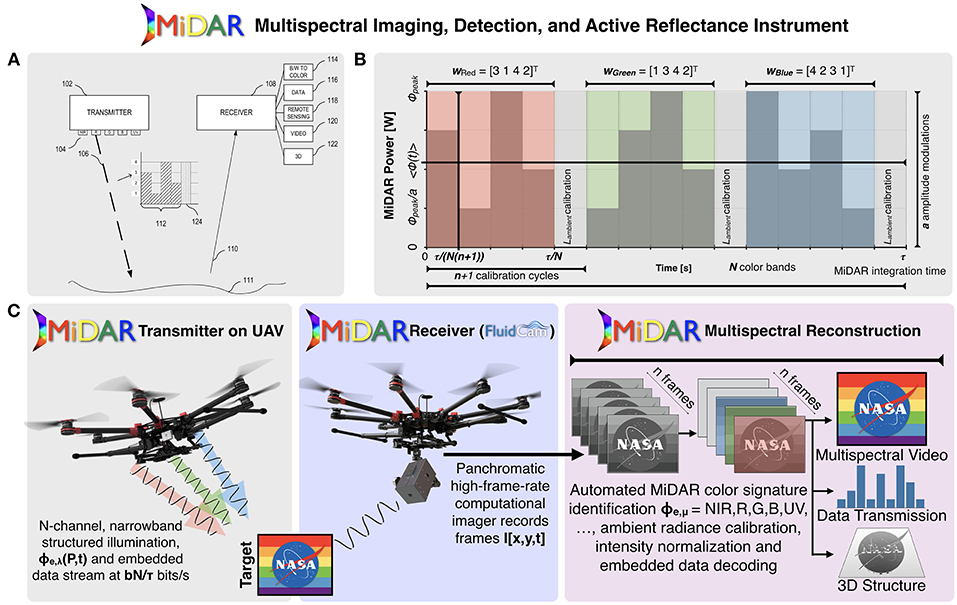
Figure 8. MiDAR, the NASA Multispectral, Imaging, Detection, and Active Reflectance Instrument. (A) MiDAR is an active multispectral/hyperspectral instrument that uses multiple narrowband optical emitters to illuminate a target with structured light (MiDAR Transmitter). The reflected light is captured by a telescope and high-frame-rate panchromatic focal plane array (MiDAR Receiver) with a high-performance onboard heterogenous computing stack, which creates hyperspectral images at video framerates, and decodes embedded optical communications in real-time (Chirayath, 2018a). (B) The structured illumination pattern generated by the MiDAR transmitter allows for simultaneous optical communication and calibrated measurement of a target's reflectance at multiple wavelengths, independent of ambient illumination conditions. (C) MiDAR can be operated in a bistatic or monostatic configuration. For remote sensing applications, MiDAR has been tested on UAVs.
MiDAR multispectral image synthesis is premised upon the following physical approximations:
1. Light is reflected instantaneously from target surfaces. Phosphorescent materials thus are characterized by only by their reflectance.
2. Incoming light from the MiDAR transmitter is reflected from the target surface at the same wavelength. Fluorescent emission can be characterized using a special MiDAR receiver.
3. There are limited participating media. Primary reflectance occurs at a surface element rather than scattering within a material.
4. The bidirectional reflectance distribution function (BRDF) is a function only of three variables, f(θi, θr, ϕi − ϕr), where θi, θr, ϕi, ϕr are the respective incident and reflected zenith and azimuthal angles and reflectance is rotationally invariant about the target surface normal.
5. Helmholtz reciprocity applies such that BRDF satisfies f(θi, ϕi; θr, ϕr) = f(θr, ϕr; θi, ϕi).
6. MiDAR transmitter power, ϕe, peak, at range R, results in signal irradiance that is much greater than ambient irradiance, Iambient. (IMiDAR ≫ Iambient).
7. Target reflectance and scene do not change on timescales faster than the MiDAR receiver frequency, fRx (90 Hz−36,000 Hz for NASA FluidCams).
8. MiDAR receiver frequency fRx is at least two times greater than MiDAR transmitter driving frequency fTx. (fRx > 2fTx).
The MiDAR Transmitter
The MiDAR transmitter achieves narrowband optical illumination of a target at range R with an array of efficient high-intensity laser or light emitting diodes (LEDs) grouped into N multispectral color bands, μ. MiDAR transmitter spectral bands, and their associated emitter diode chemistries, are shown in Figure 9B. The laser and LED array, or MiDAR transmitter, is driven by a periodic variable-amplitude input signal to emit modulated structured light. ϕe, λ (P, t) G(λ) is the time-varying, emitted spectral radiant power distribution of the MiDAR transmitter [Wnm−1s−1], where G(λ) is the gain of the MiDAR transmitter at wavelength λ. Each MiDAR color band, μ, spanning spectral range λ, is assigned a unique amplitude-modulated signature, MiDAR signature wμ, defined by modulating the peak power in a color band, ϕe, peak, according to coefficients in column vector wμ, consisting of n irradiance calibration cycles per color band, a amplitude modulation levels and one ambient irradiance calibration cycle (Figure 8B). For all color bands, these column vectors form a nxN MiDAR coefficient
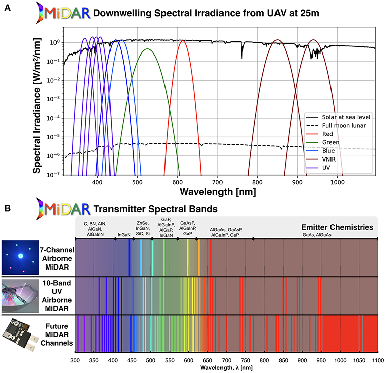
Figure 9. MiDAR power and spectral coverage. (A) MiDAR can operate with zero ambient illumination, but also in the presence of ambient light. A 10-band kw-class airborne MiDAR system is under development that matches or exceeds the solar downwelling irradiance from a UAV at 25 m altitude. Typically, MiDAR is used exclusively at twilight and night for maximum SNR, in which case the SNR typically exceeds that of passive instruments by orders of magnitude. (B) Multiple MiDAR transmitters have been developed or are presently under development that span the UV-NIR optical spectrum. Emitter chemistries have been identified for each spectral channel that allow for high luminous efficiency.
Reflecting optics are used to distribute the radiation pattern Υ(x, y) uniformly across the scene while N total multispectral color bands μ = NIR, R, G, B, UV, … (Figure 9B) are cycled through in total MiDAR integration time seconds (Figure 8B). Modulating power based on coefficients in the weight matrix W allows for passive detection, independent color band recognition and irradiance normalization by a panchromatic MiDAR receiver. This scheme, subject to the constraints Equation 1, below, allows the MiDAR transmitter to alter the color band order and irradiance in real-time, relying on the MiDAR receiver to passively decode the embedded information and autonomously calibrate to changing illumination intensity. Further, MiDAR signatures allow the transmitter and receiver to operate in a monostatic or bistatic regime with no communication link beyond the embedded optical signal. For additional bandwidth, color bands may have b redundant MiDAR signatures, allowing for b bits of data to be encoded at a bitrate of bit/s.
The MiDAR signature for each color band, ϕe, μ, must remain unique to μ across ϕ(t) (Equation 1, ii). For uniform SNR across the color bands, the average integrated power 〈ϕ(t)〉 must be constant over τ/N (Equation 1, i). Finally, to maximize the multispectral video frame-rate, SNR and data transmission bandwidth, the optimization problem in Equation 1 must be solved to minimize τ.
MiDAR transmitter signal optimization problem and constraints for minimum multispectral integration time, maximum bandwidth and uniform SNR.
MiDAR receiver image reconstruction, discussed in the following section, composes the final multispectral image from a weighted average of decoded frames. In the limit of an ideal system, the SNR of a monostatic MiDAR system at a particular wavelength, λ, is proportional to the expression in Equation 2.
Idealized MiDAR SNR proportionality for a color band at wavelength λ where ϕpeak(λ) is the peak power input to the MiDAR transmitter at wavelength λ and G(λ) is the gain of the MiDAR transmitter at wavelength λ. Ar is the MiDAR receiver area, ΩFOV is the field of view, Lambient(λ) is the ambient radiance at wavelength λ and R is the range.
MiDAR Receiver
A passive, high-frame-rate panchromatic FPA coupled to a computational engine functions as the MiDAR receiver. The MiDAR receiver samples reflected structured light from the illuminated object at the MiDAR receiver frequency, fRx. Onboard algorithms digitally process the high-frame-rate image data to decode embedded simplex communication, perform in-phase intensity and color-band calibration and reconstruct a N-band calibrated multispectral scene at a framerate of τ−1 Hz. The MiDAR prototype highlighted here uses the NASA FluidCam instruments as MiDAR receivers.
MiDAR Receiver Multispectral Video Reconstruction Algorithm
The MiDAR receiver digitizes sequential panchromatic images I[x, y, t] at {Nx, Ny} pixels and framerate fRx Hz. N ambient radiance calibration cycles are used to calibrate intensity and the normalized image sequence is then difference transformed:
This method permits varying gains per channel and is robust to noise as a function of the subject being imaged. Note that the length of I here is the same length as w, and mirrors the relative signature pattern of w. The final transformed u is then cross-correlated with the MiDAR coefficient matrix to detect and assign color bands. The MiDAR multispectral reconstruction algorithm composes a calibrated [Nx x Ny] x N x t dimensional multispectral video scene consisting of N color bands, μ. The multispectral video matrix, M[x, y, μ, t], is constructed from a weighted average of color-band classified panchromatic images I[x, y, t] over total integration time τ.
MiDAR Optical Communications Decoding Algorithm
Additional simplex communications may be simultaneously embedded in the MiDAR transmitter's spectral radiant power distribution, ϕe, λ (P, t). By creating b redundant MiDAR color signatures ϕe, μ, simplex data can be transmitted at a minimum rate of bit/s with no loss to MiDAR multispectral image SNR. For a panchromatic FluidCam-based MiDAR receiver, for example, with fRx = 1550Hz, N = 32 color bands, a = n = 5 amplitude modulation and calibration cycles and b = 10 redundant MiDAR signatures, this algorithm can achieve a data-rate of 2.58 kbps while performing imaging operations. Using a passive color sensor as the MiDAR receiver, such as the multispectral FluidCam with K color channels, this bandwidth can be increased by simultaneous transmission of multiple MiDAR color bands. In the case that a MiDAR receiver has K = N matching color bands, the data rate increases to bit/s, or 82.67 kbps.
MiDAR can be used for long-range optical communications using this methodology with the MiDAR receiver pointed directly at the MiDAR transmitter for increased gain. The SNR for b bits of data transmitted at wavelength λ is then proportional to:
Full descriptions of the MiDAR Receiver Multispectral Video Reconstruction Algorithm and Optical Communications Decoding Algorithm are provided in the MiDAR patent (Chirayath, 2018a).
MiDAR Instrument Development and Preliminary 7-Channel Airborne MiDAR Results
MiDAR transmitter and receiver hardware are currently under active development. Five, seven, and thirty-two band MiDAR transmitter prototypes have thus far been developed with total peak luminous power ratings up to 200 watts and spectral ranges from far UV to NIR, suitable for in-situ and short-range active multispectral sensing (Figure 9B). A number of light-emitting diode chemistries have been tested and identified that span much of the UV-NIR electromagnetic spectrum for future implementations (Figure 9). Currently, a 10-band airborne kW-class MiDAR transmitter is in development featuring four UV-band channels. This transmitter is designed to fly on a UAV for active multispectral imaging at an altitude of 25 m. At this altitude, the transmitter is expected to match downwelling solar irradiance at noon, but will operate primarily during twilight and evening for increased SNR (Figure 9A). Compared to daytime passive remote sensing observations with full downwelling solar irradiance, nighttime MiDAR observations with a full lunar phase downwelling irradiance will have a SNR 10-103 times higher in the case of a UAV at 25 m altitude.
Figure 10A shows results from a basic laboratory test of a 7-channel airborne MiDAR in Figure 9B. Here, a monostatic MiDAR system is tested using the 7-channel transmitter mounted on an optical bench, collocated with FluidCam as a receiver. The monostatic system was targeted at a multispectral test target 2 m away under constant diffuse, broad-spectrum ambient lighting conditions of ~1 W/m2. MiDAR parameters for this experiment were: N = 7, fTx = 100Hz, n = a = 4, {Nx, Ny} = {1024, 1024}, fRx = 365Hz, τ = 0.25s.
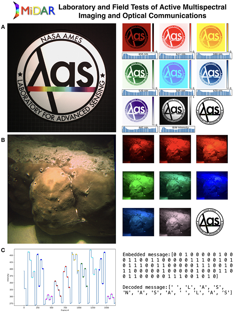
Figure 10. MiDAR Laboratory and Field Tests of Active Multispectral Imaging and Optical Communications. (A) 7-Channel monostatic MiDAR imaging test on optical bench with multispectral test target. Here, half of the test target was illuminated with a broadband source to test MiDAR's ability to determine active reflectance independent of ambient conditions. RGB image shown on left. Reflectance maps shown for each spectral band from 655 to 447 nm on right. (B) The first 7-channel airborne MiDAR test over coral with an underwater MiDAR receiver from a 2018 field campaign in Guam. Here, MiDAR is operating in a bistatic configuration with a MiDAR transmitter above the surface, and a diver-mounted MiDAR receiver underwater. MiDAR resolves a Porites coral in the same seven multispectral bands as the optical bench test, and simultaneously performs simplex optical communication through the air-water interface. (C) Embedded MiDAR data transmission in coral image decodes a simple hidden message.
Figure 10B presents results from a 2018 bistatic MiDAR field test in Guam with the 7-channel airborne transmitter above the air-water interface at 1 m illuminating a Porites coral at a depth of 1 m. The MiDAR receiver is located under the water at a range of 1 m from the coral head. Here, similar MiDAR parameters were used as for the laboratory test. In addition, a simplex transmission was encoded during imaging through the air-water interface. The decoded signal and message are shown in Figure 10C.
The MiDAR transmitter spectral radiant power distribution, ϕe, λ (P, t) was produced using a 7-channel array of narrowband LEDs (Figure 9B), centered at 447, 470, 505, 530, 590, 627, and 655 nm wavelengths with full-width-half-maximum (FWHM) values of Δλ = 10, 25, 35, 15, 35, 35, and 37 nm, respectively. The LED array was driven by microsecond, pulse-width-modulated (PWM) signals generated by an Arduino Uno microprocessor with high-current switching performed by MOSFETs. LED power per color was chosen to compensate for transmitter gain losses, G(λ) and receiver losses such for an average emitted power 〈ϕe, λ (P, t) G(λ) 〉 = 10Watts.
Potential Applications of MiDAR to the Earth and Space Sciences
Preliminary MiDAR results at low transmission power (~10 W) offer promising developments in active optical sensing that are applicable to aquatic systems. As higher-power kW-class MiDAR transmitters are matured, there are a number of potential applications of this technology to Earth and Space Sciences including high-resolution nocturnal and diurnal multispectral imaging from air, space and underwater environments as well as optical communication, bidirectional reflectance distribution function characterization, mineral identification, UV-band imaging, 3D reconstruction using structure from motion, and active fluid lensing for imaging deeper in the water column (Figure 11). Multipurpose sensors such as MiDAR, which fuse active sensing and communications capabilities, may be particularly well-suited for mass-limited robotic exploration of Earth and other bodies in the solar system.
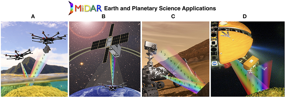
Figure 11. MiDAR Earth & Planetary Science Applications. (A) Airborne MiDAR depicted operating over coral system with FluidCam in bistatic configuration. (B) MiDAR operating as high-bandwidth communications link to satellite system from same airborne transmitter. (C) MiDAR system integrated onto Mars rover for hyperspectral and UV sensing of facies. (D) MiDAR system integrated onto deep sea AUV for active multispectral benthic remote sensing in light-limited environment. Background image credit: NASA.
NeMO-Net—Neural Multi-Modal Observation and Training Network for Global Coral Reef Assessment
Driven by the need for multimodal optical sensing processing tools for aquatic systems, as well as a toolkit to analyze and exploit the large (TB and PB scale) datasets collected from FluidCam and MiDAR, the NeMO-Net project was initiated in late 2017 (Chirayath et al., 2018a,b). NeMO-Net is highlighted here as an example of a scalable data fusion and processing information systems development that aims to make use of optical datasets from a variety of instruments to answer questions of global scale for aquatic ecosystems. Specifically, NeMO-Net is an open-source deep convolutional neural network (CNN) and interactive active learning training software designed to accurately assess the present and past dynamics of coral reef ecosystems through determination of percent living cover and morphology as well as mapping of spatial distribution (Cartier, 2018). NeMO-Net exploits active learning and data fusion of mm-scale remotely sensed 3D images of coral reefs from FluidCam and MiDAR as well as lower-resolution airborne remote sensing data from commercial satellites providers such as Digital Globe and Planet, as well as NASA's Earth Observing System data from Landsat, to determine coral reef ecosystem makeup globally at the finest spatial and temporal scales afforded by available data.
Previously, it was shown that mm-scale 3D FluidCam imagery of coral reefs could be used to improve classification accuracies of imagery taken from lower-resolution sensors through a communal mapping process based upon principal component analysis (PCA) and support vector machines (SVM) (Chirayath and Li, in review). This work further showed that supervised learning of FluidCam data can be used to identify spectral identification data from higher-dimensional hyperspectral datasets for coral reef segmentation. Consequently, the scope of this work was expanded with the development of NeMO-Net, utilizing supervised and semi-supervised CNNs to recognize and fuse definitive spatial-spectral features across coral reef datasets.
NeMO-Net CNN Architecture
On a high level, CNNs are modeled upon the human image recognition process, where sections of the field of view are independently synthesized and collated over multiple layers (i.e., neurons) to form abstract and high level feature maps which are generally robust and invariant (Lecun et al., 1998). This can be extended to the remote sensing case, where a combination of spatial-spectral properties may be more reflective of segmentation criteria than a single-faceted approach. However, CNNs have only very recently been examined as an alternative to conventional methods for image classification and thematic mapping, and as such is currently an area of active research with many unexplored possibilities (Gomez-Chova et al., 2015).
The structure of NeMO-Net's CNN is shown in Figure 12. The input to the CNN is an image or a set of images (different spectral bands and spatial resolutions in our case). The convolution step is used to extract a set of filters through back-propagation, by applying 3 × 3 convolutions, for example, that are smaller in size than the original image. During the next step, pooling is used to reduce the spatial scale of the filtered images, often down-sampling by a factor of two per dimension. This process can be repeated several times, depending on the image size and feature complexity. Finally, the results from pooling are fed into a fully connected layer where probabilistic votes are combined to predict the class based upon previously trained ground-truth samples. A distinct advantage of the CNN scheme over the standard multi-layer perceptron (MLP) NN schemes is their ability to ingest 2D (e.g., images) or 3D (e.g., spectral images), or higher-dimensional datasets, as direct inputs, whereas the inputs for MLP-NN depend heavily on pre-processing and dimensionality reduction in order for the network to achieve good prediction, and sometimes even to reach convergence. Another advantage of the pooling process inherent with CNN is its low sensitivity to the exact position or skewness of the feature (up to a certain extent), allowing for the augmentation of noisy images. At present, CNNs have already shown promise in remote sensing areas such as land use, hyperspectral, and satellite image classification (Castelluccio et al., 2015; Chen et al., 2016; Zhong et al., 2017) with greatly increased classification accuracies. Challenges remain, however, especially since tuning large CNNs often require an abundance of training data and significant computational power. To this end, NeMO-Net incorporates a citizen-science based active learning and training application as well as utilizing the NASA Ames Pleaides Supercomputer and NASA Earth Exchange (Figure 13).
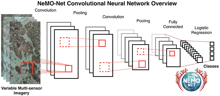
Figure 12. NeMO-Net Convolutional Neural Network (CNN) Overview. NeMO-Net's CNN is designed to perform multiresolution, multispectral, multitemporal, multisensor feature extraction, and classification for optical remote sensing data. Independent data sources are fed into the CNN, in which convolution, pooling, and fully connected layers are implemented to extract invariant features. Final predictions are made according to logistic regression upon relevant classes.
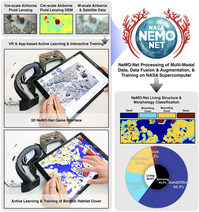
Figure 13. NeMO-Net is aimed at harmonizing the growing diversity of remote sensing and in situ imagery into a single open-source platform for assessing shallow marine ecosystems at scale across the globe. An active learning game, playable on tablet and virtual reality platforms, allows users to view 3D FluidCam data of coral reefs and provide training data on coral classes including living cover, morphology type, and family identification. These data, along with their spatial coordinates, are fed into NeMO-Net, which produces a classification map and reef constituent breakdown as well as error analysis based upon training data. This technology is presently under development and will be expanded to third-party georeferenced 3D datasets as well.
As primarily an information systems development project, NeMO-Net's overall technical goals are to: (1) develop a malleable CNN architecture specific to aquatic optical sensing datasets for scalable heterogenous computing architectures such as the NASA Ames Pleaides Supercomputer, (2) create a cloud and cloud shadow detection CNN algorithm for masking (Segal-Rozenhaimer et al., accepted), (3) implement domain transfer learning for spectral and spatial resolution transfer learning (super resolution) across multiple sensors, and (4) create a 3D active learning CNN training application in game interface for data training from multiple sensors. NeMO-Net's science objectives include: (1) Developing an accurate algorithm for identification of coral organisms from optical remote sensing at different scales. (2) Globally assessing the present and past dynamics of coral reef systems through a large-scale active learning neural network. (3) Quantifying coral reef percent cover and spatial distribution at finest possible spatial scale. (4) Characterizing benthic habitats into 24 global geomorphological and biological hierarchical classes, resolving coral families with fluid lensing at the finest scales and geomorphologic class at the coarsest scale.
Often the most challenging and limiting aspects of CNNs, such as NeMO-Net, are CNN learning and label training; that is associating pixels in remote sensing imagery with mapping labels such as coral or seagrass. On this topic, the three prevalent issues are:
1) The labeled data is not representative of the entire population distribution. In coral reefs, for example, labels often only correspond to reefs within their immediate geographical vicinity, which are known to vary compositionally and structurally worldwide. This can lead to significant generalization error when learned CNN models are tested on particular samples and evaluated upon data points from other areas.
2) The number of available labels is very small (~1% of the data), where the most common criticism associated with CNNs is their dependence upon a vast amount of labeled training data.
3) Spectral mixing and 3D structure confusion occurs in areas of high benthic heterogeneity, conflating multiple ecological classes into small areas.
To address the first and third issues, NeMO-Net utilizes a technique called transfer learning. To address the data skewness issue, for example, NeMO-Net can utilize areas where extensive training label data exist concurrent with instrument data (Chirayath and Earle, 2016; Chirayath and Instrella, 2016). Feature representation learned by the CNN on this dataset is then used to augment the feature representation of other regions. Deep features extracted from CNNs trained on large annotated datasets of images have been used as generic features very effectively for a wide range of vision tasks, even in cases of high heterogeneity (Donahue et al., 2014). To address the second issue, NeMO-Net utilizes virtual augmentation of data. Here, existing labeled data are subjected to a series of transformations such as spatial rotation, decimation, radiation-specific and mixture-based techniques to reinforce robustness of the algorithm. This allows the simulation of radiometric attenuation, spectral mixing, and noise effects inherent to any spectral based sensing platform.
Additional components of NeMO-Net include the use of semi-supervised learning. Semi-supervised classification combines the hidden structural information in unlabeled examples with the explicit classification information of labeled examples to improve classification performance. The objective here is such that given a small sample of labeled data and a large sample of unlabeled data, the algorithm will attempt to classify the unlabeled data through a set of possible assumptions, such as smoothness/continuity, clustering, or manifold representation. Supervised learning in the context of CNNs can be accomplished through pseudo-labels by maximizing the class probabilities of the unlabeled data pool (Lee, 2013). Other approaches include use of standard supervised learning methods such as non-linear embedding (MDS, Isomap) in combination with an optimization routine at each layer of the deep network for structure learning on the unlabeled pool (Weston et al., 2012).
Finally, NeMO-Net augments labeled data through active learning. Active learning is an area of machine learning research that uses an “expert in the loop” to learn iteratively from large data sets that have very few annotations or labels available. In the case of NeMO-Net, the users classifying objects are humans in the loop and the active learning strategy algorithm decides which sample from the unlabeled pool should be given to the expert for labeling such that the new information obtained is most useful in improving the classifier performance. Common strategies include most likely positive (Sharma et al., 2016) and uncertainty sampling (Lewis and Catlett, 1994). The interactive NeMO-Net tablet application is used for active learning (Figure 13).
The overall algorithmic architecture for NeMO-Net is shown in Figure 14 and consists of:
1) Preprocessing of multiplatform data: this includes image registration, scaling and noise removal from affected datasets, allowing easy ingestion into the CNN regardless of sensor platform.
2) NeMO-Net training is performed by providing a multitude of classification images from various sources, covering a wide spatial, spectral, and temporal range. The goal is such that the CNN is able to extract high level spatial-spectral features that are inherent across all relevant datasets. As mentioned previously, to alleviate the issue of labeled data shortage, techniques such as virtual data augmentation, semi-supervised learning, and active learning methods are be used.
3) To address the issue of data overfitting, regularization, dropout, and activation function selection are used (Krizhevsky et al., 2012).
4) Parameter tuning is performed via a validation set and error analysis performed through cross-analysis against a reference set, designed to gauge the robustness, predictive capability and error characteristics of the system.
5) Final classifications are calculated via logistic regression into relevant classes. In cases where multiple temporal and spatially co-registered datasets are available, fusion of multiple CNN outputs by ensemble or Bayesian inference techniques is implemented.
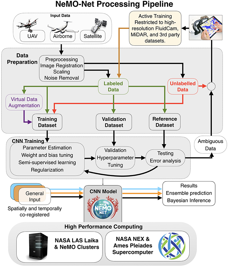
Figure 14. NeMO-Net Processing Pipeline. UAV, airborne, and satellite data are preprocessed and split into labeled and unlabeled categories. Relevant training, validation, and reference sets are created and fed into the CNN training process. Ambiguous data sets are fed back into an active training section for active learning. The final CNN model takes spatially and temporally co-registered datasets, if available, and outputs predictions based upon ensemble or Bayesian inference techniques.
NeMO-Net Preliminary Results
Presently, NeMO-Net's CNN is implemented through an open-source Python package that can be integrated with QGIS, an open source geographical information system. With this pairing, the CNN learning module has access to other useful services such as geolocation, layered data, and other classification tools for comparison. The Python package is also designed to build upon and integrate with existing libraries for machine learning and modern geospatial workflow, such as TensorFlow, Scikit-learn, Rasterio, and Geopandas. To increase computational speed, NeMO-Net takes advantage of heterogenous CPU and GPU processing on the NASA High-End Computing Capability (HECC) Pleiades supercomputing cluster, located at NASA Ames. The active learning application has been developed on the game development platform Unity Pro and 3D modeling software Maya LT for iOS, with a server for data storage and transfer.
Figure 15 shows an example of NeMO-Net's prototype cm-scale benthic map product from FluidCam, based on field data from American Samoa shown earlier. The reef transect was classified into four classes; sand, rock, mounding coral, and branching coral. Using 0.2% of randomly-sampled label data for training the NeMO-Net CNN is able to predict the entire benthic map from FluidCam data with a total accuracy across all four classes of 94.4%. This result is compared to the 92% accuracy (8% error) achieved at the cm spatial scale in Figure 1 using an independent methodology based on MAP estimation (Chirayath and Instrella, accepted).
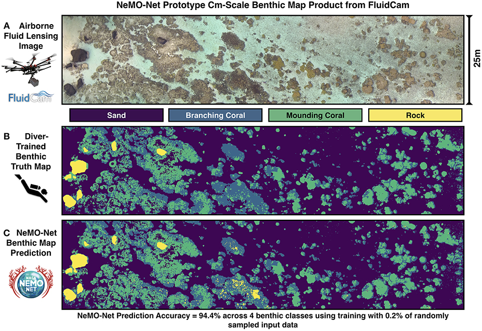
Figure 15. Preliminary NeMO-Net CNN benthic mapping predictions using FluidCam data. (A) Cm-scale 2D and 3D multispectral data are input into NeMO-Net from airborne fluid lensing campaigns. (B) To test accuracy of NeMO-Net prediction, divers meticulously surveyed this entire transect to produce a benthic habitat map of the coral reef to use as truth, or reference data (Chirayath and Instrella, accepted). The reef transect was classified into four classes; sand, rock, mounding coral, and branching coral. (C) The diver data were randomly sampled to label 0.2% of the FluidCam data for training the NeMO-Net model on the NASA Ames Supercomputer. As a result, the NeMO-Net CNN is able to predict the entire benthic map from FluidCam data (A), with a total accuracy across all four classes of 94.4%.
Discussion and Future Work
The three emerging NASA technologies shared here begin to address some of the ongoing observational, technological, and economic challenges encountered in marine sensing, particularly as they apply to coral reef ecosystems.
FluidCam has been utilized extensively on UAVs for scientific surveys of shallow marine environments in small areas, ~15 km2 at a time. The fluid lensing algorithm has provided a robust way to survey shallow marine ecosystems under various sea states at high-resolution in 3D. In addition, FluidCam and fluid lensing have been tested for applicability to marine mammal conservation, imaging cetaceans at high-resolution in the open seas (Johnston, 2018). Nevertheless, to cover larger swaths of geographically isolated regions at regular intervals and meet earth science measurement requirements, high-altitude airborne or space-based validation of fluid lensing is eventually required. FluidCam will be used in a number of upcoming airborne field missions over coral reefs in Puerto Rico, Guam, and Palau in 2019 for use in NeMO-Net. In these regions, FluidCam data will improve the accuracy of low-resolution airborne and satellite imagery for benthic habitat mapping. However, this is a stopgap measure intended to improve the state-of-art for the foreseeable future. Ultimately, just as in the case with terrestrial ecosystems, only global high-resolution aquatic remote sensing will fully resolve fine-scale dynamics in marine systems. Finally, passive fluid lensing is limited to imaging in the photic zone, like all other passive remote sensing methods, and cannot image in highly turbid environments or areas with continuous wave breaking.
MiDAR is an early TRL (technology readiness level) instrument, but has shown promising results using a novel active multispectral imaging and optical communications capability (Chirayath, 2018a; McGillivary et al., 2018). MiDAR was also designed with future fluid lensing compatibility in mind, helping to extend the depth range of the passive FluidCam instrument from aircraft and be used in underwater applications for entirely light-limited environments. Previously, 5, 7, and 32-band laboratory MiDAR prototypes were developed through NASA CIF and Innovation Awards with total luminous power ratings up to 200 watts and spectral ranges from far UV to NIR, suitable for in-situ and short-range active multispectral sensing. Presently, development of the first 10-band kW-class UV VNIR MiDAR transmitter and SpaceCubeX-based (Schmidt et al., 2017) MiDAR receiver is underway for airborne and future spaceborne payload integration. MiDAR will be matured to NASA TRL 4 with a new transmitter and receiver design and flight demonstrated on UAVs. In addition, MiDAR is being tested with divers and AUVs in underwater environments with upcoming tests over mesophotic coral reefs in Puerto Rico and Guam in 2019.
NeMO-Net concludes in early 2020 and will provide a global benthic habitat map for shallow marine systems based on harmonized high-resolution airborne (primarily FluidCam and MIDAR) and satellite data processed using a CNN. The NeMO-Net citizen-science app (Chirayath et al., 2018a) is anticipated to generate a vast amount of 3D training data pertinent to ongoing habitat mapping of shallow marine systems. The project will result in open-source software packages and be available to the broader community through the NASA Earth Exchange (NEX) repository, which currently houses many existing algorithms and data products related to machine learning and Earth Science for investigators. All final code developed as well as final deliverables will be made available under the GNU General Public License (GPL) for ongoing public use and development. As the first citizen-science based 3D training and classification software, NeMO-Net has many potential future applications to mapping of terrestrial, deep sea, and planetary 3D photogrammetry datasets, among other applications.
While these technologies present promising technological advances, work is needed to mature these systems into sustained marine observing systems. As science requirements change, these technologies must either be improved upon or replaced by better methodologies. Over the coming years, these tools will continue their maturation through ongoing hardware and software development, cost reduction, experimental field campaigns in increasingly diverse and challenging ecosystems, deployments on different sensing platforms, open-source code sharing, citizen-science inputs, and input and adoption from the broader oceanographic community.
Author Contributions
VC wrote the manuscript, prepared the figures, and performed all fluid lensing analyses. VC and AL performed analysis for MiDAR and NeMO-Net results.
Funding
Funding for this work has been provided through peer-reviewed proposals to NASA's Research Opportunities in Earth and Space Science (ROSES). FluidCam was supported by NASA Earth Science Technology Office (ESTO) grant ATI-QRS-14-0010. MiDAR was funded in part by NASA 2015, 2016, and 2017 Center Innovation Fund (CIF) grants, and NASA ESTO Advanced Information Systems Technology (AIST) grant AIST-QRS-16-0004 and AIST-16-0031. NeMO-Net was supported through ESTO AIST-16-0046. The fluid lensing algorithm, test pool simulations, and airborne field campaigns were developed as part of Chirayath's doctoral research at Stanford University's Department of Aeronautics & Astronautics, supported by the NASA Pathways Program, Point Foundation, NSF grant OCE-1536502, and Professor Juan Alonso.
Conflict of Interest Statement
The authors declare that the research was conducted in the absence of any commercial or financial relationships that could be construed as a potential conflict of interest.
Acknowledgments
We would like to acknowledge the significant support and guidance provided by NASA ESTO and program managers Michael Little, Woody Turner, and Paula Bontempi. We thank members of NASA LAS–Jarrett van den Bergh and Jonas Jonsson, as well as members of the NeMO-Net team–Sylvia Earle, Charlotte Vick, Juan Torres-Perez, Kamalika Das, and Michal Segal-Rozenhaimer. Finally, we appreciate the invaluable feedback and review of this manuscript by Phil McGillivary.
References
Airy, G. B. (1838). On the intensity of light in the neighbourhood of a caustic. Trans. Cambridge Philos. Soc. 6:379.
Andréfouët, S., Kramer, P., Torres-Pulliza, D., Joyce, K. E., Hochberg, E. J., Garza-Pérez, R., et al. (2003). Multi-site evaluation of IKONOS data for classification of tropical coral reef environments. Remote Sens. Environ. 88, 128–143. doi: 10.1016/j.rse.2003.04.005
Beijbom, O., Edmunds, P. J., Roelfsema, C., Smith, J., Kline, D. I., Neal, B. P., et al. (2015). Towards automated annotation of benthic survey images: variability of human experts and operational modes of automation. PLoS ONE 10:e0130312. doi: 10.1371/journal.pone.0130312
Bellwood, D. R., Hughes, T. P., Folke, C., and Nystrom, M. (2004). Confronting the coral reef crisis. Nature 429, 827–833. doi: 10.1038/nature02691
Board, S. S. (2007). Earth Science and Applications from Space: National Imperatives for the Next Decade and Beyond. National Academies Press. Available online at: https://books.google.com/books?hl=en&lr=&id=5rXB3qvv8RoC&pgis=1 (accessed February 8, 2016).
Bodenmann, A., Thornton, B., and Ura, T. (2013). “Development of long range color imaging for wide area 3D reconstructions of the seafloor,” in Underwater Technology Symposium (UT) (Tokyo: IEEE International).
Briese, C., Pfennigbauer, M., Lehner, H., Ullrich, A., Wagner, W., and Pfeifer, N. (2012). Radiometric calibration of multi-wavelength airborne laser scanning data. ISPRS Ann. Photogramm. Remote Sens. Spat. Inf. Sci. 1, 335–340. doi: 10.5194/isprsannals-I-7-335-2012
Briese, C., Pfennigbauer, M., Ullrich, A., and Doneus, M. (2013). Multi-wavelength airborne laser scanning for archaeological prospection. Int. Arch. Photogramm. Remote Sens. Spat. Inf. Sci. 40, 119–124. doi: 10.5194/isprsarchives-XL-5-W2-119-2013
Cartier, K. M. S. (2018). Coral reef video game will help create global database. EOS 99. doi: 10.1029/2018EO112373
Castelluccio, M., Poggi, G., Sansone, C., and Verdoliva, L. (2015). Land use classification in remote sensing images by convolutional neural networks. Comput. Vis. Pattern Recognit. 15:19.
Chen, Y., Jiang, H., Li, C., Jia, X., and Ghamisi, P. (2016). Deep feature extraction and classification of hyperspectral images based on convolutional neural networks. IEEE Trans. Geosci. Remote Sens. 54, 6232–6251. doi: 10.1109/TGRS.2016.2584107
Chirayath, V. (2016). Fluid lensing & applications to remote sensing of aquatic environments (PhD Thesis). Stanford, CA: Stanford University. Available online at: purl.stanford.edu/kw062mg5196
Chirayath, V. (2018a). System and Method for Active Multispectral Imaging and Optical Communications. United States Patent and Trade Office, 15/480,318.
Chirayath, V. (2018b). System and Method for Imaging Underwater Environments Using Fluid Lensing. United States Patent and Trade Office, 62/634,803.
Chirayath, V., and Earle, S. (2016). Drones that see through waves—preliminary results from airborne fluid lensing for centimetre-scale aquatic conservation. Aquat. Conserv. Mar. Freshw. Ecosyst. 26, 237–250. doi: 10.1002/aqc.2654
Chirayath, V., and Instrella, R. (2016). Fluid Lensing: Seeing Through Waves. Available online at: http://www.nasa.gov/ames/las/fluid-lensing-seeing-through-waves (accessed February 7, 2016).
Chirayath, V., and Instrella, R. (accepted). Fluid lensing machine learning for centimeter-resolution airborne assessment of coral reefs in American Samoa. Remote Sens. Environ.
Chirayath, V., Li, A., Das, K., Segal-Rozenhaimer, M., Torres-Perez, J., and van den Bergh, J. (2018a). NASA NeMO-Net Homepage. Available online at: http://nemonet.info (accessed August 20, 2018).
Chirayath, V., Li, A., Das, K., van den Bergh, J., Segal-Rozenhaimer, M., and Torres-Perez, J. (2018b). “NEMO-NET & fluid lensing: the neural multi-modal observation & training network for global coral reef assessment using fluid lensing augmentation of NASA EOS data,” in Ocean Sciences Meeting (Portland, OR).
Collin, A., Archambault, P., and Long, B. (2011). Predicting species diversity of benthic communities within turbid nearshore using full-waveform bathymetric LiDAR and machine learners. PLoS ONE 6:e21265. doi: 10.1371/journal.pone.0021265
Corson, M. R., Korwan, D. R., Lucke, R. L., Snyder, W. A., and Davis, C. O. (2008). “The hyperspectral imager for the coastal ocean (HICO) on the international space station,” in Geoscience and Remote Sensing Symposium, IGARSS 2008 (Boston, MA: IEEE International).
Daimon, M., and Masumura, A. (2007). Measurement of the refractive index of distilled water from the near-infrared region to the ultraviolet region. Appl. Opt. 46, 3811–3820. doi: 10.1364/AO.46.003811
Donahue, J., Jia, Y., Vinyals, O., Hoffman, J., Zhang, N., Tzeng, E., et al. (2014). “DeCAF: a deep convolutional activation feature for generic visual recognition,” in International Conference on Machine Learning (Beijing).
Edinger, E. N., Limmon, G. V., Jompa, J., Widjatmoko, W., Heikoop, J. M., and Risk, M. J. (2000). Normal coral growth rates on dying reefs: are coral growth rates good indicators of reef health? Mar. Pollut. Bull. 40, 404–425. doi: 10.1016/S0025-326X(99)00237-4
Goel, M., Patel, S. N., Whitmire, E., Mariakakis, A., Saponas, T. S., Joshi, N., et al. (2015). “HyperCam,” in Proceedings of the 2015 ACM International Joint Conference on Pervasive and Ubiquitous Computing—UbiComp '15 (New York, NY: ACM Press), 145–156.
Gomez-Chova, L., Tuia, D., Moser, G., and Camps-Valls, G. (2015). Multimodal classification of remote sensing images: a review and future directions. Proc. IEEE 103, 1560–1584. doi: 10.1109/JPROC.2015.2449668
Goodman, J. A., Purkis, S. J., and Phinn, S. R. (2013). Coral Reef Remote Sensing: A Guide for Mapping, Monitoring and Management. Heidelberg: Springer Science & Business Media.
Irons, J. R., Dwyer, J. L., and Barsi, J. A. (2012). The next landsat satellite: the landsat data continuity mission. Remote Sens. Environ. 122, 11–21. doi: 10.1016/j.rse.2011.08.026
Jin, H., Lim, J., Kim, Y., and Kim, S. (2013). Optical design of a reflecting telescope for cubesat. J. Optic. Soc. Korea 17, 533–537. doi: 10.3807/JOSK.2013.17.6.533
Johnston, D. W. (2018). Unoccupied aircraft systems in marine science and conservation. Ann. Rev. Mar. Sci. 11, 439–463. doi: 10.1146/annurev-marine-010318-095323
Krizhevsky, A., Sutskever, I., and Hinton, G. E. (2012). ImageNet classification with deep convolutional neural networks. Adv. Neural Inf. Process. Syst. 25, 1097–1105. doi: 10.1145/3065386
Lary, D. J., Alavi, A. H., Gandomi, A. H., and Walker, A. L. (2016). Machine learning in geosciences and remote sensing. Geosci. Front. 7, 3–10. doi: 10.1016/j.gsf.2015.07.003
Lary, D. J., Remer, L. A., Macneill, D., Roscoe, B., and Paradise, S. (2009). Machine learning and bias correction of MODIS aerosol optical depth. IEEE Geosci. Remote Sens. Lett. 6, 694–698. doi: 10.1109/LGRS.2009.2023605
Lary, D. J., Waugh, D. W., Douglass, A. R., Stolarski, R. S., Newman, P. A., and Mussa, H. (2007). Variations in stratospheric inorganic chlorine between 1991 and 2006. Geophys. Res. Lett. 34, 28–32. doi: 10.1029/2007GL030053
Lecun, Y., Bottou, L., Bengio, Y., and Ha, P. (1998). Gradient-based learning applied to document recognition. Proc. IEEE 86, 2278–2324. doi: 10.1109/5.726791
Lee, D. (2013). “Pseudo-label: the simple and efficient semi-supervised learning method for deep neural networks,” in ICML 2013 Workshop: Challenges in Representation Learning (Atlanta).
Lewis, D. D., and Catlett, J. (1994). “Heterogeneous uncertainty sampling for supervised learning,” in Proceedings of the 11th International Conference on Machine Learning (New Brunswick, NJ).
Liu, C., Yuen, J., and Torralba, A. (2011). Sift flow: dense correspondence across scenes and its applications. IEEE Trans. Pattern Anal. Mach. Intell. 33, 978–994. doi: 10.1109/TPAMI.2010.147
Madsen, P. T., Johnson, M., de Soto, N. A., Zimmer, W. M. X., and Tyack, P. (2005). Biosonar performance of foraging beaked whales (Mesoplodon densirostris). J. Exp. Biol. 208, 181–194. doi: 10.1242/jeb.01327
Maeder, J., Narumalani, S., Rundquist, D. C., Perk, R. L., Schalles, J., Hutchins, K., et al. (2002). Classifying and mapping general coral-reef structure using Ikonos data. Photogramm. Eng. Remote Sens. 68, 1297–1306.
McGillivary, P. A., Chirayath, V., and Baghdady, J. (2018). “Use of multi-spectral high repetition rate LED systems for high bandwidth underwater optical communications, and communications to surface and aerial systems,” in 2018 Fourth Underwater Communications and Networking Conference (UComms) (Lerici).
Mordy, C. W., Cokelet, E. D., De Robertis, A., Jenkins, R., Kuhn, C. E., Lawrence-Slavas, N., et al. (2017). Advances in ecosystem research: saildrone surveys of oceanography, fish, and marine mammals in the bering sea. Oceanography 30, 113–115. doi: 10.5670/oceanog.2017.230
Nemani, R., Votava, P., Michaelis, A., Melton, F., and Milesi, C. (2011). Collaborative supercomputing for global change science. Eos. Trans. Am. Geophys. Union 92, 109–110. doi: 10.1029/2011EO130001
Nischan, M. L., Joseph, R. M., Libby, J. C., and Kerekes, J. P. (2003). Active spectral imaging. Lincoln Lab. J. 14, 131–144.
Park, J. Il., Lee, M. H., Grossberg, M. D., and Nayar, S. K. (2007). “Multispectral imaging using multiplexed illumination,” in 2007 IEEE 11th International Conference on Computer Vision (Rio De Janeiro).
Parmar, M., Lansel, S., and Farrell, J. (2012). An LED-based lighting system for acquiring multispectral scenes. Library. 2012:82990. doi: 10.1117/12.912513
Phillips, O. M. (1958). The equilibrium range in the spectrum of wind-generated waves. J. Fluid Mech. 4, 426–434. doi: 10.1017/S0022112058000550
Phillips, O. M. (1985). Spectral and statistical properties of the equilibrium range in wind-generated gravity waves. J. Fluid Mech. 156, 505–531. doi: 10.1017/S0022112085002221
Pizarro, O., Eustice, R., and Singh, H. (2004). “Large area 3D reconstructions from underwater surveys,” in MTS/IEEE Oceans Conference and Exhibition (Kobe).
Pope, R. M., and Fry, E. S. (1997). Absorption spectrum (380–700/,nm) of pure water. {II.} Integrating cavity measurements. Appl. Opt. 36, 8710–8723. doi: 10.1364/AO.36.008710
Purkis, S. J. (2018). Remote sensing tropical coral reefs: the view from above. Ann. Rev. Mar. Sci. 10, 149–168. doi: 10.1146/annurev-marine-121916-063249
Purkis, S. J., and Pasterkamp, R. (2004). Integrating in situ reef-top reflectance spectra with Landsat TM imagery to aid shallow-tropical benthic habitat mapping. Coral Reefs 23, 5–20. doi: 10.1007/s00338-003-0351-0
Roberts, H. H., Shedd, W., and Hunt, J Jr. (2010). Dive site geology: DSV ALVIN (2006) and ROV JASON II (2007) dives to the middle-lower continental slope, northern Gulf of Mexico. Deep Sea Res. Part II Top. Stud. Oceanogr. 57, 1837–1858. doi: 10.1016/j.dsr2.2010.09.001
Roemmich, D., and Gilson, J. (2009). The 2004–2008 mean and annual cycle of temperature, salinity, and steric height in the global ocean from the argo program. Prog. Oceanogr. 82, 81–100. doi: 10.1016/j.pocean.2009.03.004
Rogers, J. S., Maticka, S. A., Chirayath, V., Woodson, C. B., Alonso, J. J., and Monismith, S. G. (2018). Connecting flow over complex terrain to hydrodynamic roughness on a coral reef. J. Phys. Oceanogr. 48, 1567–1587. doi: 10.1175/JPO-D-18-0013.1
Schenck, H. Jr. (1957). On the focusing of sunlight by ocean waves. JOSA 47, 653–657. doi: 10.1364/JOSA.47.000653
Schmidt, A. G., Weisz, G., French, M., Flatley, T., and Villalpando, C. Y. (2017). “SpaceCubeX: a framework for evaluating hybrid multi-core CPU/FPGA/DSP architectures,” in Aerospace IEEE IEEE Conference (Big Sky, MT), 1–10.
Segal-Rozenhaimer, M., Li, A., Das, K., and Chirayath, V. (accepted). Cloud detection algorithm for multi-modal satellite imagery using Convolutional Neural-Networks (CNN). Remote Sens. Environ.
Serpico, S. B., and Roli, F. (1995). Classification of multisensor remote-sensing images by structured neural networks. IEEE Trans. Geosci. Remote Sens. 33, 562–578. doi: 10.1109/36.387573
Sharma, M., Das, K., Bilgic, M., Matthews, B., Nielsen, D., and Oza, N. (2016). “Active learning with rationales for identifying operationally significant anomalies in aviation,” in Joint European Conference on Machine learning and Knowledge Discovery in Databases (Cham: Springer International Publishing), 209–225.
Shrestha, R., and Hardeberg, J. Y. (2013). “Multispectral imaging using LED illumination and an RGB camera,” 21st Color and Imaging Conference Final Program and Proceedings (Albuquerque, NM).
Storlazzi, C. D., Dartnell, P., Hatcher, G. A., and Gibbs, A. E. (2016). End of the chain? Rugosity and fine-scale bathymetry from existing underwater digital imagery using structure-from-motion (SfM) technology. Coral Reefs 35, 889–894. doi: 10.1007/s00338-016-1462-8
Suosaari, E. P., Reid, R. P., Playford, P. E., Foster, J. S., Stolz, J. F., Casaburi, G., et al. (2016). New multi-scale perspectives on the stromatolites of Shark Bay, Western Australia. Sci. Rep. 6:20557. doi: 10.1038/srep20557
Tyack, P. L. (2000). “Functional aspects of cetacean communication,” in Cetacean Societies: Field Studies of Dolphins and Whales, eds J. Mann, R. C. Connor, P. L. Tyack, and H. Whitehead (Chicago, IL: The University of Chicago Press), 270–307.
Wang, Z., Bovik, A. C., Sheikh, H. R., and Simoncelli, E. P. (2004). Image quality assessment: from error visibility to structural similarity. Image Process. IEEE Trans. 13, 600–612. doi: 10.1109/TIP.2003.819861
Weston, J., Ratle, F., Mobahi, H., and Collobert, R. (2012). “Deep learning via semi-supervised embedding,” in Neural Networks: Tricks of the Trade, eds G. Montavon, G. B. Orr, and K.-R. Muller (Berlin: Springer Berlin Heidelberg), 639–655.
Yamaguchi, M., Haneishi, H., Fukuda, H., Kishimoto, J., Kanazawa, H., Tsuchida, M., et al. (2006). “High-fidelity video and still-image communication based on spectral information: natural vision system and its applications,”. in SPIE 6062, Spectral Imaging: Eigth International Symposium on Multispectral Color Science (San Jose, CA).
You, Y., Stramski, D., Darecki, M., and Kattawar, G. W. (2010). Modeling of wave-induced irradiance fluctuations at near-surface depths in the ocean: a comparison with measurements. Appl. Opt. 49, 1041–1053. doi: 10.1364/AO.49.001041
Keywords: remote sensing, coral reefs, UAVs, fluid lensing, MiDAR, machine learning, NeMO-Net
Citation: Chirayath V and Li A (2019) Next-Generation Optical Sensing Technologies for Exploring Ocean Worlds—NASA FluidCam, MiDAR, and NeMO-Net. Front. Mar. Sci. 6:521. doi: 10.3389/fmars.2019.00521
Received: 23 December 2018; Accepted: 12 August 2019;
Published: 05 September 2019.
Edited by:
Leonard Pace, Schmidt Ocean Institute, United StatesReviewed by:
Christoph Waldmann, University of Bremen, GermanySteven G. Ackleson, United States Naval Research Laboratory, United States
Copyright © 2019 Chirayath and Li. This is an open-access article distributed under the terms of the Creative Commons Attribution License (CC BY). The use, distribution or reproduction in other forums is permitted, provided the original author(s) and the copyright owner(s) are credited and that the original publication in this journal is cited, in accordance with accepted academic practice. No use, distribution or reproduction is permitted which does not comply with these terms.
*Correspondence: Ved Chirayath, ved.c@nasa.gov