1
Section on Functional Imaging Methods, Laboratory of Brain and Cognition, National Institute of Mental Health, National Institutes of Health, Bethesda, MD, USA
2
Department of Cognitive Neuroscience, Faculty of Psychology, Maastricht University, Maastricht, The Netherlands
A fundamental challenge for systems neuroscience is to quantitatively relate its three major branches of research: brain-activity measurement, behavioral measurement, and computational modeling. Using measured brain-activity patterns to evaluate computational network models is complicated by the need to define the correspondency between the units of the model and the channels of the brain-activity data, e.g., single-cell recordings or voxels from functional magnetic resonance imaging (fMRI). Similar correspondency problems complicate relating activity patterns between different modalities of brain-activity measurement (e.g., fMRI and invasive or scalp electrophysiology), and between subjects and species. In order to bridge these divides, we suggest abstracting from the activity patterns themselves and computing representational dissimilarity matrices (RDMs), which characterize the information carried by a given representation in a brain or model. Building on a rich psychological and mathematical literature on similarity analysis, we propose a new experimental and data-analytical framework called representational similarity analysis (RSA), in which multi-channel measures of neural activity are quantitatively related to each other and to computational theory and behavior by comparing RDMs. We demonstrate RSA by relating representations of visual objects as measured with fMRI in early visual cortex and the fusiform face area to computational models spanning a wide range of complexities. The RDMs are simultaneously related via second-level application of multidimensional scaling and tested using randomization and bootstrap techniques. We discuss the broad potential of RSA, including novel approaches to experimental design, and argue that these ideas, which have deep roots in psychology and neuroscience, will allow the integrated quantitative analysis of data from all three branches, thus contributing to a more unified systems neuroscience.
Relating Representations in Brains and Models
A computational model of a single neuron (e.g., in V1) can be tested and adjusted on the basis of electrophysiological recordings of the activity of that type of neuron under a variety of circumstances (e.g., across different stimuli). This has been one successful avenue of evaluating computational models of single neurons with brain-activity data (e.g., David and Gallant, 2005
; Koch, 1999
; Rieke et al., 1999
). This single-unit fitting approach becomes intractable, however, for computational models at a larger scale of organization, which simulate comprehensive brain information processing and include populations of units with different functional properties. A major problem in relating such models to brain-activity data is the spatial correspondency problem: Which single-cell recording or functional magnetic resonance imaging (fMRI) voxel corresponds to which unit of the computational model? Defining a one-to-one mapping between model units and data channels will require that the functional properties of the simulated and real neurons are well characterized in advance; and finding the optimal match-up will still be challenging. To further complicate matters, a one-to-one mapping often cannot be assumed in the first place; the voxels and sensors of brain imaging, for example, reflect the activity of large numbers of neurons. Although model units as well can represent sets of neurons, we cannot in general assume a one-to-one correspondency. When a one-to-one mapping does not exist, the attempt to define such a mapping is clearly ill-motivated. Defining the correspondency more generally in terms of a linear transform would require the fitting of a weights matrix, which will often have a prohibitively large number of parameters (number of model units by number of data channels).
Similar correspondency problems arise in relating activity patterns between different modalities of brain-activity measurement. Modern techniques of multi-channel brain-activity measurement (including invasive and scalp electrophysiology, as well as fMRI) can take rich samples of neuronal pattern information. Invasive electrophysiology is the ideal modality in terms of resolution in both space (single neuron) and time (ms). However, only a very small subset of neurons can be recorded from simultaneously. Imaging techniques (fMRI and scalp electrophysiology), sample neuronal activity contiguously across large parts of the brain or across the whole brain. In imaging, however, a single channel reflects the joint activity of tens of thousands (high-resolution fMRI), or even millions of neurons (scalp electrophysiology).
If the same activity patterns are measured with two different techniques, we expect an overlap in the information sampled. However, different techniques sample activity patterns in fundamentally different ways. Invasive electrophysiology measures the electrical activity of single cells, whereas fMRI measures the hemodynamic aspect of brain activity. Although the hemodynamic fMRI signal has been shown to reflect neuronal activity (Logothetis et al. 2001
; see also Bandettini and Ungerleider, 2001
), fMRI patterns are spatiotemporally displaced, smoothed, and distorted. Scalp electrophysiology combines high temporal resolution with a spatial sampling of neuronal activity that is even coarser than in fMRI.
Neuroscientific theory must abstract from the idiosyncrasies of particular empirical modalities. To this end, we need a modality-independent way of characterizing a brain region’s representation. Such a characterization will also enable us to elucidate in how far different modalities provide consistent or inconsistent information. One way of characterizing the information a brain region represents is in terms of the mental states (e.g., stimulus percepts) it distinguishes (Figure 1
). Here we suggest to relate modalities of brain-activity measurement and information-processing models by comparing activity-pattern dissimilarity matrices. Our approach obviates the need for defining explicit spatial correspondency mappings or transformations from one modality into another.
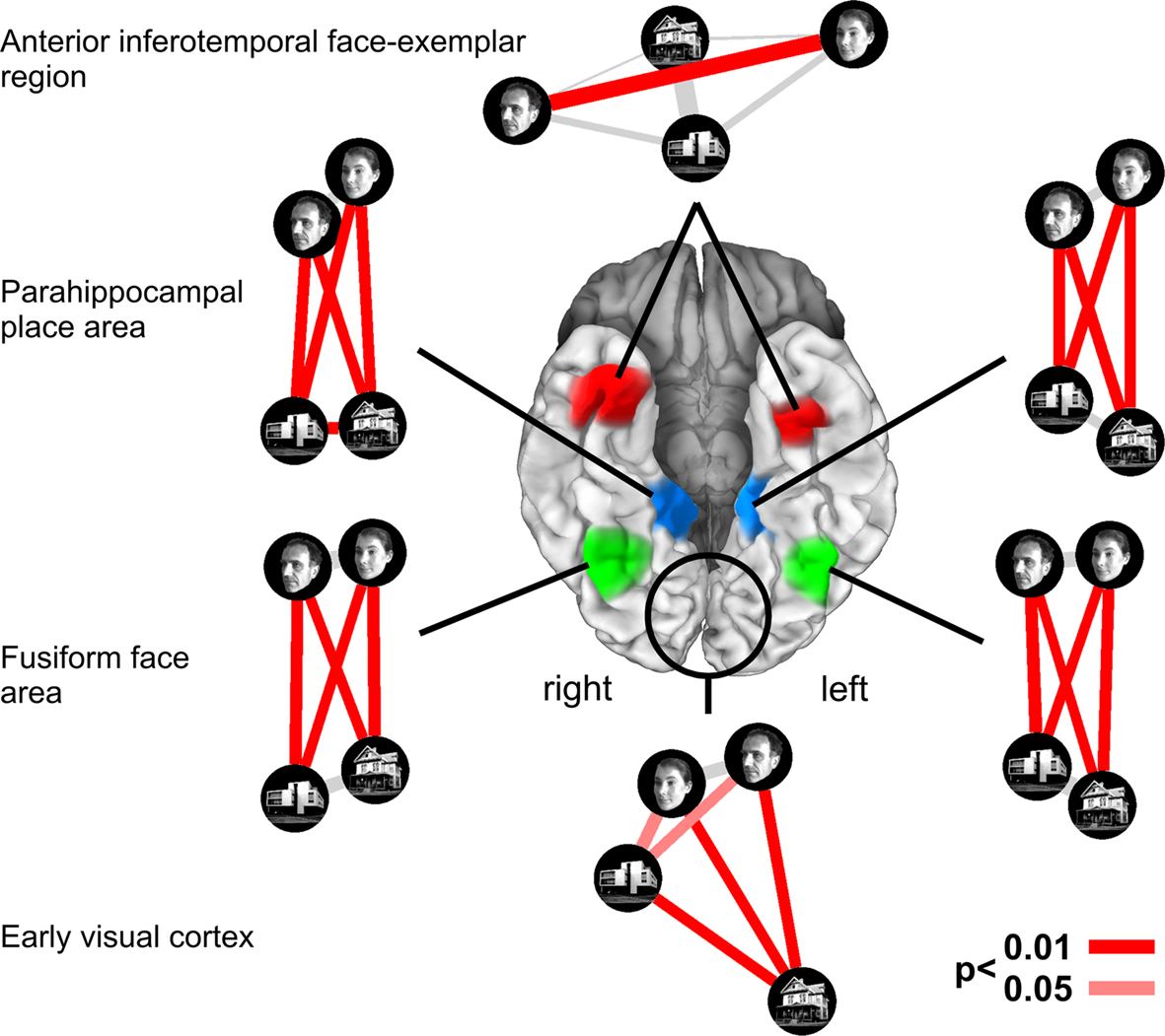
Figure 1. Characterizing brain regions by representational similarity structure. For each region, a similarity-graph icon shows the similarities between the activity patterns elicited by four stimulus images. Images placed close together in the icon elicited similar response patterns. Images placed far apart elicited dissimilar response patterns. The color of each connection line indicates whether the response-pattern difference was significant for the group (red: p < 0.01; light gray: p ≥ 0.05, not significant). A connection line, like a rubberband, becomes thinner when stretched beyond the length that would exactly reflect the dissimilarity it represents. Connections also become thicker when compressed. Line thickness, thus, indicates the inevitable distortion of the 2D representation of the higher-dimensional similarity structure. The thickness of the connection lines is chosen such that the area of each connection (length times thickness) precisely reflects the dissimilarity measure. This novel visualization of fMRI response-pattern information combines (A) a multidimensional-scaling arrangement of activity-pattern similarity (as introduced to fMRI by Edelman et al., 1998
), (B) a novel rubberband-graph depiction of inevitable distortions, and (C) the results of statistical tests of a pattern-information analysis (for details on the test, see Kriegeskorte et al., 2007
). The icons show fixed-effects group analyses for regions of interest individually defined in 11 subjects. Early visual cortex was anatomically defined; all other regions were functionally defined using a data set independent of that used to compute the similarity-graph icons and statistical tests.
The Representational Dissimilarity Matrix
For a given brain region, we interpret (Dennett, 1987
) the activity pattern associated with each experimental condition as a representation (e.g., a stimulus representation)
1
. By comparing the activity patterns associated with each pair of conditions (Edelman et al., 1998
; Haxby et al., 2001
), we obtain a representational dissimilarity matrix (RDM; Figure 2
), which serves to characterize the representation
2
.
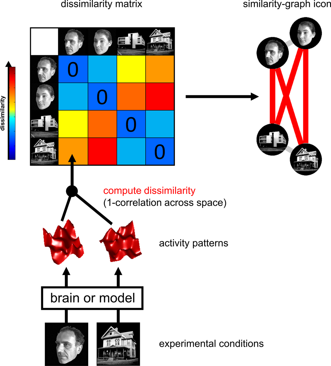
Figure 2. Computation of the representational dissimilarity matrix. For each pair of experimental conditions, the associated activity patterns (in a brain region or model) are compared by spatial correlation. The dissimilarity between them is measured as 1 minus the correlation (0 for perfect correlation, 1 for no correlation, 2 for perfect anticorrelation). These dissimilarities for all pairs of conditions are assembled in the RDM. Each cell of the RDM, thus, compares the response patterns elicited by two images. As a consequence, an RDM is symmetric about a diagonal of zeros. To visualize the representation for a small number of conditions, we suggest the similarity-graph icon (top right, cf. Figure 1
).
An RDM contains a cell for each pair of experimental conditions (Figure 2
). Each cell contains a number reflecting the dissimilarity between the activity patterns associated with the two conditions. As a consequence, an RDM is symmetric about a diagonal of zeros. We suggest using correlation distance (1-correlation) as the dissimilarity measure, although we explore a number of measures below (Figure 10
).
The RDM indicates the degree to which each pair of conditions is distinguished. It can thus be viewed as encapsulating the information content (in an informal sense) carried by the region. For any computational model (Figure 5
) that can be exposed to the same experimental conditions (e.g., presented with the same stimuli), we can obtain an RDM for each of its processing stages in the same way as for a brain region (Figure 6
).
The RDMs serve as the signatures of regional representations in brains and models. Importantly, these signatures abstract from the spatial layout of the representations. They are indexed (horizontally and vertically) by experimental condition and can thus be directly compared between brain and model. What we are comparing, intuitively, is the represented information, not the activity patterns themselves.
Matching Dissimilarity Matrices: A Second-Order Isomorphism
RDMs can be quantitatively compared just like activity patterns, e.g., using correlation distance (1-correlation) or rank-correlation distance. Because RDMs are symmetric about a diagonal of zeros, we will apply these measures using only the upper (or equivalently the lower) triangle of the matrices.
Analysis of similarity structure has a history in psychology and related fields. When exposed to a suitable sensory stimulus, our brain activity reflects many properties of the stimulus. The reflection of a stimulus property in the activity level of a neuron constitutes what has been termed a first-order isomorphism between the property and its representation in the brain. Most neuroscientific studies of brain representations have focused on the relationship between stimulus properties and brain-activity level in single cells or brain regions, i.e., on the first-order isomorphism between stimuli and their representations. One concept at the core of our approach is that of second-order isomorphism (Shepard and Chipman, 1970
), i.e., the match of dissimilarity matrices.
When we encounter difficulty establishing a direct correspondence, i.e., a first-order isomorphism
3
, in studying the relationship between stimuli and their representations, we may attempt instead to establish a correspondence between the relations among the stimuli on the one hand and the relations among their representations on the other, i.e., a second-order isomorphism. We can study the second-order isomorphism by relating the similarity structure of the objects to the similarity structure of the representations. This promises a higher-level functional perspective, which is complementary to the perspective of first-order isomorphism.
Related Approaches in the Literature
The qualitative and quantitative analysis of similarity structure has a long history in philosophy, psychology, and neuroscience. A good entry to the literature is provided by Edelman (1998)
, who (Edelman et al., 1998
) also pioneered application of similarity analysis to fMRI activity patterns using the technique of multidimensional scaling (MDS; Borg and Groenen, 2005
; Kruskal and Wish, 1978
; Shepard, 1980
; Torgerson, 1958
). Laakso and Cottrell (2000)
compared representations in hidden units of connectionist networks by correlating the dissimilarity structures of their activity patterns. They suggest that this approach could be used as a general method for comparing representations and discuss the philosophical implications. Op de Beeck et al. (2001)
related the representational similarity of silhouette shapes in monkey inferior temporal cortex to physical and behavioral similarity measures for those stimuli.
At a more general level, activity-pattern similarity is related to activity-pattern information as targeted in a number of recent studies in human fMRI (Carlson et al., 2003
; Cox and Savoy, 2003
; Davatzikos et al., 2005
; Friston et al., 2008
; Hanson et al., 2004
; Haxby et al., 2001
; Haynes and Rees, 2005a
,b
; Haynes et al., 2007
; Kamitani and Tong, 2005
, 2006
; Kriegeskorte et al., 2006
; LaConte et al., 2005
; Mitchell et al., 2004
; Mourao-Miranda et al., 2005
; Pessoa and Padmala, 2006
; Polyn et al., 2005
; Serences and Boynton, 2007
; Spiridon and Kanwisher, 2002
; Strother et al., 2002
; Williams et al., 2007
; for reviews see Haynes and Rees, 2006
; Kriegeskorte and Bandettini, 2007
; Norman et al., 2006
) and also in monkey electrophysiology (Hung et al., 2005
; Tsao et al., 2006
).
Explicit similarity analyses of neuronal activity patterns have begun to be applied in human fMRI (Aguirre, 2007
; Aguirre et al., in preparation
; Drucker and Aguirre, submitted
; Edelman et al., 1998
; Kriegeskorte et al., in press
; O’Toole et al., 2005
) and monkey electrophysiology (Kiani et al., 2007
; Op de Beeck et al., 2001
).
Connecting the Branches of Systems Neuroscience
In this paper, we argue that the theoretical concept of second-order isomorphism (Shepard and Chipman, 1970
) can serve a much more general purpose than previously thought, relating not only external objects to their brain representations, but bridging the divides between the three branches of systems neuroscience: behavioral experimentation, brain-activity experimentation, and computational modeling (Figure 3
).
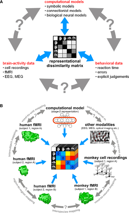
Figure 3. The representational dissimilarity matrix as a hub that relates different representations. (A) Systems neuroscience has struggled to relate its three major branches of research: behavioral experimentation, brain-activity experimentation, and computational modeling. So far these branches have interacted largely on two levels: (1) They have interacted on the level of verbal theory, i.e., by comparing conclusions drawn from separate analyses. This level is essential, but it is not quantitative. (2) They have interacted at the level characteristic functions, e.g., by comparing psychometric and neurometric functions. This form of bringing the branches in touch is equally essential and can be quantitative. However, characteristic functions typically contain only a small number of data points, so the interface is not informationally rich. Note that the RDM shown is based on only four conditions, yielding only (42 − 4)/2 = 6 parameters. However, since the number of parameters grows as the square of the number of conditions, the RDM can provide an informationally rich interface for relating different representations. Consider for example the 96-image experiment we discuss, where the matrix has (962 − 96)/2 = 4,560 parameters. (B) This panel illustrates in greater detail what different representations can be related via the quantitative interface provided by the RDM. We arbitrarily chose the example of fMRI to illustrate the within-modality relationships that can be established. Note that all these relationships are difficult to establish otherwise (gray double arrows).
We introduce an analysis framework called representational similarity analysis (RSA), which builds on a rich psychological and mathematical literature (Edelman, 1995
, 1998
; Edelman and Duvdevani-Bar, 1997a
,b
; Kruskal and Wish, 1978
; Laakso and Cottrell, 2000
; Shepard, 1980
; Shepard and Chipman, 1970
; Shepard et al., 1975
; Torgerson, 1958
). The core idea is to use the RDM as a signature of the representations in brain regions and computational models. We define a specific working prototype of RSA and discuss the potential of this approach in its full breadth:
(1) Integration of computational modeling into the analysis of brain-activity data. A key advantage of RSA is that computational models of brain information processing form an integrated component of data analysis and can be directly evaluated and compared. We demonstrate how to apply multivariate analysis to a set of dissimilarity matrices from brain regions and models in order to find out (1) which model best explains the representation in each brain region and (2) to what extent representations among regions and models resemble each other. We introduce a randomization test of representational relatedness and a bootstrap technique for obtaining error bars on estimates of the goodness of fit of different models.
(2) Relating regions, subjects, species, and modalities of brain-activity measurement. We discuss how RSA can be used to quantitatively relate:
• representations in different regions of the same brain (“representational connectivity”),
• corresponding brain regions in different subjects (“intersubject information”),
• corresponding brain regions in different species (e.g., humans and monkeys),
• and different modalities of brain-activity data (e.g., cell recordings and fMRI).
(3) Relating brain and behavior. We discuss how RSA can quantitatively relate brain-activity measurements to behavioral data. This possibility has already been demonstrated in previous work (Aguirre et al., in preparation
; Kiani et al., 2007
; Op de Beeck et al., 2001
).
(4) Addressing a broader array of neuroscientific questions with each experiment by means of condition-rich design. While RSA is applicable to conventional experimental designs, is synergizes with novel condition-rich experimental designs, where a single experiment can address a large number of neuroscientific questions. We demonstrate this with an fMRI experiment that has 96 separate conditions and discuss the broader implications.
We hope that RSA will contribute to a more integrated systems neuroscience, where different multi-channel measures of neural activity are quantitatively related to each other and to computational theory and behavior via the information-rich characterization of distributed representations provided by the RDM.
In this section we describe the core of RSA step-by-step. We assume that the data to be analyzed consists in a multivariate activity pattern measured for each of a set of conditions in a given brain region, whose representation is to be better understood. The data could be from single-cell or electrode-array recordings, from neuroimaging, or any other modality of brain-activity measurement. We demonstrate the analysis on an fMRI experiment, in which human subjects viewed 96 particular object images. The step-by-step description that follows describes the method. The empirical results for our example experiment are described and interpreted subsequently.
Step 1: Estimating the Activity Patterns
The first step of the analysis is the estimation of an activity pattern associated with each experimental condition. In our example, the activity patterns are spatial response patterns from early visual cortex (EVC) and from the fusiform face area (FFA). The analysis proceeds independently for each region.
Instead of spatial activity patterns we could use spatiotemporal patterns or simply temporal patterns from a single site as the input to RSA. Similarly, we could filter the measurements in some neuroscientifically meaningful way. For cell recordings, for example, we could use windowed spike counts, multi-unit activity, or local field potentials as the input.
In our fMRI example, we obtain an activity estimate for each voxel and condition using massively univariate linear modeling (Figure 7
). The design matrix used to model each voxel’s response is based on the event sequence and a linear model of the hemodynamic response (Boynton et al., 1996
). For each region of interest, the resulting condition-related activity patterns form the basis for computation of the representational dissimilarities.
Step 2: Measuring Activity-Pattern Dissimilarity
In order to compute the RDM (Figure 2
), we compare the activity patterns associated with each pair of conditions. A useful measure of activity-pattern dissimilarity that normalizes for both the mean level of activity and the variability of activity is correlation distance, i.e., 1 minus the linear correlation between patterns (cf. Aguirre, 2007
; Haxby et al., 2001
; Kiani et al., 2007
). Alternative measures include the Euclidean distance (cf. Edelman et al., 1998
), the Mahalanobis distance (cf. Kriegeskorte et al., 2006
) and, in order to relate RSA to conventional activation-based fMRI analysis, the absolute value of the regional-average activation difference (Figure 10
).
The dissimilarity values for all pairs of conditions are assembled in an RDM, which will have a width and height corresponding to the number of conditions and is symmetric about a diagonal of zeros (Figure 2
). We can use MDS to visualize the similarity structure of the activity patterns. This is demonstrated in Figure 4
, where conditions are represented by colored dots. The distances between the dots approximate the dissimilarities of the activity patterns the conditions are associated with.
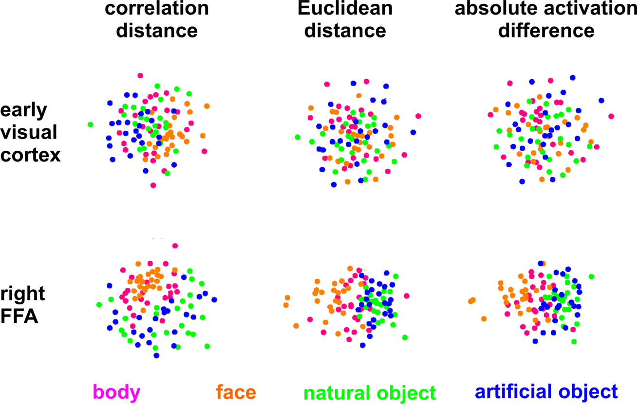
Figure 4. Unsupervised arrangement of 96 experimental conditions reflecting pairwise activity-pattern similarity. As in Figure 1
, but for 96 instead of 4 conditions, the arrangements reflect the activity-pattern similarity structure. Each panel visualizes the RDM from the corresponding panel in Figure 10
. Each condition (corresponding to the presentation of one of 96 object images) is represented by a colored dot, where the color codes for the category (legend at the bottom). In each panel, dots placed close together indicate that the two conditions were associated with similar activity patterns. Dots placed far apart indicate that the two conditions were associated with dissimilar activity patterns. The panels show results of non-metric multidimensional scaling (minimizing the loss function “stress”) for two brain regions (rows) and three activity-pattern dissimilarity measures (columns). Note that a categorical clustering of the face-image response patterns is apparent in the right FFA (bottom row), but not in early visual cortex (top row). (Note that the absolute activation differences could be represented by an arrangement along a straight line, had the dissimilarity matrices not been averaged across subjects.)
Step 3: Predicting Representational Similarity with a Range of Models
In this section we describe the different types of model that can be evaluated using RSA. Figure 5
shows the internal representations of several example models and Figure 6
shows the dissimilarity matrices characterizing the model representations.
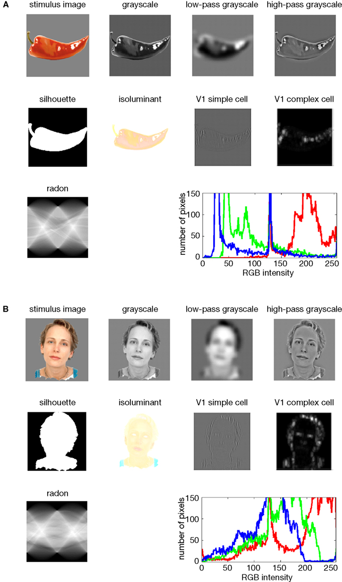
Figure 5. Model representations of two example images. Two example images (A,B) from the 96-image experiment and their representations in a number of computational models, including standard transformations of image processing as well as neuroscientifically motivated models. Note that each such representation defines a unique similarity structure for the 96 stimuli (as encapsulated in the RDMs of Figure 6
).
In order to evaluate a computational model with RSA, the model needs to simulate some aspect of the information processing occurring in the subject’s brain during the experiment. The term model, thus, has a different meaning here than conventionally in statistical data analysis, where it often refers to a statistical model that does not simulate brain information processing (such as the design matrix in Figure 7
, which was used to estimate the activity patterns).
In our example, we are interested in visual object perception, so the models to be used simulate parts of the visual processing. The models are presented with the same experimental stimuli as our human subjects. Moreover, their internal representations are analyzed in the same way as the measured brain representations of our subjects.
We demonstrate RSA with three complex computational models. First, we use a model of V1 consisting in retinotopic maps of simulated simple and complex cells based on banks of Gabor filters for a range of spatial frequencies and orientations at each location (details in the Appendix). We also include a variant of this model, in which we attempted to simulate the local averaging of fMRI voxels by pooling local responses of the original V1 model (V1 model, smoothed).
Second, as an example of a higher-level representation, we use a model developed in the HMAX framework (Riesenhuber and Poggio, 2002
; Serre et al., 2007
), which includes C2 units based on natural-image patches as filters and corresponds, approximately, to the level of representation in V4.
Third, we use a computational model from computer vision, the RADON transform, whose components in the present implementation are not meant to resemble neurons in the primate visual system. However, this model could be implemented with biological neurons and has been proposed as a functional account of the representation of visual stimuli in the lateral occipital complex (Wade and Tyler, 2005
) based on fMRI evidence. Detailed descriptions of the model representations are to be found in the Section “Methodological Details.”
Simple computational models
The models described above are meant to simulate brain information processing in some sense. We can additionally use simple image transformations as competing computational models. Although there may be no compelling neuroscientific motivation for such models, they can provide useful benchmarks and help us characterize the information represented in a given brain region. Here we include (1) the digital images themselves in the Lab color space (which more closely reflects human color similarity perception than the RGB color space more commonly used for image storage), (2) the luminance patterns (grayscale versions) of the images, (3) low-pass (i.e., smoothed), and (4) high-pass (i.e., edge-emphasized) versions of the luminance patterns, (5) the Lab joint histograms of the images (representing the set of colors present in each image), and (6) the silhouettes of the objects, in which each figure pixel is 1 and each background pixel 0. These models as well are described in more detail in the Appendix.
Conceptual models
Model dissimilarity matrices can be obtained not only from explicit computational accounts. A theory may specify that a given brain region represents particular information and abstracts from other information without specifying how the representation is computed. In such “conceptual models”, the information processing is miraculous (i.e., unspecified) and the activity patterns unknown. However, we can still specify a hypothetical similarity structure to be tested by comparison to the similarity structures found in different brain regions.
Here we use two categorical models as examples of this model variety (Figure 6
). The first is the animate–inanimate model, in which two object images are identical (dissimilarity = 0) if they are either both animate or both inanimate, and different (dissimilarity = 1) if they straddle the category boundary. The second categorical model follows the same logic for the category of faces: two object images are identical (dissimilarity = 0) if they are either both faces or both non-faces, and different (dissimilarity = 1) if exactly one of them is a face.
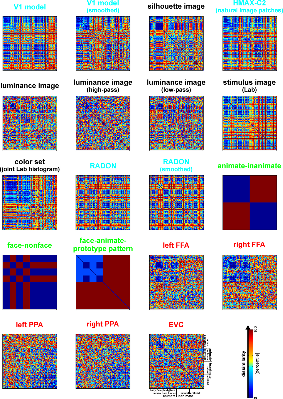
Figure 6. Representational dissimilarity matrices for models and brain regions. Dissimilarity matrices for model representations and regional brain representations (as introduced in Figure 2
). The dissimilarity measure is 1 − correlation (Pearson correlation across space). Note that each model yields a unique representational similarity structure that can be compared to that of each brain region (bottom five matrices). This comparison is carried out quantitatively in the following figure. The text labels indicate the representation depicted with the color indicating the type: complex computational model (blue), simple computational model (black), conceptual model (green), brain representation (red).
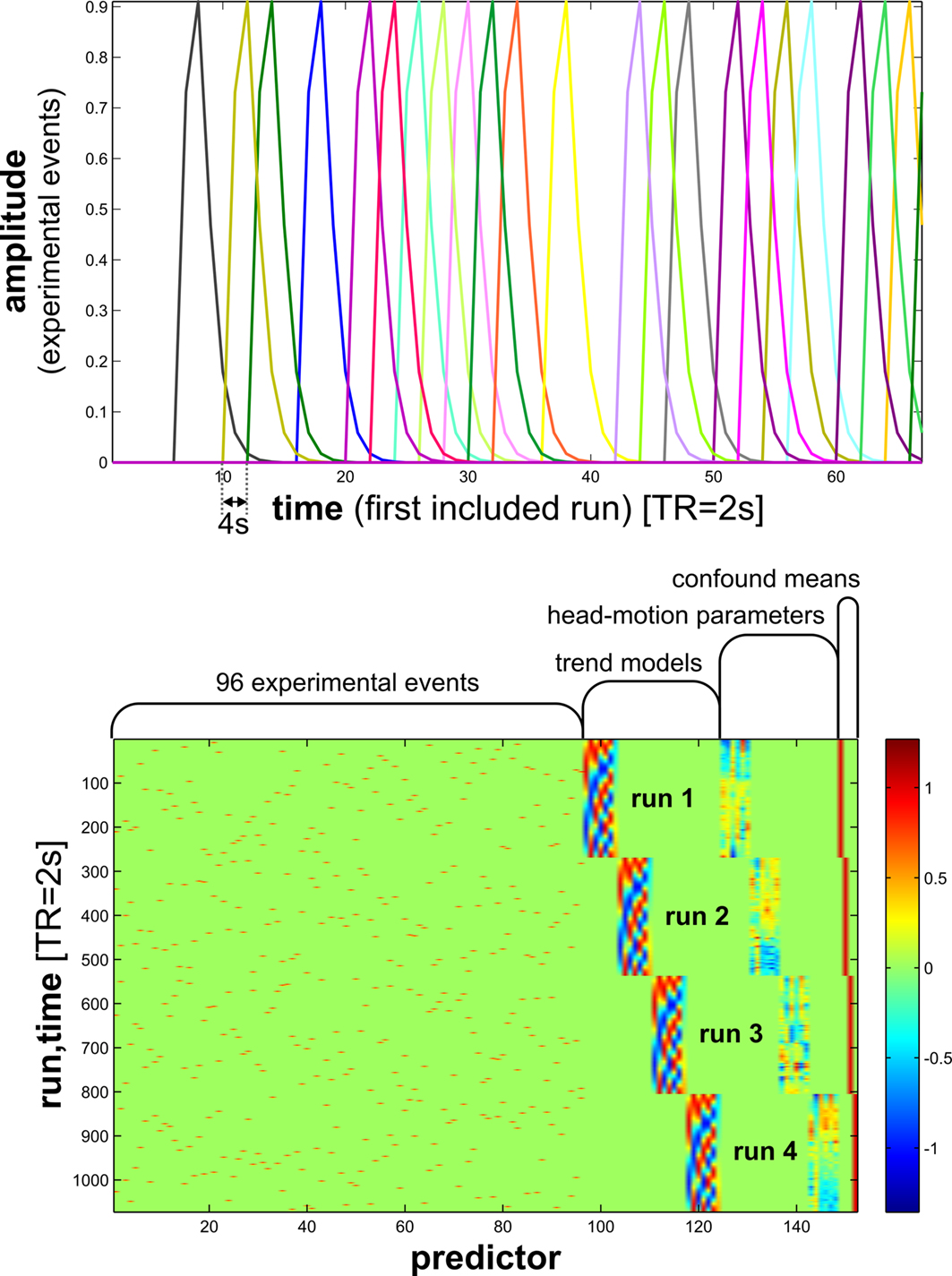
Figure 7. Design matrix for condition-rich ungrouped-events fMRI design. Both panels illustrate the design matrix used for the 96-image experiment, an example of a condition-rich ungrouped-events design. The top panel shows the hemodynamic predictor time courses for the experimental events occurring in the first couple of minutes of the first run. Note that events occur at 4-s trial-onset asynchrony, yielding overlapping but dissociable hemodynamic responses and a reasonable frequency of stimulus presentation. (Each of the 96 conditions occurs exactly once in each run. The condition sequence is independently randomized for each run.) The bottom panel shows the complete design matrix with predictor amplitude color coded (see colorbar on the right). In addition to the 96 predictors for the experimental conditions, the design matrix also includes components modeling slow artefactual trends and residual head-motion artefacts (after rigid-body head-motion correction), and a confound-mean predictor for each run.
In addition, we use a “face-animal-prototype model”, which assumes that all faces elicit a prototypical response pattern (implying small dissimilarities between individual face representations) and that the same is true to a lesser degree for the more general class of animal images.
Behavior-based similarity structure
We could also use behavioral measures to define reference dissimilarity matrices. The dissimilarity values could come from explicit similarity judgments or from reaction times or confusion errors in comparison tasks (Aguirre et al., in preparation
; Cutzu and Edelman, 1996
, 1998
; Edelman et al., 1998
; Kiani et al., 2007
; Op de Beeck et al. 2001
; Shepard et al., 1975
). Such behavioral dissimilarity matrices may reflect the representations that determine the behavioral choices, reaction times, or confusion errors. A close match between the RDM of a brain region and the behavioral dissimilarity matrix would suggest that the regional representation might play a role in determining the behavior measured.
Step 4: Comparing Brain and Model Dissimilarity Matrices
Once the dissimilarity matrices of the brain representations (Figure 10
) and those of theoretical models (Figure 6
) have been specified they can be visually and quantitatively compared. One way to quantify the match between two dissimilarity matrices is by means of a correlation coefficient. We use 1-correlation as a measure of the dissimilarity between RDMs (Figure 8
). Because dissimilarity matrices are symmetrical about a diagonal of zeros, the correlation is computed over the values in the upper (or equivalently the lower) triangular region. Note that above we suggested the use of this measure for comparing activity patterns. Here we suggest using it to assess second-order dissimilarity: the dissimilarity of dissimilarity matrices.
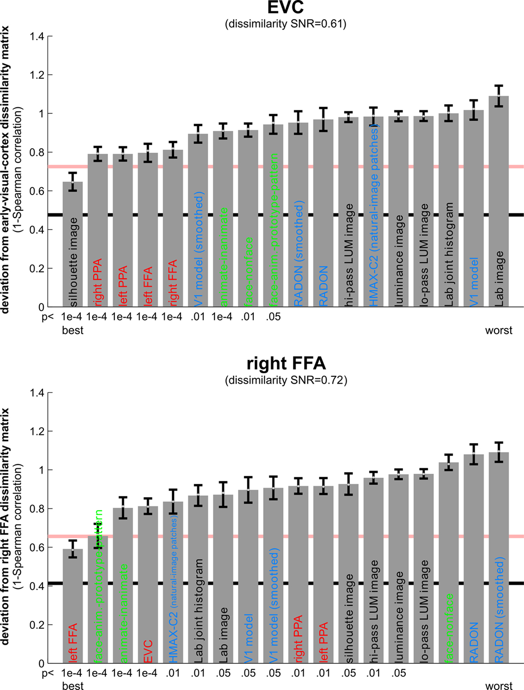
Figure 8. Matching models to brain regions by comparing representational dissimilarity matrices. The dissimilarity matrices characterizing the representation in early visual cortex (top) and the right FFA (bottom) are compared to dissimilarity matrices obtained from model representations and other brain regions. Each bar indicates the deviation between the RDM of the reference region (early visual cortex or the right FFA) and that of a model or other brain region. The deviation is measured as 1 minus the Spearman correlation between dissimilarity matrices (for motivation see Step 4 and Appendix). Text-label colors indicate the type of representation: complex computational model (blue), simple computational model (black), conceptual model (green), brain representation (red). Error bars indicate the standard error of the deviation estimate. (The standard error is estimated as the standard deviation of 100 deviation estimates obtained from bootstrap resamplings of the conditions set.) The number below each bar indicates the p-value for a test of relatedness between the reference matrix (early visual cortex or the right FFA) and that of the model or other region. (The test is based on 10,000 randomizations of the condition labels.) The black line indicates the noise floor, i.e., the expected deviation between the empirical reference RDM (with noise) and the underlying true RDM (without noise). The red line indicates the expected retest deviation between the empirical dissimilarity matrices that would be obtained for the reference region if the experiment were repeated with different subjects (both matrices affected by noise). Both of these reference lines as well as the dissimilarity signal-to-noise ratios (dissimilarity SNR: below the titles) are estimated from the variability of the dissimilarity estimates across subjects.
We could use an alternative distance measure, such as the Euclidean distance, for comparing dissimilarity matrices. As for comparing activity patterns, we again prefer correlation distance, because it is invariant to differences in the mean and variability of the dissimilarities. For the models we use here, we do not wish to assume a linear match between dissimilarity matrices. We therefore use the Spearman rank correlation coefficient to compare them. In the Appendix, we present another argument for the use of rank-correlation distance (instead of the Pearson linear correlation distance or Euclidean distance) for comparing dissimilarity matrices. The argument is based on the observation that, in high-dimensional response spaces, a prominent component of the effect of activity-pattern noise on the dissimilarities can be accounted for by a monotonic transform.
Figure 8
shows the deviations (1-Spearman correlation) of the models from each brain region’s RDM. Smaller bars indicate better fits. In order to estimate the variability of each model deviation expected if a similar experiment were to be performed with different stimuli (from the same population of stimuli), we computed each model deviation 100 times over for bootstrap resamplings of the condition set (i.e., 96 conditions chosen with replacement from the original set of 96 on each iteration)
4
. This method is attractive, (1) because it requires few assumptions, (2) because only the dissimilarity matrices are needed as input, (3) because it is computationally less intensive than modeling the noise at a lower level, and (4) because it generalizes (to the degree possible given the experimental data) from the set of conditions actually used in the experiment to the population of conditions that the actual conditions can be considered a random sample of. This bootstrap procedure would also lend itself to testing whether one model fits the data better than another model, as discussed in the Appendix
5
.
Step 5: Testing Relatedness of Two Dissimilarity Matrices by Randomization
In order to decide whether two dissimilarity matrices are related, we can perform statistical inference on the RDM correlation. The classical method for testing correlations assumes independent measurements for the two variables. For dissimilarity matrices such independence cannot be assumed, because each similarity is dependent on two response patterns, each of which also codetermines the similarities of all its other pairings in the RDM.
We therefore suggest testing the relatedness of dissimilarity matrices by randomizing the condition labels. We choose a random permutation of the conditions, reorder rows and columns of one of the two dissimilarity matrices to be compared according to this permutation, and compute the correlation. Repeating this step many times (e.g., 10,000 times), we obtain a distribution of correlations simulating the null hypothesis that the two dissimilarity matrices are unrelated. If the actual correlation (for consistent labeling between the two dissimilarity matrices) falls within the top α × 100% of the simulated null distribution of correlations, we reject the null hypothesis of unrelated dissimilarity matrices with a false-positives rate of α. The p-value for each brain region’s relatedness to each model is given beneath the model’s bar in Figure 8
. They are conservative estimates based on 10,000 random relabelings, so the smallest possible estimate is 10−4.
Step 6: Visualizing the Similarity Structure of Representational Dissimilarity Matrices by MDS
MDS provides a general method for arranging entities in a low-dimensional space (e.g., the 2D of a figure on paper), such that their distances reflect their similarities: Similar entities will be placed together, dissimilar entities apart. In Figure 4
we used MDS to visualize the similarity structure of activity patterns in EVC and FFA. Here we suggest using MDS also to visualize the similarity structure of RDM.
We first assemble all pairwise comparisons between activity-pattern dissimilarity matrices in a dissimilarity matrix of dissimilarity matrices (Figure 9
A), using rank-correlation as the dissimilarity measure as suggested above. We then perform MDS on the basis of this second-order dissimilarity matrix.
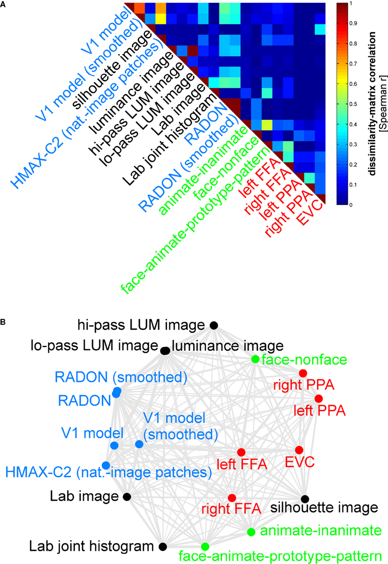
Figure 9. Simultaneously relating all pairs of representations. Figure 8
showed the relationships between two reference regions and all models and other regions. Here we simultaneously visualize the pair-relationships between all models and regions (text labels). Note that the visualization of all pair-relationships comes at a cost: statistical information is omitted here. Text-label colors indicate the type of representation: complex computational model (blue), simple computational model (black), conceptual model (green), brain representation (red). (A) The correlation matrix (Spearman rank correlation) of RDMs. (B) Multidimensional scaling arrangement (minimizing metric stress) of the representations. Note that MDS was used here to arrange not activity patterns (as in Figures 1 and 4
), but dissimilarity matrices. The rubberband graph (gray connections) depicts the inevitable distortions introduced by arranging the models in 2D (see legend of Figure 1
for an explanation).
This exploratory visualization technique (Figure 9
B) simultaneously relates all RDMs (from models and brain regions) to each other. It thus summarizes the information we would get by inspecting a bar graph of RDM fits (Step 4) not just for EVC and the right FFA (as shown in Figure 8
), but for each model and region. The conciseness of the MDS visualization comes at a cost: the distances are distorted (depending on the number of representations included) and there are no error bars or statistical indications. Nevertheless this exploratory visualization technique provides a useful overall view. It can alert us to relationships we had not considered and prompt confirmatory follow-up analysis.
The Representational Dissimilarity Matrices of EVC and FFA
Figure 10
shows that the correlation-distance matrix for EVC and FFA. For the FFA, but not EVC, the matrix reflects the categorical structure of the stimuli. This structure is obvious, because the condition sequence for the dissimilarity matrices were defined by the categorical order. Note, however, that this order affects merely the visual appearance of the matrices. Reordering the conditions does not affect the results of RSA. For the FFA, the correlation-distance matrix reveals a pattern markedly different from that exhibited by the two other measures of activity-pattern dissimilarity. The absolute-activation-difference matrix shows the prominent contrast in activation level between faces and inanimate objects and less prominently between animate and inanimate objects. The correlation-distance matrix normalizes out the regional-average activation effects and reveals that the activity patterns are highly correlated among faces (human or animal) and to a lesser degree among animals. The Euclidean-distance matrix is sensitive to both the absolute activation difference and the pattern correlation. Unless indicated otherwise, subsequent analyses are based on correlation-distance matrices.
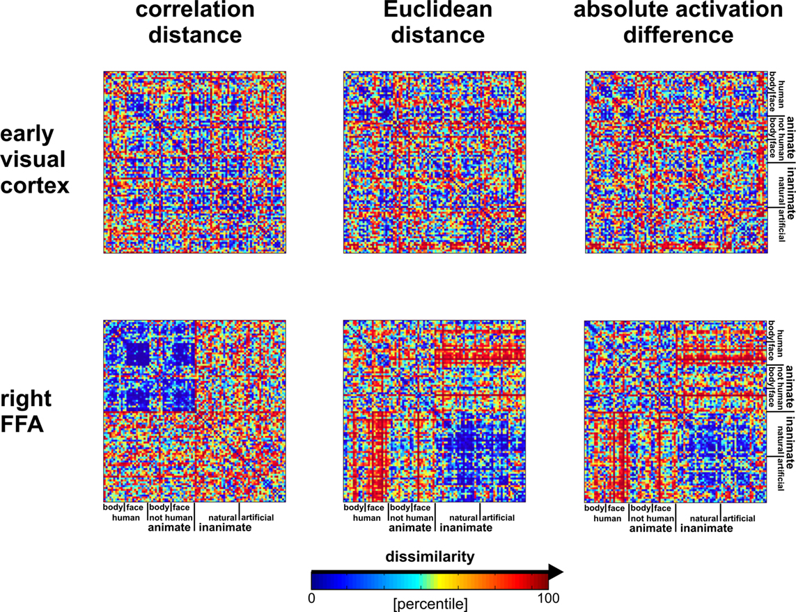
Figure 10. Dissimilarity matrices of activity patterns elicited in early visual cortex and FFA by viewing 96 object images. Dissimilarity matrices (as introduced in Figure 2
) are shown for early visual cortex (top row) and right FFA (bottom row) and for three different measures of dissimilarity (columns): 1 − correlation (Pearson correlation across space), the Euclidean distance between the two response patterns (in standard error units) and the absolute activation difference (i.e., the absolute value of the difference of the spatial-mean activity level). The absolute activation difference is sensitive only to the overall level of activation and has been included only because regional-average activation is conventionally targeted in fMRI analysis. Note that the correlation distance (1 − correlation) normalizes for both the overall activation and the variability of activity across space. It is therefore the preferred measure for detecting distributed representations without sensitivity to the global activity level (which could be attributed e.g., to attention). The Euclidean distance combines sensitivity to pattern shape, spatial-mean activity level, and variability across space. Note that as expected using the Euclidean distance yields an RDM resembling both the one obtained with correlation distance and the one obtained with absolute activation difference. The matrices have been separately histogram-equalized (percentile units) for easier comparison. Dissimilarity matrices were averaged across two sessions for each of four subjects.
The Similarity Structure of Activity Patterns in EVC and FFA as Revealed by MDS
Figure 4
visualizes the dissimilarity structure as estimated with the three measures by arranging dots that represent the 96 object images in 2D with category-color-coding, such that stimuli eliciting similar response patterns are placed close together and stimuli eliciting dissimilar response patterns are placed far apart. Such arrangements are computed by MDS. We observe some categorical clustering (for faces and, to a lesser degree, for animate objects) in FFA, but not in EVC. This is consistent with our inspection of dissimilarity matrices in Figure 10
.
Model Fits to EVC and FFA
Figure 6
shows the RDMs of the models. The first thing to note is that each matrix presents a unique pattern that characterizes the model representation. Figure 8
shows the deviation of each model from the empirical RDMs of EVC and FFA. We do not have the space here to fully discuss the neuroscientific implications of this analysis, but we offer some basic observations that demonstrate how RSA can help characterize regional representations:
• For EVC, note that the best-fitting model is the silhouette-image model. This is plausible because EVC is known to contain retinotopic representations of the visual input. The fMRI patterns in EVC appear to reflect primarily the shape of the retinotopic region stimulated (i.e., the shape of the figure, since the background is uniformly gray). That the simple silhouette model explains the RDM better here than the V1 model suggests that the orientation information is not as strongly reflected in the RDM. This is consistent with recent results by Kay et al. (2008)
, who showed that images can be identified on the basis of their fMRI responses in EVC, with the major portion of the information provided by the retinotopic representation of edge energy and a smaller portion provided by the representation of edge orientation
6
. Early visual orientation information is likely to be attenuated in fMRI data because of its fine-scale spatial organization and pooling of columns of all orientation-preferences in each fMRI voxel.
• Among the complex computational models, the V1 model fits the EVC data best, but only the “smoothed” version, where we simulated local pooling of orientation-specific responses in fMRI voxels. Like the good fit of the silhouette model, this is consistent with the limited spatial resolution of our fMRI voxels.
• The RDMs of the fusiform face and parahippocampal place areas in either hemisphere fit the EVC matrix better than the V1 model, but not as well as the silhouette model. One explanation for this is that the conventional V1 model does not capture the full complexity of the representation in EVC. This would be plausible for two reasons: On the one hand, our EVC region contains voxels from the early visual foveal confluence, not just from V1. On the other hand, V1 itself is likely to contain a more complex representation than our Gabor-based model of simple and complex cells.
• The higher-level HMAX-C2 representation based on natural image patches, plausibly does not capture the similarity structure we find in EVC, nor do the simple image transformations.
• For the right FFA, the best-fitting dissimilarity structure consists in the empirical dissimilarity of FFA in the opposite hemisphere. This is plausible, given the close functional relationship between the regions.
• The dissimilarities of the right FFA are best modeled by a conceptual model: the “face-animal-prototype model”. This suggests that, to a first approximation, different faces elicit a prototypical response pattern – implying small dissimilarities between individual face response patterns, consistent with Kriegeskorte et al. (2007)
, and that the same is true to a lesser degree for the more general class of animal images.
• Among the complex computational models, the HMAX-C2 representation based on natural image patches provides the best fit to the right FFA. This may reflect the higher-level nature of the representations in FFA.
• The right FFA resembles the EVC more closely than the V1 model, the silhouette model, or any other brain region. This could reflect feedback from FFA to EVC. Alternatively, FFA may reflect some of the more complex features of the early visual representation that are not captured by either the silhouette or the V1 model.
The Similarity Structure of Representational Dissimilarity Matrices as Revealed by MDS
Figure 9
simultaneously relates the RDM “signatures” of all brain regions and models to each other by means of MDS. This representation is devoid of indications of statistical significance and inevitably compromised by geometric distortions (because a higher-dimensional structure is represented in 2D). However, it provides a useful overview of all pairwise relationships (not just the relationships shown in Figure 8
of EVC and the right FFA to the other representations). Although the 2D distances do not precisely reflect the actual dissimilarities between the dissimilarity matrices, almost all observations from Figure 8
are also reflected in the MDS arrangement of Figure 9
. However, the MDS arrangement provides us with a lot of additional information. As examples of the additional information, consider these observations:
· The close interhemispheric observed for the left and right FFA (Figure 8
), also holds for the left and right parahippocampal place area.
· The smoothing applied to the V1 model and the RADON model in order to simulate pooling of responses within fMRI voxels does not appear to drastically alter the RDM of either of these models.
· The five brain regions included (red) all seem to be somewhat related in their representational similarity structure. The fact that no model appears in their midst suggests that there may be a common component to these visual representations that is not captured by any of the models.
Relating Models, Brain Regions, Subjects, Species, and Behavior
Systems neuroscience has struggled to quantitatively relate its three major branches of research: behavioral experimentation, brain-activity experimentation, and computational modeling. The RDM can serve as a hub that relates representations from a variety of sources in the three branches (Figure 3
). We can use dissimilarity matrices to compare internal representations between two models or two brain regions in the same subject (representational connectivity, see below). In addition, RSA provides a solution to the fine-grained spatial-correspondency problem encountered when relating corresponding brain regions in different subjects of an fMRI experiment. Conventionally, different subjects in an fMRI experiment are related by transforming the data into a common spatial frame of reference, such as Talairach space (Talairach and Tournoux, 1988
) or cortical-surface space defined by cortex-based alignment (Fischl et al., 1999
; Goebel and Singer, 1999
; Goebel et al., 2006
). However, these available common spaces do not have sufficient precision to relate high-resolution fMRI voxels. Establishing spatial correspondency is not merely a technical challenge. It is a fundamental empirical question to what spatial precision intersubject correspondency even exists in different functional areas (Kriegeskorte and Bandettini, 2007
). RSA offers an attractive way of abstracting from the spatial layout and even from the linear basis of the representation, allowing us to relate fine-grained activity patterns between subjects. Even different species and modalities of brain-activity data (e.g., single-cell recording and fMRI; Kriegeskorte et al., in press
) can be meaningfully related with RSA.
Advanced Types of Representational Similarity Analysis
RSA also allows us to localize a brain region whose intrinsic representation resembles that of a specified model. For this purpose we can move a spherical or cortex-patch searchlight (Kriegeskorte et al., 2006
) throughout the measured volume to select, at each location, a local contiguous set of voxels, for which RSA is performed. The results, for each model, form a continuous statistical brain map reflecting how well that model fits in each local neighborhood.
Representational connectivity analysis
In order to assess to what extent two brain regions in the same subject represent the same information, we can compare the two regions’ condition- or time-point-based dissimilarity matrices (Kriegeskorte et al., in press
). The latter approach can be applied to either the raw data or residuals of the linear modeling of stimulus-related effects. Using the residuals will focus the analysis on the internal representational dynamics of the system including stochastic innovations. In analogy to functional connectivity analysis, we refer to this approach as “representational connectivity analysis”. It can be combined with the searchlight approach (Kriegeskorte et al., 2006
) in order to find a set of regions representationally connected to a given region.
Fitting parameters of computational models
The computational models we present as examples here are fixed models in that they do not have any parameters fitted on the basis of the data. It will be interesting to extend our approach to the fitting of model parameters on the basis of an empirical RDM. For example, a network model could be trained (supervised learning) to fit a given RDM. In order to avoid circular (i.e., self-fulfilling) inference, a separate set of conditions (e.g., different experimental stimuli) will then be needed to assess the fit of the computational model to the experimental data.
Composite modeling of a brain region’s representational dissimilarity matrix
In our demonstration here, we have treated the models as separate accounts of the data to be evaluated independently. A complementary approach is to model the RDM of a brain region by combining several models. To this end, one could combine units from the internal representations of several models (as we have done for simple and complex V1-model units) and compute the overall representational dissimilarity. One could then fit parameters, including the number of units from each model to include in the representation, so as to best account for an empirical RDM. A simpler approach is to directly model an empirical RDM as a combination of model dissimilarity matrices. If we use Euclidean distance to compare activity patterns and assume that the different models account for orthogonal components of the activity patterns (e.g., separate sets of units), then we can account for the squared empirical Euclidean distance matrix as a linear combination of the squared model Euclidean distance matrices. (Note that this does not require the dissimilarity patterns of the models to be orthogonal; the linear model would use the dissimilarity variance uniquely explained by each model to disambiguate the explanation of shared dissimilarity variance.) A more generally applicable approach would be to explain the empirical RDM as a weighted sum of monotonically transformed model dissimilarity matrices, where a separate monotonic transform is estimated for each model simultaneously with the weights.
Weighted representational readout analysis
So far we have thought of a region’s representation as characterized by a single RDM. Alternatively, we can consider the representation as a high-dimensional structure that is viewed from different perspectives by the regions that read it out. If readout consists in multiple linear weightings of the representational units, then it amounts to a linear projection that can be likened to the transformation of a 3-D structure to a 2-D “view” of it. In this spirit, we can reverse the logic of the previous paragraph and see to what extent we can read out a particular dissimilarity structure from the representation by weighting the units before computing the RDM. Again, using the squared Euclidean distance yields a simple relationship: Each unit (e.g., a voxel or a neuron) yields a separate RDM. The overall squared Euclidean distance matrix is the sum of the single-unit squared Euclidean distance matrices. Now we can “account for” each model’s dissimilarity pattern as a linear combination of the single-unit dissimilarity matrices. This avenue can be construed as a generalization of linear discriminant analysis from a single contrast to a complex pattern of contrast predictions. It is interesting because of its neuroscientific motivation in terms of readout by other brain regions. As in linear discriminant analysis and classification in general, independent test data will be needed to confirm any relationships suggested by such a fit.
Core Concepts for Experimental Design
What experimental designs lend themselves to RSA? A distinguishing feature of RSA is its potential to simultaneously exploit the spatial and temporal richness of multi-channel brain-activity data. Although RSA can be applied to a wide range of conventional experimental designs, there may be little conceptual motivation for it in the context of certain experiments, e.g., a low-resolution block-design fMRI experiment that targets regional activation and averages across very different processes (e.g., perception of different stimuli within a given category). The benefits of RSA will be greatest for condition-rich experimental designs targeting activity-pattern information with high-resolution measurement. In this section we describe novel types of experimental design that are feasible with RSA and optimally exploit its potential.
Condition-rich design
RSA is particularly useful in conjunction with condition-rich designs. One example of such a design is the 96-object-image experiment we presented to demonstrate the approach. We refer to a design as condition-rich if the number of effective experimental conditions (that is brain states to be discerned) is large. Condition-rich designs approach the limit of the temporal complexity of the signal measured in order to amply sample the space of all possible conditions.
Within the classical approach of massively univariate activation-based analysis (Friston et al., 1994
, 1995
; Worsley and Friston, 1995
; Worsley et al., 1992
), one way of enriching design has been to parameterize the conditions. The result is a larger number of conditions that might not singly yield stable estimates, but the correlation between condition parameters and brain activity – combining evidence across conditions – can be stably estimated. Such designs also lend themselves to RSA: The model dissimilarity matrices can be computed from the condition parameters.
However, RSA is not limited to designs whose conditions sample a predefined parameter space in a regular way. In RSA, the parametric statistical models describing activity variation across time are replaced by computational models exposed to the same experimental conditions. Regular parameterization may help focus the experiment on particular hypotheses, but RSA also accommodates less restricted designs such as the 96-object-image design we use as an example here.
Ungrouped-events design
In the classical block-design approach to fMRI experimentation, an experimental block corresponding to one of the conditions typically includes a variety of brain states (e.g., corresponding to percepts of a variety of stimuli from the same category) that are to be averaged across. While differences between block-average activation can be very sensitively detected with this method, the average results will be ambiguous with respect to single-trial processing (Bedny et al., 2007
; Kriegeskorte et al., 2007
). Equally importantly, the temporal capacity of the fMRI signal to discern a large number of separate brain states is largely wasted. In event-related designs (Buckner, 1998
), stimuli can appear in complex temporal sequences allowing for a wider range of experimental tasks. However, the experimental events are usually still grouped in condition sets and the variety of events forming a single condition is averaged across in the analysis (e.g., by modeling each condition by a single predictor). The sequence of experimental events is often designed to maximize estimation efficiency for the condition contrasts of interest. In that case the design itself will imply a grouping of the experimental events.
We propose to avoid any predefined grouping of experimental events (ungrouped-events design). Each experimental event (e.g., each stimulus) is treated as a separate condition (Figure 7
; Aguirre 2007
; Kriegeskorte et al., 2007
; Kriegeskorte et al., in press
). The 4-image experiment is an example of an ungrouped-events design. The 96-image experiment is an example of an ungrouped events design, which is also condition-rich.
One approach is to have events occur in a random sequence implying no grouping. In order to include a reasonable number of events, but still be able to discern the activity patterns they are associated with, we use a design with temporally overlapping but still separable single-trial hemodynamic responses here. Our example employs a design with a trial-onset asynchrony (TOA) of 4 s (Figure 7
). The effects of varying the TOA are explored in Figure 11
. A more detailed discussion of optimal event sequences for condition-rich designs (including ungrouped-events designs) is to be found in the Appendix (Section “Optimal Condition-Rich fMRI Design”).

Figure 11. Design efficiency as a function of trial-onset asynchrony for a 96-condition fMRI design. This figure shows simulation results exploring how statistical efficiency depends on the trial-onset asynchrony (TOA) under linear-systems assumptions for a 96-condition design with one hemodynamic-response predictor per condition and a random sequence of experimental events (including 25% null events for baseline estimation). We assume that about 50 min of fMRI data are to be collected in a single subject. The simulation suggests a simple conclusion: The more closely the trials are spaced in time, the higher the efficiency will be (top panels) for single-conditions (cyan) and pairwise condition contrasts (red). Doubling the number of trials packed into the same 50-min period, then, would improve efficiency about as much as performing the whole experiment twice: decreasing the standard errors of the estimates roughly by a factor of sqrt(2). In other words, the standard errors are proportional to sqrt(TOA). (Why does not the greater response overlap decrease efficiency? For an intuitive understanding, consider that although the greater response overlap for shorter TOAs correlates predictors, the greater number of event repetitions decorrelates them.) Importantly, however, the straightforward relationship suggested by the simulation rests on the assumption of a linear neuronal and hemodynamic response system. In reality, the effects of closely spaced events may interact at the neuronal level and the hemodynamic responses may also not behave linearly (e.g., three 16-ms stimuli at a TOA of 32-ms are unlikely to elicit a hemodynamic response that is three times higher than that to a single such stimulus). The choice of TOA therefore requires an informed guess regarding the short-TOA nonlinearity for the particular experimental events used. For the 96-image experiment, we chose a TOA of 4 s. Details on the simulation and an intuitive explanation for the result are given in the Appendix (Section “Optimal Condition-Rich fMRI Design”), along with further discussion of design choices including the TOA.
For estimation of a given contrast of interest, a condition-rich ungrouped-events design with a random sequence will be less efficient than a block-design or a sequence-optimized rapid event-related design. In our view, however, the statistical cost is more than offset by the ability to group the events into arbitrary sets and, more generally, to study the rich space they populate and its relationship to the brain-activity patterns they are associated with. RSA provides an attractive method for exploring this rich empirical information and testing particular hypotheses.
Unique-events design and time-continuous experimentation
An ungrouped-events design does not group different experimental events into a condition set, but it may contain repetitions of identical experimental events. An extreme type of ungrouped-events design would be a unique-events design, in which no experimental event is ever repeated. RSA can handle unique-events designs just like any other design. This is an important property, because unique-events designs take the complexity of the conditions set to the limit of the temporal capacity of the measured signal. In addition, there are neuroscientific domains, where exact repetition of an experimental event is a questionable concept. Strictly speaking each experimental event in any experiment – and in fact any experienced event at all – permanently changes the brain. In many studies, we may choose a design that minimizes such effects so that we can neglect them in the analysis. For studies of plasticity, however, it may be attractive to track changes to the system along with its activity dynamics. RSA in conjunction with a suitably plastic computational model could address this challenge.
We can go one step further and abolish the notion of discrete experimental events in favor of that of time-continuous experimentation (e.g., Hasson et al., 2004
). For time-continuous designs, we can treat each acquired volume as a separate condition and directly compute the RDM from the data. For each region of interest, the resulting RDM will then have a width and height corresponding to the number of time points. We refer to such a dissimilarity matrix as a time2 dissimilarity matrix. For fMRI data, the time2 dissimilarity matrix will reflect the temporal characteristics of the hemodynamic response.
Time-continuous RSA is attractive for studies of time-continuous perception of stimuli, including complex natural stimuli such as movies (Hasson et al., 2004
), and, more generally, for studies of time-continuous interactions, such as playing computer games or interacting with a virtual-reality environment (Baumann et al., 2003
). Note that time-continuous experimentation allows for greater ecological validity (i.e., the subject’s experimental experience can be made more similar to experiences in natural environments). However, time-continuous experimentation can also utilize stimuli and interactions that are unnatural and designed to address a particular hypothesis – trading ecological validity for experimental control.
Data-Driven and Hypothesis-Driven Representational Similarity Analysis
RSA lends itself to a broad spectrum of analyses from data-driven (where results richly reflect the data) to hypothesis-driven (where results are strongly constrained by theoretical assumptions and the data serve to test predefined hypotheses). On the former end of the spectrum, the RDM itself richly reflects a given region’s representation. A multidimensional-scaling arrangement of the conditions set in 2D (Figures 1 and 4
) provides a data-driven, exploratory visualization that can allow us to discover natural groupings within the representational space (Edelman et al., 1998
). But RSA becomes distinctly hypothesis-driven when we test whether a predefined model fits a brain region’s representation (Figure 8
). One hallmark of hypothesis-driven analysis is complexity reduction. When we test a model fit by comparing two dissimilarity matrices, the voxel-by-time data matrix is reduced to a single fit parameter or the result of a statistical test.
The RDM at the front end of RSA certainly is a more data-driven representation than a scalar measure of model fit. But how rich is it exactly? That depends on the number of conditions. Usually computing the RDM will reduce the amount of data. Consider a single-subject experiment with 96 conditions (as in our example here). Let’s assume we are analyzing a region of 100 voxels and the experiment has 500 time points. The data matrix has 100 × 500 = 50,000 numbers. The RDM (symmetrical about a diagonal of zeros) has (962 − 96)/2 = 4,560 parameters. Computing the RDM, thus, constitutes a complexity reduction. If we consider the time2 dissimilarity matrix, on the other hand, we have expanded the data matrix into a 500 × 500 matrix with (5002 − 500)/2 = 124,750 parameters.
Meaningful statistical summaries
In order to learn from the massive amounts of brain-activity data we can acquire today with techniques including fMRI as well as scalp and invasive multi-channel electrophysiological techniques and voltage-sensitive dye imaging, we need meaningful statistical summaries that relate a complex data set to systems-level theory. First, statistical summaries are needed to reduce the complexity of the effects and relate them to theory. Second, statistical summaries combine the evidence of many noisy measurements, thus helping us separate effects from noise.
The most obvious and widespread method of summarizing data is averaging. While potentially powerful, averaging applied too early in the analysis can remove the effects of greatest neuroscientific interest. In fMRI, for example, data are often locally averaged (i.e., smoothed) prior to mapping analysis. This removes fine-grained spatial-pattern effects that reflect each functional region’s intrinsic representation (Kriegeskorte and Bandettini, 2007
; Kriegeskorte et al., 2006
). Similarly in the temporal dimension, grouped-events designs (including block designs) average across very different experimental events, rendering results ambiguous with regard to single-trial processing (Bedny et al., 2007
; Kriegeskorte et al., 2007
).
Late combination of evidence
A central theme of RSA is late combination of evidence: In order to better exploit the complexity of the data toward neuroscientific insights, spatial as well as temporal averaging (across sets of different experimental events) is omitted. This does not mean that the analysis involves less combination of evidence for reduction of complexity. Instead the combination of the evidence occurs later on, in ways that are conceptually better motivated.
Evidence is combined in RSA, for example, when (1) the patterns of activity within an extended region of interest are summarized in an RDM, when (2) dissimilarity matrices for a given functional region are averaged across subjects, and when (3) the complex structure of the resulting group-average RDM is compared to model dissimilarity matrices (summarizing the region’s function by its goodness of fit to several models or by the index of the best-fitting model).
Combining evidence requires theoretical assumptions. If we take a step back to look at the empirical cycle as a whole, we can motivate late combination of evidence in terms of late commitment to theoretical assumptions.
Late commitment: Using theoretical assumptions to constrain analysis, not design
In the first step of the empirical cycle, we strive to minimize the theoretical assumptions built into the experimental design. This approach is motivated by the observation that designs, e.g., of fMRI experiments, can be made much more versatile (allowing us to address more neuroscientific questions) at moderate costs in terms of statistical efficiency (for addressing a given question). A general design that can address a 100 questions appears more useful than a restricted design that addresses a single question with slightly greater efficiency.
Statistical power is afforded by combining the evidence – usually by averaging. When we decide on a grouping of experimental events (e.g., for a block design), we commit to a particular way of combining the evidence and thus give up versatility. Ungrouped-events designs allow us to combine the evidence in many different ways during analysis. First, this approach allows for exploratory analyses, which can (1) test basic assumptions of a field, (2) usefully direct our attention to larger phenomena (in terms of explained variance), and (3) lead to unexpected discoveries. Second, ungrouped-events designs allow a broad set of theoretically constrained analyses to be performed on the same data. And third, as a consequence, such designs allow us to combine data across studies and research groups in order to address a particular question with a power otherwise unattainable. In the Appendix, we assess this third point, the potential of data sharing within subfields of neuroscientific inquiry, in detail.
To What Extent does Measured Pattern Information Reflect Neuronal Representations?
A fundamental question in systems neuroscience is to what extent brain-activity patterns measured with different techniques reflect neuronal pattern information. RSA characterizes pattern information in terms of pattern similarity and, thus, provides one attractive avenue for addressing this issue. We will focus our discussion here on blood-oxygen-level-dependent fMRI (Bandettini et al., 1992
; Kwong et al., 1992
; Ogawa et al., 1990
, 1992
), but similar arguments hold for other modalities.
What pattern information will be shared between fMRI and neuronal activity is difficult to predict, because fMRI voxels sample neuronal activity through a complex spatiotemporal transform: the hemodynamics. If voxels reflected simply the spatiotemporally local average of neuronal activity, then any neuronal pattern differences in the attenuated high spatial and temporal frequency bands would be reduced or eliminated in the fMRI similarity structures. However, fMRI voxel sampling is likely to be more complex than local averaging and may have sensitivity to neuronal pattern information in unexpectedly high spatial (and possibly temporal) frequencies (consider Kamitani and Tong, 2005
). The unexpected sensitivity of fMRI is encouraging, but also suggests a more complex transform from neuronal to fMRI patterns, making it more difficult to predict what aspects of neuronal information exactly are reflected in fMRI patterns.
We used RSA to relate neuronal patterns recorded in monkey IT (Kiani et al., 2007
) to fMRI patterns elicited by the same set of 92 object images (the set also used in our example here) in human IT (Kriegeskorte et al., in press
). Despite the confounding species difference, results show a surprising match between the two dissimilarity matrices (linear correlation = 0.49, p < 0.0001). This indicates not only that monkey and human IT represent similar object-image information, but also that this information is similarly reflected in single-cell recordings and high-resolution fMRI, when analyzed with massively multivariate information-based techniques. The convergence of fMRI and neuronal recordings had not previously been addressed at the level of pattern information and our results are encouraging. Ultimately, however, assessing to what extent pattern information is shared between neuronal activity and fMRI will require simultaneous measurement in both modalities, just as for local activity (Logothetis et al., 2001
; Shmuel et al., 2007
).
It appears likely that high-resolution fMRI (Cheng et al., 2001
; Duong et al., 2001
; Harel et al., 2006
; Hyde et al., 2001
; Kriegeskorte and Bandettini, 2007
; Yacoub et al., 2003
) and cell recording will turn out to convey overlapping but non-identical components of the underlying neuronal pattern information. While fMRI is limited by hemodynamic signal confluence yielding an ambiguous combination signal at each voxel, invasive electrophysiological techniques are limited by selective subsampling of neuronal responses. It will be interesting to see if fMRI provides us with merely a subset of the information recorded by implanted multi-electrode arrays or if it can also give us neuronal pattern information missing in a given array recording. RSA appears attractive for relating modalities and also for use in each modality, no matter what their relationship turns out to be.
Relation Between RSA and other Tools of Pattern-Information Analysis
Multivariate techniques of pattern-information analysis have recently gained momentum in fMRI and electrophysiology (see list of citations in the Section “Introduction”). RSA shares a key feature with the cited pattern-information approaches: it is motivated by the theoretical concept of distributed representation and targets activity-pattern information, combining evidence across space and time. However, RSA differs from the cited pattern-information approaches in that it considers how the activity-pattern dissimilarity matrix relates to dissimilarity matrices predicted by theoretical models, i.e., a second-order isomorphism. The cited pattern-information approaches, in contrast, attempt to demonstrate that each condition is associated with a distinct activity pattern, i.e., a first-order isomorphism.
RSA can be thought of as a particular variant of pattern-information analysis, which need not involve decoding or classification of internal representations. But at the same time RSA can be construed as a generalization of pattern-information analysis, where many pattern-contrast predictions are tested together. A test of the discriminability of the activity patterns associated with two conditions is handled as a special case, using a binary model dissimilarity matrix
7
.
An important feature of RSA is the goal of understanding and quantitatively explaining the empirical RDM. This entails a healthy focus on the major variance-explaining components in the data. In classifier-based pattern-information analysis, by contrast, we typically focus on a particular dimension defined by the sets of experimental conditions we set out to discriminate. Classifier-based pattern-information analysis, therefore, typically has a stronger theoretical bias than RSA. However, we are free to trade off variance for bias by means of testing constrained model spaces. For example, instead of asking, which of a range of models best explains the FFA representational dissimilarity (RSA), we could ask simply if animacy can be decoded from the FFA response patterns (pattern-information analysis). Or we could address the same smaller question with RSA by asking if the animate–inanimate matrix explains any dissimilarity variance.
The simple implementation of RSA that we describe here is less sophisticated than classification approaches in how it accounts for structured noise and nonlinear representational geometries. This may suggest the use of more complex dissimilarity measures. However, estimating nonlinear relationships requires substantial amounts of data. One strength of RSA is its ability to deal with and integrate information about a large number of conditions. For condition-rich experiments, the amount of data per condition pair will be small and techniques accounting for more complex geometries will likely need to combine information across many conditions in order to provide stable estimates.
RSA and Information-Theoretic Quantification
Considering the RDM is motivated by the idea that it encapsulates, in an intuitive sense, the pattern information a region conveys about the experimental condition. It is natural to ask for formal information-theoretic quantification. It would be desirable to obtain pattern-information estimates (i.e., mutual information between experimental condition and spatiotemporal activity pattern) that do not depend on assumptions about the code (as pattern classification, or “decoding”, approaches do). To this end, we could estimate a multivariate pattern distribution for each condition and compute the plug-in estimate of mutual information. But estimates of high-dimensional distributions from small numbers of data points (as are available in fMRI in relation to the number of voxels) are highly susceptible to noise, unless constrained by strong assumptions. The difficulty will grow with the number of conditions. Modern approaches to estimation of mutual information circumvent explicit multivariate distribution estimates and take a graph-theoretical approach (Kraskov et al., 2004
). In our hands, however, grasping for such generality in fMRI analysis has been associated with prohibitive penalties in terms of estimate stability. Nevertheless information-theoretic quantification is an important direction for further exploration.
Optimal Condition-Rich fMRI Design
How should the sequence of events be designed for a condition-rich fMRI experiment like the 96-image experiment? The field has developed sophisticated methods for designing experimental event sequences to optimize statistical efficiency (e.g., Wager and Nichols, 2003
). These methods are general and apply to condition-rich designs as a special case. However, the large number of conditions has some consequences that merit consideration.
Our goal here is the estimation of (1) a response amplitude for each condition and (2) a response-amplitude contrast for each pair of conditions. We assume a linear hemodynamic response model (Boynton et al., 1996
) to obtain a design matrix for the experiment (Figure 7
). Optimizing the event sequence so as to maximize the stability of these estimates will have two main consequences: (1) Events belonging to the same condition (identical events in ungrouped-events design) will become clustered in time. (This improves estimate stability because temporally overlapping hemodynamic responses to successive trials will add up so as to increase the sum of squares, i.e., the predictor energy.) (2) Events will be sequenced so as to approximately orthogonalize the hemodynamic response predictors for all pairs of conditions. (This improves estimate stability because it reduces mutual dependency for pairs of condition estimates, thus disambiguating the joint least-squares estimate.)
We will argue that in the context of condition-rich design, (1) temporal clustering may be undesirable, (2) random sequences may yield sufficiently low predictor correlation, and (3) shorter TOA yields greater power, as long as linearity of the responses holds.
(1) Temporal clustering may be undesirable. For a condition-rich design, temporal clustering of conditions may not be desirable. Consider our 96-condition example. We will assume the realistic scenario that, within a single experimental session, we acquire about 50 min of fMRI data for the main experiment. At a TOA of 2 s (about the minimum if we are to avoid nonlinearities of the hemodynamic response), we can only repeat each condition about 12 times per session. Temporal clustering of such few repetitions over a 50-min experiment is undesirable: it would entail that a given condition occurs only a handful of times (with two or more consecutive repetitions) over the course of the entire session, rendering temporal confounds (e.g., subject fatigue) a serious concern. This problem will be even more pronounced at longer TOAs (such as the 4-s TOA used in our experiment), because there will be even fewer repetitions. We prefer to distribute the repetitions of each condition equally across the experiment. In our experiment here, we repeated each condition exactly once in each run, which has the added benefit that failed runs do not create imbalances in the amount of data available for each condition.
(2) Random sequences may yield sufficiently low predictor correlation. Sequence optimization can serve to orthogonalize predictors. How large a benefit does this promise? Figure 11
explores design-efficiency for 96-condition designs as a function of TOA. We used an unoptimized random sequence for each run (with 25% null events interspersed at random), concatenating such sequences to fill the 50-min experimental session. The predictor correlation matrices for these unoptimized random sequences suggest that predictor correlation is already low. For short TOAs (e.g., 2 s), there is some room for improvement. For slightly longer TOAs (e.g., 4 s as used in the experiment here), predictor correlation depends mainly on the immediate temporal neighbors of each condition (because the hemodynamic response overlap is negligible for trials that have an intervening trial between them). In the 4-s TOA case, each condition is repeated six times in the 50-min experiment. Using random sequences, most conditions have no repeated temporal neighbors, about a third of the conditions have one repeated temporal neighbor. This is reflected in the predictor correlation matrix, which shows homogeneously low correlations (below 0.1) across pairs of conditions. Sequence optimization might bring the design slightly closer to the ideal of predictor orthogonality, but efficiency gains will be very small, because there is little room for improvement. Practical considerations add to the argument in favor of using random sequences: We may have to deal with failed runs. Moreover, during analysis we may want to divide the data into subsets of runs (e.g., odd runs as training set, even runs as test set). Sequence optimization should ideally anticipate these eventualities, thus complicating the process. In sum, event-sequence optimization should be considered in designing a condition-rich fMRI experiment. However, in certain scenarios, such as the present example, the benefits may be negligible.
(3) Shorter trial-onset asynchrony yields greater power, as long as linearity holds. What is the optimal TOA for a condition-rich fMRI experiment? Figure 11
explores how statistical efficiency depends on TOA for a 96-condition design using a random event sequence (including 25% null events). The simulation suggests a simple conclusion: The more closely the trials are spaced in time, the higher the efficiency will be (Figure 11
, top panels) for single-condition amplitude estimates (cyan) and pairwise amplitude contrasts (red) – assuming linearity of the responses. The choice of TOA therefore requires an informed guess: it should be the shortest TOA, for which linearity holds for the particular experimental events used.
We now describe the simulation in detail and explain why the linear-systems assumption does not predict a greater cost of response overlap in time. We, again, assume that about 50 min of fMRI data are to be collected in a single subject in a given session. If the TOA is 8 s, we can repeat each of the 96 conditions three times (with 25% null events in each run). If the TOA is 4 s, we can repeat each of the 96 conditions six times, but now the hemodynamic responses clearly overlap. The greater number of repetitions in the measurement time increases design efficiency. However, hemodynamic-response overlap renders predictors nonorthogonal, which decreases design efficiency. Predictor nonorthogonality is reflected in the predictor correlation matrices (Figure 11
, bottom row) for a TOA of 2 s (left), 4 s (middle), and 8 s (right). We use the standard general linear model framework to predict the standard errors of the estimates of (1) response amplitudes for single conditions (cyan in top row) and (2) contrasts between pairs of conditions (red in top row). The standard error estimate is sqrt(var(residuals) × cT(XTX)−1c), where c is the contrast of interest and X the design matrix. We plot sqrt(cT(XTX)−1c), which can be interpreted as the standard error in noise standard deviation units (sqrt(var(residuals))). The standard error is plotted as a function of the TOA (inversely related to the number of repetitions, as each simulation assumes the same overall measurement duration of 50 min). The simulation suggests that the loss due to hemodynamic overlap is negligible. This is because shorter TOAs also allow more repetitions: A given condition will overlap more, but also be repeated more (and overlap with different other conditions on each repetition). As a result, doubling the number of trials roughly divides the standard error by sqrt(2), as expected for no overlap. For shorter TOAs, however, the standard error of pairwise contrast estimates varies more across contrasts, because some pairs of conditions overlap more than others (for long TOAs, there is no overlap for any pair of conditions). The simulation is based on the assumption of a linear system, which will break down for short TOAs, because responses to successive trials will interact. Such interactions may occur as part of the hemodynamics and as part of the neuro-cognitive processes occurring in the experiment. For each experiment, thus, we need to judge how closely we think we can space the trials and still rely on the linear-systems assumption for analysis.
Our example here employs a design with a TOA of 4 s (Figure 7
). Because this is faster than a slow event-related design (i.e., a design with nonoverlapping hemodynamic responses to successive events, TOA ≥ 12 s), but slower than most rapid event-related designs (which have overlapping hemodynamic responses, TOA < 4 s), we refer to it as a quick event-related fMRI design. If linearity holds, a more rapid design, e.g., using a TOA of 2 s should yield greater statistical efficiency. Estimating single-trial responses would be compromised for a 2-s TOA, but this may not be considered a drawback.
Should trials be temporally jittered on a grid finer than the minimal TOA? Temporal jittering is important when the goal is the estimation of the shape of the hemodynamic response (e.g., using a finite-impulse-response model). Here our goal is the estimation of response amplitudes and pairwise amplitude contrasts under the assumption of a shape for the hemodynamic response (Boynton et al., 1996
). Fine-scale temporal jittering does not in general improve estimate stability in this context.
RSA and Data Sharing within Subfields of Neuroscientific Inquiry
Data sharing has great potential in many fields including the different disciplines of neuroscience. For human fMRI, the National fMRI Data Center (Van Horn et al., 2005
) has pioneered the central facilitation of data sharing. A problem to be overcome is the complexity of individual experiments to be described and understood by other researchers. The fact that experiments are often designed to test particular hypotheses reduces the versatility of the data. The scientist reanalyzing a given data set may find that particular details of the design are detrimental to answering the question to be addressed by the reanalysis. This can render reanalysis less attractive than performing a new experiment designed specifically for the hypothesis at hand.
The approach suggested here of keeping design more general with respect to the hypotheses to be addressed enhances the potential for data sharing. In order to overcome the disconnect impeding data sharing today, greater generality of design needs to be compounded by data-sharing efforts specialized to specific subfields. This promises collaborative synergies previously difficult to imagine. For example, it may allow us to test a given novel hypothesis instantly using a large amount of data acquired by multiple groups over a number of years. Within subfields, experimental designs are often similar in many of their generic features. This is certainly the case for subfields of the field of visual perception. Consider object-vision fMRI, where the only essential differences between a large number of experiments concern the images presented and their grouping. (There are certainly studies with unique designs or task manipulations. However, a sizable subset could be assimilated to a generic approach.) Essential similarities of design are also evident within subfields of the fields of auditory perception, memory research, higher cognition, and motor control.
Within object-vision fMRI, it would be useful to collect stimulus images along with the response patterns they elicit in individual subjects. The collection of experimental data in this format of stimulus pattern and response pattern should be combined with the collection of computational models (e.g., in Matlab) capable of processing arbitrary stimulus images. We envision a phase of informal data and model sharing (during which formats will be negotiated) to culminate in the development of a web-based collaboration portal for object-vision fMRI (and perhaps other modalities). The object-vision fMRI portal would allow downloading of data sets and computational models as well as online testing of computational models and theoretical hypotheses. As a result, separate populations of theoretical and experimental neuroscientists could relate their contributions via an information-rich quantitative interface. On the one hand, this will enable individuals to specialize in either theoretical or experimental work, while keeping the other aspect an integral part of their quantitative analyses. On the other hand, it will empower researchers interested in both computational theory and experimental work to take their transdisciplinary approach to another level.
Additional Statistical Tests for RSA
There is an extended literature on finding lower-dimensional representations on the basis of dissimilarity or distance matrices. Popular techniques include MDS (Kruskal and Wish, 1978
; Shepard, 1980
; Torgerson, 1958
) and clustering algorithms (e.g., Johnson, 1967
; von Luxburg, 2007
), as well as nonlinear manifold-learning techniques such as isomap (Tenenbaum et al., 2000
) and locally linear embedding (Roweis and Saul, 2000
). However, we are not aware of a literature on statistical testing of the relationships between two or more dissimilarity matrices. Analysis of RDM relationships is an interesting special case of multivariate analysis, where the space typically has a very large number of the dimensions (4,560 in our 96-condition example), and those dimensions are related in a particular way – as each corresponds to a pair of conditions. We will briefly discuss some basic statistical tests for dissimilarity matrices that have yet to be developed (or found in the literature in case they exist).
Difference between two dissimilarity matrices
We have proposed a randomization procedure for testing the relatedness of two dissimilarity matrices (Step 5). A separate statistical question is whether two dissimilarity matrices are different. Why is this a separate question? First, a failure to find a significant relatedness does not imply that there is no relation; the noise in the data may just obscure the effect. Second, multivariate entities such as dissimilarity matrices can be at once related and distinct – just like two people (e.g., brothers) can be related without being identical. In order to test the difference between two dissimilarity matrices, we need to estimate the distribution of the measure of fit (e.g., correlation between the matrices) under the null hypothesis that the two dissimilarity matrices are identical. The measure of fit will vary due to measurement noise affecting one or both dissimilarity matrices.
Difference in fit of two model dissimilarity matrices to a brain-data dissimilarity matrix
We may wish to assess whether one model RDM fits the data RDM for a given brain region better than another one. The previously discussed tests do not have direct implications for this one. Consider, for example, a case in which both models are significantly related to and significantly different from the data RDM. One of them may still fit the data significantly better (given measurement noise) than the other. Figure 8
shows two bar graphs of RDM model fits (to EVC and FFA). The standard-error bars are estimated as the standard deviation of the fit parameter obtained for bootstrap resamplings of the conditions set. Bootstrap resampling could also be used for a formal test of the difference between two models in fitting a data RDM.
Inference from experimental sample of conditions to the population of conditions
Statistical inference in neuroscience usually generalizes within subjects (i.e., to potential replications of the experiment with the same subjects) or across subjects (i.e., to the population the subjects were randomly selected from). Both of these forms of inference can be performed in RSA, but the methods have yet to be developed. In addition, condition-rich design promises the possibility of performing statistical inference to generalize from the experimental conditions actually used in the experiment to the population of experimental conditions the actual conditions were randomly selected from. Bootstrap resampling of the conditions set (as used to compute the standard-error bars in Figure 8
) is one method of estimating the distribution of RDM fits for random sets of experimental conditions. Formal statistical inference to the conditions population is an exciting topic for further research.
A Motivation for the Use of Rank-Correlation Distance in Comparing Representational Dissimilarity Matrices
Given the nature of the computational and conceptual models and the noise affecting the brain dissimilarity matrices, we cannot in general rely on a direct match of the dissimilarity magnitudes between models and regions. The Euclidean distance therefore does not appear appropriate for comparing dissimilarity matrices, unless the matrices are first normalized in some way. Normalization could consist in a rank-transform of each RDM (i.e., replacing each value by its rank in the context of all the other values in the matrix). This yields a uniform distribution of dissimilarity values, which conserves the order. Alternatively, we could impose a Gaussian distribution of dissimilarities, again preserving the order
8
.
Instead of normalizing each RDM before computing Euclidean distances, we could choose a distance measure that implies a normalization, for example correlation distance, i.e., 1 − r. If we expect the true relationship between the dissimilarity values in two matrices to be linear, we can use the Pearson linear correlation coefficient to compute r. Whenever one of the matrices is of merely ordinal scale or a nonlinear monotonic relationship between the dissimilarities is plausible, a rank correlation coefficient is more appropriate.
Another line of argument suggests using rank correlation to compare brain and model dissimilarities, even when a linear relationship between the true dissimilarities is expected. The argument is based on the effect of activity-pattern noise on a brain region’s RDM. We assume (1) that the activity-patterns are high-dimensional (hundreds or thousands of values in each activity pattern), and (2) that the activity pattern noise is additive, independent of the activity patterns, and isotropic. The high dimensionality of the activity-pattern space has a desirable consequence (a blessing of dimensionality, if you will): The displacement of each true activity pattern by an additive noise pattern is likely to be (1) approximately orthogonal to each of the activity-pattern differences and to each other noise displacement, and (2) of approximately constant Euclidean length. The approximate orthogonality results from the fact that there are so many directions in a high-dimensional space and most of them are approximately orthogonal to any given direction. The approximately constant length results from the fact that the variability of the displacements’ Euclidean lengths (relative to their mean length) becomes smaller and smaller as dimensionality increases. We can, thus, think of the activity-pattern noise as affecting the Euclidean distance matrix (condition-by-condition) approximately as follows: di′ = sqrt(di2 + 2c2), where di are the true distances, di′ the approximate distance estimates from noisy data, i the condition-pair index, and c the norm of the noise displacement affecting each activity-pattern estimate. The activity-pattern noise, thus, places the squared Euclidean distances on a pedestal. As a result, the Euclidean distance matrix is nonlinearly, but monotonically transformed. The transform is monotonic because none of the three operations (squaring, adding c, and taking the square root) changes the order of the values. The most prominent features of the transform are that the values are scaled down (smaller variance of dissimilarities across the matrix) and shifted up (greater mean dissimilarity).
In practice, the effect of the activity-pattern noise on the RDM will not precisely conform to this prediction, (1) because activity-pattern dimensionality is finite, and therefore the noise displacements of the activity patterns will not be of exactly constant length or exactly orthogonal to the true pattern differences, (2) because the assumptions about the noise may not hold, and (3) because we may use a distance other than Euclidean distance (e.g., correlation distance) for the activity-pattern dissimilarity matrix. Nevertheless, this relationship may hold approximately. The expected prominent shift up of all values in the RDM and its nonlinear and approximately monotonic transform suggest using a rank-correlation distance (e.g., 1 − Spearman rank correlation) for comparing representational similarity matrices.
fMRI Experiments
The results shown here to demonstrate RSA have not been presented before. However, the experiments have been previously described and analyzed to address different questions in Kriegeskorte et al. (2007; 4-image experiment) and Kriegeskorte et al. (in press; 96-image experiment)
, where further experimental details can be found.
Ungrouped-events designs and tasks
4-Image experiment. We performed an ungrouped-events design using 4 object photos as stimuli. The particular stimuli are shown in Figure 1
. Subjects were familiarized with the four images before the experiment and instructed to continually fixate a central cross, which was always visible, and to perform an anomaly-detection task during the experiment. On 12% of the trials of each experimental run, subtle variations of the four images were presented. In each anomalous version, the global shape of the object as well as several details were slightly distorted. Subjects were asked to press a button placed underneath their right index finger on a regular trial and a button underneath their left index finger when they detected an anomalous image. The task served to motivate subjects to attend to each image presentation even after many repetitions and allowed us to monitor attentive viewing. We used a rapid event-related design with a basic trial duration of 3 s (minimal TOA), corresponding to two functional volumes of time to repeat (TR) = 1.5 s. The event sequence was optimized for estimation of the contrasts between the responses to the four original images by a method based on a genetic algorithm (Wager and Nichols, 2003
). Each image was presented for 400 ms. In each run, there were 63 presentations of each of the four original images, 33 presentations of anomalous versions of the images and nine null trials, on which the image presentation was omitted and the fixation cross remained visible. The total number of 3-s time slots was, thus, 4 × 63 + 33 + 9 = 294, and the duration of the run including two empty time slots at the end was (294 + 2) × 3 s = 14.8 min.
96-Image experiment. We performed an ungrouped-events design using 96 object photos as stimuli. The stimuli were chosen from the set used in Kiani et al. (2007)
, so as to include human and animal bodies (including faces) as well as natural and artificial objects. Stimuli were run-unique with each image presented exactly once in each run. The stimuli were presented at a width of 2.9° visual angle for a duration of 300 ms at a minimal TOA of 4 s (Figure 7
). For estimation of baseline activity, the sequence also included null events (25% of trials) with no stimulus presented. Stimuli were presented in random order (no sequence optimization) on a constantly visible uniform gray background while subjects fixated a white fixation cross. Subjects performed a color-discrimination task: During stimulus presentation the fixation cross turned either green or blue and the subject responded with a right-thumb button press for blue and a left-thumb button press for green. We used a different random event sequence on each of up to 18 runs (spread over up to three fMRI sessions) per subject. The fixation-cross changes to blue or green were chosen according to an independent random sequence. Stimuli were centered with respect to the fixation cross.
fMRI measurements
4-Image experiment. We acquired 15 transversal functional slices with a Siemens Magnetom Trio scanner (3 T) using a single-shot gradient-echo echo-planar-imaging (EPI) sequence and a standard birdcage headcoil. The imaged volume consisted in a 3-cm thick temporal-occipital slab including early visual regions as well as the entire ventral visual stream. The pulse-sequence parameters were as follows: in-plane resolution: 2 × 2 mm2, slice thickness: 2 mm (no gap), slice acquisition order: interleaved, field of view (FoV): 256 × 256 mm2, acquisition matrix: 128 × 128, TR: 1.5 s, time to echo (TE): 32 ms, flip angle (FA): 75°. A functional run lasted 14.8 min. Each subject underwent a single imaging session including two functional runs and a high-resolution T1-weighted anatomical magnetization prepared rapid gradient echo (MPRAGE) scan lasting 9.8 min (192 slices, slice thickness: 1 mm, TR: 2.3 s, TE: 3.93, FA: 8°, FoV: 256 × 256 mm2, matrix: 256 × 256). The experiments were performed at the Donders Centre for Cognitive Neuroimaging (Nijmegen, The Netherlands).
96-Image experiment. Blood-oxygen-level-dependent measurements were performed at high spatial resolution using a 3T GE HDx MRI scanner. For signal reception, we used a receive-only whole-brain surface-coil array (16 elements, NOVA Medical Inc., Wilmington, MA, USA). Twenty-five 2-mm axial slices (no gap) were acquired, covering the occipital and temporal lobe, using single-shot interleaved gradient-recalled EPI. Imaging parameters were as follows: EPI matrix size: 128 × 96, voxel size: 1.95 × 1.95 × 2 mm3, TE: 30 ms, TR: 2 s. Each functional run consisted of 272 volumes (9 min and 4 s per run). Four subjects were scanned in two separate sessions each, resulting in 11 to 14 runs per subject, yielding a total of 49 runs (equivalent to 7 h, 24 min, and 16 s of fMRI data). As an anatomical reference, we acquired high-resolution T1-weighted whole-brain anatomical scans with an MPRAGE sequence. Imaging parameters were as follows: matrix size: 256 × 256, voxel size: 0.86 × 0.86 × 1.2 mm3, 124 slices.
Data preprocessing
The fMRI data sets were subjected to slice-scan-time adjustment and head-motion correction (in this order) using the BrainVoyagerQX software package (R. Goebel, Maastricht, The Netherlands). (1) Slice-scan-time adjustment was performed by resampling the time courses with linear interpolation such that all voxels in a given volume represent the signal at the same point in time. (2) Small head movements were automatically detected and corrected by utilizing the anatomical contrast present in functional MR images. The Levenberg–Marquardt algorithm was used to determine translation and rotation parameters (six parameters) that minimize the sum of squares of the voxelwise intensity differences between each volume and the first volume of the first run of each session. Each volume was then resampled using trilinear interpolation in 3D space so as to align it with the first volume of the first run of the session. All further analysis was conducted in Matlab. The cortical surface reconstruction in Figure 1
was performed with the AFNI-SUMA software package (R. Cox and Z. Saad, Bethesda, MD, USA).
Extracting condition responses by univariate linear modeling
We concatenated the runs within a session along the temporal dimension. For each voxel, we performed a single univariate linear model fit to extract an activity-amplitude estimate for each of the 96 stimuli. The model (Figure 7
) included a hemodynamic-response predictor for each of the 96 stimuli. Since each stimulus occurred once in each run, each of the 96 predictors had one hemodynamic response per run and extended across all within-session runs included. The predictor time courses were computed using a linear model of the hemodynamic response (Boynton et al., 1996
) and assuming an instant-onset rectangular neural response during each condition of visual stimulation. For each run, the design matrix included these stimulus predictors along with six head-motion-parameter time courses, a linear-trend predictor, a 6-predictor Fourier basis for nonlinear trends (sines and cosines of up to three cycles per run) and a confound-mean predictor. Trends were, thus, modeled by a separate set of predictors for each run. The trend predictors for a particular run had zero entries for all other runs along time. For head-motion models and confound means as well, separate predictors accounted for each run (Figure 7
). Because of the large amount of data concatenated along the temporal dimension for each session, the model fitting was performed in spatial chunks. For each of the 96 stimuli, we converted the activity-amplitude (beta) estimate map into a t map. The resulting 96 t maps were used for RSA.
Definition of regions of interest
All regions of interest (ROIs) were defined on the basis of independent experimental data. In the 4-image experiment (Kriegeskorte et al., 2007
), we used a subset of the main-experimental data to define the FFA (Kanwisher et al., 1997
) by means of the contrast faces minus buildings. In the 96-image experiment (Kriegeskorte et al., in press
), we defined FFA by means of a separate block-design experiment including blocks with faces, places and objects (see below for details on the localizer experiment). The FFA was defined by the contrast faces minus objects. The resulting t contrast map was thresholded so as to define FFA at a range of sizes (for details, see Kriegeskorte et al., in press
). To define EVC, we selected the most visually responsive voxels within a manually defined anatomical mask selecting an extended cortical region around the calcarine sulcus. Visual responsiveness was assessed using the t map for the average response to the 96 images as assessed for one third of the runs within each session. The remaining runs were used to perform RSA on the ROI. (Since visual responsiveness is orthogonal to the effects of interest here, the data splitting may not be crucial for the present analyses. However, we prefer to consistently use separate data sets for defining ROIs, because it allows us to define ROIs by analyses related to the analyses performed on the ROIs. Using the same data in this context would render the ROI analysis circular.)
Localizer block-design experiment. Along with the 96-image experiment, we performed a functional localizer experiment using the same fMRI sequence as for the 96-image main experiment. Subjects viewed grayscale photos of faces, places, and objects presented in category blocks. Each block lasted 30 s (SOA: 1 s; stimulus duration: 700 ms), alternating with 20-s fixation blocks. Three blocks were presented for each stimulus category (face, place, object), resulting in a total run duration of 7 min and 50 s. Stimuli were presented on a constantly visible uniform black background while subjects fixated a white fixation cross. Subjects continually fixated a central cross and performed a one-back repetition-detection task on the images, responding with a left-thumb button press for each consecutive repetition (three to five repetitions per block). Each stimulus was only presented once, except for the immediate repetitions to be detected in the one-back task. Stimuli were centered with respect to the fixation cross.
Subject-group statistics
In order to combine information across subjects we simply average the dissimilarity matrices computed for each subject separately. Note that this allows the representational patterns to be unique in each subject, while requiring consistency across subjects at the level of the similarity structure. As an alternative to averaging across subjects, one could compute the RDM on the union of ROI voxel sets across subjects (group-brain method). These two alternatives are similar but not equivalent for correlation distance. Computing a separate RDM for each subject will be required if generalization to the population is to rely on a random-effects analysis. A fixed-effects analysis will afford greater statistical sensitivity. However, generalization to the population will then depend on the assumption that the brain function under study has a neuronal mechanism consistent across the population. This assumption may be reasonable for basic visual functions shared even across species.
Model Representations of the Stimuli
We processed our stimuli to obtain their representations in a number of low-level models. We then analyzed these model representations in the same way as the brain-activity data. Each image was converted to a representational vector as described below for each model. As for the brain-activity data, each representational vector was then compared to each other representational vector by means of 1 − r as the dissimilarity measure (where r is the Pearson linear correlation.
Color image (CIELAB). The RGB color images (175 × 175 pixels) were converted to the CIELAB color space, which approximates a linear representation of human perceptual color space. Each CIELAB image was then converted to a pixel vector (175 × 175 × 3 numbers).
Luminance image. The RGB color images (175 × 175 pixels) were converted to luminance images. Each luminance image was then converted to a pixel vector (175 × 175 numbers). We additionally used smoothed versions of these images (low-passed), which were computed by convolving the images with a Gaussian kernel of 11.75 pixels (0.2° visual angle) full width at half maximum. We also used high-passed versions of the images, which were the complements of the low-passed versions (original image minus low-passed version).
Binary silhouette image. The RGB color images (175 × 175 pixels) were converted to binary silhouette images, in which all background pixels had the value 0 and all figure pixels had the value 1. Each binary silhouette image was then converted to a pixel vector (175 × 175 binary numbers).
CIELAB joint histogram (6 × 6 × 6 bins). The RGB color images (175 × 175 pixels) were converted to the CIELAB color space. The three CIELAB dimensions (L, a, b), were then divided into 6 bins of equal width. The joint CIELAB histogram was computed by counting the number of figure pixels (gray background left out) falling into each of the 6 × 6×6 bins. The joint histogram was converted to a vector (6 × 6 × 6 numbers).
V1 model. The luminance images (175 × 175 pixels, 2.9° visual angle) were given as input to a population of modeled V1 simple and complex cells (Kiani et al., 2007
; Lampl et al., 2004
; Riesenhuber and Poggio, 2002
). The receptive fields (RFs) of simple cells were simulated by Gabor filters of 4 different orientations (0°, 90°, −45°, and 45°) and 12 sizes (7–29 pixels). Cell RFs were distributed over the stimulus image at 0.017° intervals in a cartesian grid (for each image pixel there was a simple and a complex cell of each selectivity that had its RF centered on that pixel). Negative values in outputs were rectified to 0. The RFs of complex cells were modeled by the MAX operation performed on outputs of neighboring simple cells with similar orientation selectivity. The MAX operation consists in selecting the strongest (maximum) input to determine the output. This renders the output of a complex cell invariant to the precise location of the stimulus feature that drives it. Simple cells were divided into four groups based on their RF size (7–9, 11–15, 17–21, and 23–29 pixels) and each complex cell pooled responses of neighboring simple cells in one of these groups. The spatial range of pooling varied across the four groups (4 × 4, 6 × 6, 9 × 9, and 12 × 12 pixels for the four groups, respectively). This yielded 4 (orientation selectivities) × 12 (RF sizes) = 48 simple-cell maps and 4 (orientation selectivities) × 4 (sets of simple-cell RF sizes pooled) = 16 complex-cell maps of 175 × 175 pixels. All maps of simple and complex cell outputs were vectorized and concatenated to obtain a representational vector for each stimulus image.
HMAX-C2 model based on natural image fragments. This model representation developed by Serre et al. (2005)
builds on the complex-cell outputs of the V1 model described above (implemented by the same group). The C2 features used in the analysis may be comparable to those found in primate V4 and posterior IT. The model has four sequential stages: S1–C1–S2–C2. The first two stages correspond to the simple and complex cells described above, respectively. Stages S2 and C2 use the same pooling mechanisms as stages S1 and C1, respectively. Each unit in stage S2 locally pools information from the C1 stage by a linear filter and behaves as a radial basis function, responding most strongly to a particular prototype input pattern. The prototypes correspond to random fragments extracted from a set of natural images (stimuli independent of those used in the present study). S2 outputs are locally pooled by C2 units utilizing the MAX operation for a degree of position and scale tolerance. A detailed description of the model (including the parameter settings and map sizes we used here) can be found in Serre et al. (2005)
. The model, including the natural image fragments, was downloaded from the author’s website in January 2007 (for the current version, see http://cbcl.mit.edu/software-datasets/standardmodel/index.html
).
Radon transform. As an example of a model inspired by image processing, we included the Radon transform, which has been proposed as a functional account of the representation of visual stimuli in the lateral occipital complex (Wade and Tyler, 2005
). The Radon transform of a 2-D image is a matrix, each column of which corresponds to a set of integrals of the image intensities along parallel lines of a given angle. We used the Matlab function radon to compute the Radon transform for each luminance image.
The authors declare that the research was conducted in the absence of any commercial or financial relationships that could be construed as a potential conflict of interest.
We thank Ziad Saad for providing the cortical surface reconstruction in Figure 1
. We thank Judith Peters and Harry Smit for lending their faces as stimuli for the 4-image experiment, and Roozbeh Kiani for lending his for the 96-image experiment. We thank Roozbeh also for providing the other 95 images and for discussing these issues with us. This research was funded by the intramural program of the National Institute of Mental Health (Bethesda, Maryland, USA). The 4-image experiment was funded by Universiteit Maastricht (Maastricht, The Netherlands) and Donders Centre for Cognitive Neuroimaging (Nijmegen, The Netherlands).
Footnotes
- ^ More generally, we can think of the activity pattern as the physical manifestation of the mental state induced by the experimental condition. The mental state could be the percept of an external object or something more remotely related to the external world, such as a motor program, a plan, or an emotion.
- ^ Note that similarity (a term we use here to refer to the general concept) can equally well be characterized by a similarity measure (in which greater values indicate greater similarity) or a dissimilarity measure (in which greater values indicate less similarity). We prefer the latter because of its intuitive relationship to distances in a multidimensional space.
- ^ A first-order isomorphism between object and representation can be interpreted in several ways. Naively: The representation is a replication of the object, i.e., identical with it. (Problem: A chair does not fit into the human skull.) More reasonably, we may interpret first-order isomorphism as a mere similarity of some sort. For example a retinotopic representation of an image in V1 may emit no light, be smaller and distorted, but it does bear a topological similarity to the image. More cautiously, we could maintain that first-order isomorphism requires only that the representation has properties (e.g., neuronal firing rates) that are related to properties of the objects represented (e.g., line orientation). While the naive interpretation is clearly untenable, the other interpretations are generally accepted in neuroscience. We concur with this widespread view, which motivates studies of stimulus selectivity at the level of single cells and brain regions. However, we feel that analysis of the second-order isomorphism (which can reflect a first-order isomorphism) is equally promising and offers a complementary higher-level functional perspective.
- ^ A complication of this method is that bootstrap resampling of the condition set moves zeros from the diagonal into the off-diagonal parts of the matrix whenever a condition is selected multiple times in the bootstrap resampling. The inclusion of these off-diagonal zeros leads to artefactually small model deviation estimates (because it increases the correlation between the dissimilarity values). In order to avoid underestimating the model deviations in the bootstrap simulation, these artefactual off-diagonal zeros (about 1% of the dissimilarity values here) were excluded before computing the model deviations.
- ^ Alternatively, we could obtain error bars and statistical tests by estimating the distribution of the model deviation estimates for repetitions of the experiment with the same stimuli and subjects or with the same stimuli and different subjects, or with different stimuli and different subjects. These approaches would provide complementary information to the condition-label bootstrap approach we have described.
- ^ Note that Kay et al. (2008) used stimuli of about 20° visual angle (in contrast to the 2.9° stimuli used here) thus driving a more extended retinotopic representation, which may provide more power for detecting the subtler orientation information present in the fMRI signals. Note also that the two studies take very different approaches to activity-pattern analysis. Finally, the stimulus set always influences what aspects of a representation we are sensitive to in any neurophysiological experiment. Our stimulus set here may not afford great sensitivity to orientation information in the context of RSA: A given pair of images may be similar in orientation at one retinal location and dissimilar at another, such that the overall representational dissimilarity (across the entire extent of the image) ends up at an intermediate value for all pairs of images. Different results might be expected for grating stimuli, where some stimulus pairs are similar in orientation across the entire extent of the image, and other pairs are dissimilar in orientation everywhere (cf. Kamitani and Tong, 2005 ).
- ^ We would enter a 1 in the model dissimilarity matrix when the hypothesis predicts distinct activity patterns and a 0 otherwise. In order to obtain enough dissimilarity values for correlation of dissimilarities, we might need to use multiple activity-pattern estimates obtained for replications of each condition. Consider the simplest case of a two-condition experiment. The lower triangle of the dissimilarity matrix would contain a single cell, rendering dissimilarity correlation impossible. However, we could split the data to get two independent activity-pattern estimates per condition, or we could use each trial as a separate estimate.
- ^ Gaussianization may be a useful transformation before averaging dissimilarity matrices (e.g., across sessions or subjects). Because the resulting distances between dissimilarity matrices are not limited in range (as is the case for correlation distance or any rank-transformed distance), the distribution of noise displacements in RDM space may be closer to isotropic, rendering the average a more meaningful measure of central tendency.
Kwong, K. K., Belliveau, J. W., Chesler, D. A., Goldberg, I. E., Weisskoff, R. M., Poncelet, B. P., Kennedy, D. N., Hoppel, B. E., Cohen, M. S., Turner, R., et al. (1992). Dynamic magnetic resonance imaging of human brain activity during primary sensory stimulation. Proc. Natl. Acad. Sci. USA 89, 5675–5679.
Shmuel, A., Raddatz, G., Chaimow, D., Logothetis, N. K., Ugurbil, K., and Yacoub, E. (2007). Multi-resolution classification analysis of ocular dominance columns obtained at 7 Tesla from human V1: mechanisms underlying decoding signals. 37th Annual Meeting of the Society for Neuroscience, San Diego, USA.