Power Allocation for Remote Estimation Over Known and Unknown Gilbert-Elliott Channels
 Tahmoores Farjam1*
  Themistoklis Charalambous2,1
- 1Department of Electrical Engineering and Automation, School of Electrical Engineering, Aalto University, Espoo, Finland
- 2Department of Electrical and Computer Engineering, School of Engineering, University of Cyprus, Nicosia, Cyprus
In this paper, we consider the problem of power scheduling of a sensor that transmits over a (possibly) unknown Gilbert-Elliott (GE) channel for remote state estimation. The sensor supports two power modes, namely low power, and high power. The scheduling policy determines when to use low power or high power for data transmission over a fading channel with temporal correlation while satisfying the energy constraints. Although error-free acknowledgement/negative-acknowledgement (ACK/NACK) signals are provided by the remote estimator, they only provide meaningful information about the underlying channel state when low power is utilized. This leads to a partially observable Markov decision process (POMDP) problem and we derive conditions that preserve the optimality of a stationary schedule derived for its fully observable counterpart. However, implementing this schedule requires knowledge of the parameters of the GE model which are not available in practice. To address this, we adopt a Bayesian framework to learn these parameters online and propose an algorithm that is shown to satisfy the energy constraint while achieving near-optimal performance via simulation.
1 Introduction
Remote estimation is a key component in the evolution of wireless applications from conventional wireless sensor networks (WSNs) to the Internet-of-Things (IoT) and the Industry 4.0 (Lee et al., 2015; Alam et al., 2017). The wide adoption of wireless sensors in modern control environments is motivated by the advancements in sensor technology, which facilitate the use of small and low-cost sensors with high computational capabilities, as well as the significant improvements in communication technologies. Along with these technological advancements come a plethora of new and foreseeable applications in areas such as intelligent transportation systems, environmental monitoring, smart factories, etc. (Park et al., 2018).
The main challenges in the adoption of wireless sensors in control and remote estimation arise from the characteristics of the wireless medium. More specifically, fluctuations in the received signal strength are inevitable in wireless communication which can lead to loss of transmitted packets thus deteriorating the estimation quality. Although using higher transmission power can negate this to some extent, wireless sensors are often powered by batteries which necessitates using low power for transmission to preserve energy. This is mainly motivated by the placement of wireless sensors in inaccessible environments or other limitations that restrict easy replacement of the on-board batteries (Singh et al., 2020). Moreover, transmission with low power is desirable when interference among users can exacerbate the packet dropout probability in several wireless standards (Pezzutto et al., 2021). Consequently, it is imperative to design efficient transmission power schedules which take into consideration the time-varying nature of the wireless channels for allocating the limited available energy to achieve desirable estimation performance.
There are many works on the remote estimation problem over fading channels which are mainly concerned with the efficient use of the limited bandwidth without taking into consideration any energy constraints. The problem is often solved by designing offline (Yang and Shi, 2011; Zhao et al., 2014; Han et al., 2017) or time-varying (Wu S. et al., 2018; Eisen et al., 2019; Chen et al., 2021; Farjam et al., 2021; Forootani et al., 2022) sensor selection policies. Designing power control schemes for energy-aware scheduling policies over fading channels has also been receiving attention (Leong et al., 2018). For instance, an event-based sensor data scheduling method was proposed in (Wu et al., 2013) to satisfy an average communication rate and the minimum mean square error estimator was derived. Adjusting the transmission power of the sensor based on the states of the plant in a manner that preserves the Gaussianity of local estimate innovation was investigated for the single and multi-sensor scenarios in (Wu et al., 2015) and (Li et al., 2018), respectively. For the linear quadratic Gaussian control problem, approximate dynamic programming was employed in (Gatsis et al., 2014) to design transmit power policies that also take power consumption into consideration. The scenario in which the sensors have energy harvesting capabilities has been considered in (Knorn and Dey, 2017; Knorn et al., 2019).
One drawback of the aforementioned works is that they ignore the effect of shadow fading which can lead to burst error and temporal correlation of the channel gains over time. This phenomenon is typical in industrial environments where large moving objects can obstruct the communication path (Quevedo et al., 2013). Such effects can be captured by modeling the channel as a two-state Markov chain which is known as the Gilbert-Elliott (GE) channel (Gilbert, 1960; Elliott, 1963). Although this model is a better representative of the environments where wireless sensors would be deployed in industrial application, it has received less attention than the memoryless channel model in control literature. A limited number of works have considered the GE model for bandwidth-limited sensor selection (Farjam et al., 2019; Leong et al., 2020), the stability problem (Wu J. et al., 2018; Liu et al., 2021), and sensor power allocation for remote estimation (Qi et al., 2017).
In this work, we consider the transmission power scheduling of a battery-powered smart sensor monitoring a dynamical system. This sensor transmits its local estimates to a remote estimator via a GE channel and it can operate in two power modes: low power and high power. When the high power setting is utilized the data packet will be successfully received by the remote estimator regardless of the channel condition. However, if the data packet is transmitted with low power, it will be dropped if the channel condition is bad. For a similar setup, (Qi et al., 2017) proposed the optimal scheduling policy, provided that the channels states are fully observable and the channel parameters are known a priori. We consider a more realistic setup where the channel state cannot be observed when the data packet is transmitted with high power. Furthermore, we lift the restrictive assumption of a priori knowledge of channel parameters and propose a learning method for achieving near-optimal performance. Our main contributions can be summarized as follows.
• We lift the assumption that the channel state can be always inferred from the ACK/NACK messages from the remote estimator. This assumption is reasonable when low power is selected for transmission since the sensor can infer the channel state from the ACK/NACK signal. However, using high power always results in successful transmission and thus the underlying channel state cannot be inferred from the ACK/NACK signal. We show that the resulting problem is a partially observable Markov decision process (POMDP). Furthermore, we establish the conditions that guarantee the optimality of the schedule developed for the fully observable counterpart in this new setting.
• We make the realistic assumption that the transition probabilities of the GE channel are unknown when the system is initiated and adopt a Bayesian framework for learning them. We then propose a heuristic posterior sampling method based on this framework to ensure that the problem is computationally tractable. The algorithm is shown to achieve near-optimal performance while guaranteeing that the energy constraint is satisfied.
A preliminary version of this work appeared in Farjam et al. (2020). Compared to that, here we provide a clearer and more extensive presentation of the methodology. We have included the formal Markov decision process (MDP) formulation and justification of the optimality of the stationary schedule. This is reminiscent of the approach in the original work for the always observable case (Qi et al., 2017) and it contributes to the completeness and clarity of the presentation of our results. We have included a discussion on the stability of the estimation under the proposed schedules, as well as the detailed derivation of the Bayesian framework and thorough discussions on the performance of the adopted learning methodology.
The remainder of the paper is organized as follows. In Section 2, we provide the system model and formulate the problem of interest. In Section 3, we present the optimal scheduling policy for the fully observable case and derive the conditions that preserves optimality of this schedule with partial observations. In Section 4, a learning method based on Bayesian inference is proposed for near-optimal scheduling with respect to the energy constraint. In Section 5 we evaluate the performance of the proposed methods and finally we draw conclusions in Section 6.
Notation: Vectors and matrices are denoted by lowercase and uppercase letters, respectively.
2 Problem Formulation
2.1 Plant
We consider a discrete-time linear time-invariant system which is represented by
where
Let
By assuming that the pairs (A, W1/2) and (A, C) are controllable and observable, respectively, the availability of the entire measurement history ensures that
2.2 Wireless Communication
The information exchange between the sensor and remote estimator is supported by a wireless communication channel. This channel is modeled as a two-state Markov chain which is also known as the Gilbert-Elliott (GE) channel (Gilbert, 1960; Elliott, 1963). This model can capture the effects of shadow fading and burst error and is more general than the more commonly adopted model of i.i.d. packet dropouts, i.e., memoryless channel. Thus, the GE model is more accurate for industrial environments since the presence of large moving objects in such environments means intermittent obstruction of the radio links which leads to burst error and time correlated channel gains (Quevedo et al., 2013). The channel according to the GE model can be in two states, namely a good (G) or bad (B) state as illustrated in Figure 1. The transition probabilities from G to B and B to G are denoted by p and q, respectively. Note that 0 ≤ p, q ≤ 1 and we further assume that q ≤ 1 − p, i.e., positively correlated channels.

FIGURE 1. The two-state Markov chain of the GE channel model.
At each time k, the battery-powered sensor transmits a data packet containing
When transmission is done with low power (δ), the data packet is dropped if the channel is B, otherwise it is successfully received at the estimator side. However, when the high power is utilized (Δ), data transmission is guaranteed to be successful regardless of the state of the channel. This scenario is in accordance with the reliable data flow offered by commercial sensors when using their highest energy level (Xiao et al., 2006). Since a sufficiently high transmission power results in a high Signal to Noise Ratio (SNR) regardless of the channel condition, the energy level Δ can be determined such that this assumption holds.
2.3 Remote Estimation
We assume that instantaneous packet acknowledgements-/negative-acknowledgements (ACK/NACKs) are available through an error-free feedback channel and let γk ∈ {0, 1} represent it, i.e., γk = 1 if transmission is successful and γk = 0 otherwise. Moreover, let θ denote the scheduling scheme adopted by the sensor that determines ak in Eq. 3. The available information at the estimator at k can then be described by
The MMSE state estimate and error covariance at the remote estimator are given by
where tk ≜ k − maxt≤k{t : γt = 1} is the time elapsed since the last successful packet reception and the function h(⋅) is defined in Eq. 1.
2.4 Problem of Interest
Our aim is to find a power scheduling scheme to achieve the best estimation performance while the energy constraint imposed by the limited capacity of the sensor’s battery is satisfied. To this end, we choose the trace of the error covariance matrix at the remote estimator as the performance metric. By considering the performance over the infinite horizon, the average expected value of this metric for a given schedule θ is considered as the objective
The average energy cost incurred by implementing θ is given by
Assuming that the energy budget determined by the expected operational time of the sensor is given by L (δ ≤ L ≤ Δ), we can formulate our problem of interest as.
PROBLEM 1.
3 Scheduling Over a Known Channel
In this section, we address the scheduling problem over a known GE channel. This refers to the scenario in which the transition probabilities of the underlying Markov chain, i.e., p and q, are known. Assuming that the channel state is observed at every time step k, Problem 1 can be solved by considering the equivalent constrained MDP formulation as shown in (Qi et al., 2017). Knowledge of the actual channel state is reasonable when low power is utilized for transmission since the ACK/NACK signal can be used to determine the channel state. More specifically, reception of ACK can be construed as the channel state being G while NACK corresponds to B. However, since using the high power would always result in successful transmission, the actual channel state remains unobserved since transmission is always followed with ACK. Although this issue can be overcome by assuming that instantaneous Channel State Information (CSI) acquisition is available, the relatively small coherence time of the channel due to fast fading renders this solution invalid. To address this, we consider that the channel state remains unobserved whenever the sensor uses its high power setting which leads to a POMDP problem. We first present the structure of the optimal policy derived for the constrained MDP problem and then prove that the results can provide the optimal solution to the POMDP problem under certain conditions.
3.1 Optimal Schedule for the Fully Observable Case
By assuming that the channel state is always observed regardless of the chosen transmission power, Problem 1 can be transformed into a constrained MDP. The state space of this MDP is given by
where i ≥ 0. Furthermore, we denote the immediate cost and the immediate cost related to the constraint by
Solving Problem 1 is equivalent to finding the optimal policy for the CMDP with the objective being minimization of the average cost, i.e.,
where i∗ is the state of the chain where the sensor switches to high power with probability
where E = [(p + q)(L − δ)]/[pq (Δ − δ)].
Essentially, the policy in Eq. 6 implies that optimal performance is achieved when the sensor continuously transmits with low power δ until the Markov chain reaches state i∗. At this state, the sensor switches to high power Δ with probability
3.2 Scheduling With Partial Observations
We now consider the more realistic case where the sensor has only partial observations of the channel state. More specifically, whenever it transmits with high power Δ, i.e., ak = 1, the state of the GE channel cannot be inferred since high power transmission is always successful regardless of the channel state. We will show how the knowledge of channel parameters p and q can be used to exploit the optimal schedule in Eq. 6 for optimal scheduling despite the partial observations.
Let belief be defined as the probability of the channel being in G and at a given time k and denote it by bk. If low power δ is utilized, i.e., ak = 0, the channel state at k is observed and the belief at k + 1 is obtained by
where sk ∈ {G, B} denotes the channel state at k. Although the exact channel state at k would be unknown to the sensor when ak = 1, i.e., high power transmission, it will still be able to keep track of the belief as
In essence, when i∗ ≥ 1 in Eq. 6, the policy μ can be applied for solving the POMDP despite the lack of channel state observations when high power is used. If the sensor transmits with high power at k, the state of the chain returns to
As long as i∗ ≥ 1, the schedule in Eq. 6 is optimal for the resulting POMDP problem considered here, and it can be successfully applied as discussed. Next, we derive the condition which guarantees that i∗ ≥ 1 by using the following the result of the following lemma (Qi et al., 2017, Lemma 4.1):
LEMMA 1. Define a schedule
Under this schedule,
By comparing
Remark 1. Although the schedule Eq. 6 is optimal and applicable for the POMDP problem only when the the energy budget satisfies (10), we can apply the schedule Eq. 8 with
Remark 2. The Kalman filter is always stable, i.e., the expected value of the error covariance at the estimator is bounded, as long as L > δ. Since the error covariance at the remote estimator shrinks to
4 Scheduling Over an Unknown Channel
In this section, we extend the result of Section 3.2 so that it is applicable in more practical scenarios where the transition probabilities of the underlying GE model are unknown. As discussed, so long as the energy budget satisfies Eq. 10 the policy given in Eq. 6 is optimal for the POMDP problem. Implementing this policy requires calculating
4.1 A Bayesian Framework
In Bayesian inference, the prior of an uncertain quantity is the probability distribution that would express one’s beliefs about the quantity in question before new data about it becomes available. The uncertain quantities in this work are the transition probabilities of the GE model, i.e., p and q, which will be referred to as channel parameters hereon. If the posterior distribution of these quantities is in the same probability distribution family as their prior probability distribution, the prior and posterior are then called conjugate distributions, and the prior is called a conjugate prior for the likelihood function. The unknown transition probabilities are within the interval [0, 1] and they can be viewed as random variables consisting of the number of successes in Bernoulli trials with unknown probability of success p and q. Since Beta distribution is the conjugate prior for Bernoulli distributions, we assume the prior distribution of the channel parameters follow the Beta distribution, which is parameterized by
where
where B(⋅) denotes the Beta function.
Using these prior distributions highly facilitates the posterior update. More specifically, after new observations are made, the posterior update can easily be done by updating the posterior counts (ϕ1, ϕ2) for p and (ϕ3, ϕ4) for q. For instance, consider that the channel state is G and Φ = [3, 1, 2, 3]. The next three observation of the channel are G, B and B in consecutive order. More specifically, the channel stays G, then transitions to B, and finally stays B which can happen with probabilities 1 − p, p and 1 − q, respectively. Consequently, the updated posterior count is easily obtained by Φ = [3 + 1, 1 + 1, 2, 3 + 1]. Without loss of generality, we will assume that the initial posterior count is Φ = [1 1 1 1] meaning that the channel parameters p and q are between zero and one with equal probabilities and
Let zk ∈ {G, B, V} denote the observation at time k, where zk = V corresponds to not observing the channel state. Therefore, if ak = 0 (low power transmission), zk ∈ {G, B}, and if ak = 1 (high power transmission), the channel state remains unobserved, i.e., zk = V. We denote the observation history as zk = {z1, …, zk} which is sufficient for inferring the action history. In addition, the channel state history is crucial for the following framework which is denoted by sk = {s1, …, sk}.
When the observation at time k is given by zk = V, the channel state could be either G or B, i.e., sk ∈ {G, B}. Hence, multiple channel state histories can lead to the same observation history. We denote the set of all these possible channel state histories by S (zk−1) which is defined as
In addition, multiple state histories could result in the same posterior count. For instance, consider sk−1 ∈ S (zk−1) and sk = {sk−1, sk} which consists of c1, c2, c3, and c4 number of transitions from G to B, G to G, B to G, and B to B, respectively. Therefore,
Since the posterior count is independent of the order of occurrence of the state transitions, multiple state histories can lead to the same posterior count. We define appearance count, denoted by Ψ(Φ, S(zk−1), sk), as the total number of state histories up to k which lead to the same posterior count Φ from the initial condition Φ = [1 1 1 1].
We consider the joint probability distribution of the state and channel parameters given the observation history, i.e.,
where
When ak = 0, the sensor transmits with low energy δ and the state of the channel is observed, i.e., sk = G or sk = B. Consequently, the number of posteriors remains constant according to (14). However, when ak = 1 and high power is utilized, we obtain zk = V which means that sk ∈ {G, B}. Hence, the summation in Eq. 14 is taken over both possible channel states which increases the number of possible posteriors. Therefore, with each high power transmission the number of possible posterior counts increases which inevitably grows to infinity. Figure 2 demonstrates how the posterior count and appearance count are updated based on the observations and the effect of ak = 1 on the growth of possible posterior counts.
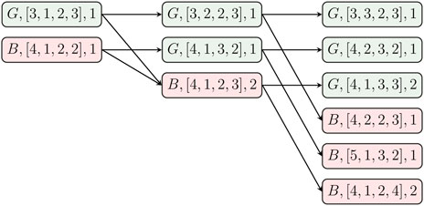
FIGURE 2. An example of how the posterior counts and appearance counts are updated for high power transmission is used for two consecutive steps which increases the number of possible posteriors.
4.2 Learning the Channel Parameters for Scheduling
The presented Bayesian framework enables us to incorporate the uncertainty in the channel parameters in the decision making process. More specifically, prior to transmission at each time k the probability distribution of the channel parameters is updated with respect to the available state and observation history up to k − 1. The estimated parameters are then used to evaluate Eq. 7 to obtain the optimal schedule Eq. 6. Then the sensor adopts this schedule for adjusting the transmission power which yields a new observation at k. Repeating this procedure over time increases the accuracy of the learned channel parameters and thus the readjusted schedule. There are, however, several challenges that need to be addressed for implementing this idea in practice.
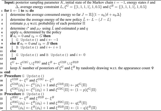
First, as aforementioned, with each high power transmission the number of possible posterior counts grows and thus this number inevitably goes to infinity over time. A common approach to avoid this problem is to ignore the posterior update with high power transmission which leads to a constant number of posterior counts. This approach is not applicable in our problem since it assumes that the underlying two-state Markov chain of the channel remains frozen at those times, as it is in rested bandit problems (Maghsudi and Hossain, 2016). We instead adopt the idea of approximate belief monitoring (Ross et al., 2011; Zou et al., 2016). This method allows us to take into consideration the possible state changes during high power transmissions, while it ensures computational tractability. Essentially, the number of posterior counts kept in the update stage are limited to a constant number K. Moreover, the kept posterior counts are drawn randomly with respect to their appearance count.
The next challenge arises from the dependency of the uncertain channel parameters, optimal schedule and the resulting average energy consumption. The exploration/exploitation dilemma in the presented framework is addressed by applying the schedule in Eq. 6, which is derived based on the average energy constraint. Without explicitly including this constraint in the algorithm, a policy is derived which minimizes the trace of the expected error covariance based on the current posterior distribution of the state and parameters of the channel obtained via the aforementioned Bayesian framework. This tends to leverage the exploration/exploitation toward a better estimation performance at the cost of higher energy consumption and less accurate p and q. To overcome this, we explicitly enforce the energy constrain by utilizing a feedback mechanism in the algorithm as described in Algorithm 1.
We define ξG ≜{[ϕ1, ϕ2, ϕ3, ϕ4], Ψ, Π} as the set of information on the posteriors of the channel being in G and let Π denote the joint probability distribution Eq. 13, which is set to 0.5 initially. Each posterior count in ξG can transition into G or B with probability of 1 − p and p, respectively, where p is the mean of the corresponding Beta distribution (p = ϕ1/(ϕ1 + ϕ2)). Similarly, we define ξB for the posterior counts associated with the channel state B and the corresponding transition probabilities are determined based on their respective q = ϕ3/(ϕ3 + ϕ4). These operations are shown by the two procedures on Line 19 and Line 23. After the update, these sets are merged which is shown by the operator ∪ , such that Ψ and Π of the items with identical posterior counts are summed and then only K posteriors are kept as shown in Line 17 and Line 17, respectively.
To ensure that exploration/exploitation is performed in a manner that the average energy consumption of the returned policy is L, the following corrections are made at each time step k:
• First, the average energy consumed in previous steps is computed in Line 4.
• The average energy constraint for the desired policy is then determined according to Line 4 and it is denoted by
• The values of
This method guarantees that the energy constraint is satisfied regardless of the accuracy of the learned parameters and leads to near-optimal performance as shown in Section 5.
Algorithm 1. Joint learning and scheduling design.
5 Numerical Results
To evaluate the performance of our proposed scheduling methods, we consider a dynamical system with the following parameters
We assume that the parameters of the underlying GE channel connecting the sensor to the remote estimator are p = 0.3 and q = 0.5. With these parameters, it is to calculate the critical recovery rate of the channel as qc = 1–1/1.22 = 0.3 and since q > qc the filter is stable even if the sensor constantly transmits with low power. The following results have been obtained for the scenario in which the high power and low power transmission energies are Δ = 10 and δ = 1, respectively.
First, we consider the case where the energy constraint is given by L = 1.5. Substituting the aforementioned values in Eq. 7 yields
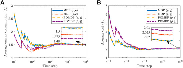
FIGURE 3. Average energy consumption (A), and average trace of error covariance (B), when L = 1.5.
Next, we lift the assumption of known channel parameters, i.e., p and q, and consider two separate scenarios. In the first one, denoted by MDP
An interesting observation is that MDP
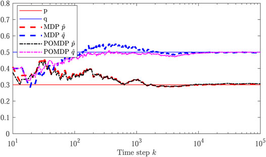
FIGURE 4. Evolution of the learned channel parameters in comparison with the actual values p = 0.3 and q = 0.5.
To investigate the frequency of partial observations, we next consider the energy constraint to be raised to L = 2. A higher energy budget naturally means that the sensor is able to utilize the high power mode more frequently. Consequently, channel state transitions will be observed less frequently thus leading to less accurate estimates of the channel parameters. Using this new constraint we obtain
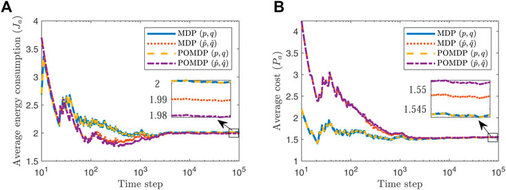
FIGURE 5. Average energy consumption (A), and average trace of error covariance (B), when L = 2.
Next, we consider how violation of the optimality condition Eq. 10 in Lemma 1 affects performance. Recall that for the chosen system parameters Eq. 10 yields 1 ≤ L ≤ 3.25 and thus we let L = 3.35. By assuming that the state of the channel is observable in case of high power transmission, the policy Eq. 6 can be implemented for achieving optimal performance for both known and unknown channel parameters. For the POMDP case, however, we adopt the suboptimal policy proposed in Remark 1. As Figure 6 demonstrates, this results in worse performance in terms of the error covariance compared with the MDP counterpart. Nevertheless, this is expected, as the suboptimal policy of Remark 1 guarantees lower energy consumption than the specified budget while enabling adoption of a deterministic policy. Moreover, as it can be seen from Figures 3, 5, 6, as the energy budget increases, the error covariance at the estimator decreases thus leading to better performance.
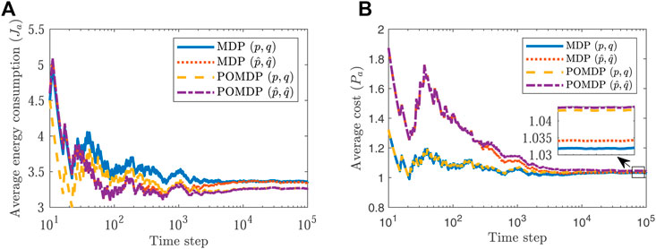
FIGURE 6. Average energy consumption (A), and average trace of error covariance (B), when L = 3.35.
6 Conclusion
We considered the power scheduling of a battery-powered smart sensor with two power modes for remote state estimation over a GE channel. We presented the optimal schedule with full state observation and known channel parameters. When the channel states are only partially observable (only observable with low power transmission), the scheduling problem can be formulated as a POMDP for which we provided the optimal solution and derived the conditions that guarantee its optimality. When in addition to the partially available observations the channel parameters are also unknown, we showed that Bayesian inference can be used to learn these parameters. We then proposed a computationally tractable method to implement this idea in a manner that ensures the energy constraint is met while achieving near-optimal performance.
Data Availability Statement
The raw data supporting the conclusions of this article will be made available by the authors, without undue reservation.
Author Contributions
All authors listed have made a substantial, direct, and intellectual contribution to the work and approved it for publication.
Funding
This work was supported by the Academy of Finland under Grant 13346070. The work of TC was supported by the Academy of Finland under Grant 317726.
Conflict of Interest
The authors declare that the research was conducted in the absence of any commercial or financial relationships that could be construed as a potential conflict of interest.
Publisher’s Note
All claims expressed in this article are solely those of the authors and do not necessarily represent those of their affiliated organizations, or those of the publisher, the editors and the reviewers. Any product that may be evaluated in this article, or claim that may be made by its manufacturer, is not guaranteed or endorsed by the publisher.
References
Alam, F., Mehmood, R., Katib, I., Albogami, N. N., and Albeshri, A. (2017). Data Fusion and IoT for Smart Ubiquitous Environments: A Survey. IEEE Access 5, 9533–9554. doi:10.1109/access.2017.2697839
Chen, L., Hu, B., Guan, Z.-H., Zhao, L., and Zhang, D.-X. (2021). Control-aware Transmission Scheduling for Industrial Network Systems over a Shared Communication Medium. IEEE Internet Things J., 1. doi:10.1109/jiot.2021.3127911
Eisen, M., Rashid, M. M., Gatsis, K., Cavalcanti, D., Himayat, N., and Ribeiro, A. (2019). Control Aware Radio Resource Allocation in Low Latency Wireless Control Systems. IEEE Internet Things J. 6, 7878–7890. doi:10.1109/jiot.2019.2909198
Elliott, E. O. (1963). Estimates of Error Rates for Codes on Burst-Noise Channels. Bell Syst. Tech. J. 42, 1977–1997. doi:10.1002/j.1538-7305.1963.tb00955.x
Farjam, T., Charalambous, T., and Wymeersch, H. (2019). “Timer-based Distributed Channel Access in Networked Control Systems over Known and Unknown Gilbert-Elliott Channels,” in European Control Conference (ECC) (Naples, Italy: IEEE), 2983–2989. doi:10.23919/\1ecc.2019.879617710.23919/ecc.2019.8796177
Farjam, T., Fardno, F., and Charalambous, T. (2020). “Power Allocation of Sensor Transmission for Remote Estimation over an Unknown Gilbert-Elliott Channel,” in European Control Conference (ECC) (Russia: St. Petersburg), 1461–1467. doi:10.23919/ecc51009.2020.9143632
Farjam, T., Wymeersch, H., and Charalambous, T. (2021). Distributed Channel Access for Control over Unknown Memoryless Communication Channels. IEEE Trans. Automat. Contr., 1. doi:10.1109/tac.2021.3129737
Forootani, A., Iervolino, R., Tipaldi, M., and Dey, S. (2022). Transmission Scheduling for Multi-Process Multi-Sensor Remote Estimation via Approximate Dynamic Programming. Automatica 136, 110061. doi:10.1016/j.automatica.2021.110061
Gatsis, K., Ribeiro, A., and Pappas, G. J. (2014). Optimal Power Management in Wireless Control Systems. IEEE Trans. Automat. Contr. 59, 1495–1510. doi:10.1109/tac.2014.2305951
Gilbert, E. N. (1960). Capacity of a Burst-Noise Channel. Bell Syst. Tech. J. 39, 1253–1265. doi:10.1002/j.1538-7305.1960.tb03959.x
Han, D., Wu, J., Zhang, H., and Shi, L. (2017). Optimal Sensor Scheduling for Multiple Linear Dynamical Systems. Automatica 75, 260–270. doi:10.1016/j.automatica.2016.09.015
Kaelbling, L. P., Littman, M. L., and Cassandra, A. R. (1998). Planning and Acting in Partially Observable Stochastic Domains. Artif. Intelligence 101, 99–134. doi:10.1016/s0004-3702(98)00023-x
Knorn, S., Dey, S., Ahlen, A., and Quevedo, D. E. (2019). Optimal Energy Allocation in Multisensor Estimation over Wireless Channels Using Energy Harvesting and Sharing. IEEE Trans. Automat. Contr. 64, 4337–4344. doi:10.1109/tac.2019.2896048
Knorn, S., and Dey, S. (2017). Optimal Energy Allocation for Linear Control with Packet Loss under Energy Harvesting Constraints. Automatica 77, 259–267. doi:10.1016/j.automatica.2016.11.036
Lee, J., Bagheri, B., and Kao, H.-A. (2015). A Cyber-Physical Systems Architecture for Industry 4.0-based Manufacturing Systems. Manufacturing Lett. 3, 18–23. doi:10.1016/j.mfglet.2014.12.001
Leong, A. S., Quevedo, D. E., and Dey, S. (2018). Optimal Control of Energy Resources for State Estimation over Wireless Channels. Springer International Publishing. doi:10.1007/978-3-319-65614-4
Leong, A. S., Ramaswamy, A., Quevedo, D. E., Karl, H., and Shi, L. (2020). Deep Reinforcement Learning for Wireless Sensor Scheduling in Cyber-Physical Systems. Automatica 113, 108759. doi:10.1016/j.automatica.2019.108759
Li, Y., Wu, J., and Chen, T. (2018). Transmit Power Control and Remote State Estimation with Sensor Networks: A Bayesian Inference Approach. Automatica 97, 292–300. doi:10.1016/j.automatica.2018.01.023
Liu, W., Quevedo, D. E., Li, Y., Johansson, K. H., and Vucetic, B. (2021). Remote State Estimation with Smart Sensors over Markov Fading Channels. IEEE Trans. Automatic Control., 1. doi:10.1109/tac.2021.3090741
Maghsudi, S., and Hossain, E. (2016). Multi-armed Bandits with Application to 5G Small Cells. IEEE Wireless Commun. 23, 64–73. doi:10.1109/mwc.2016.7498076
Park, P., Coleri Ergen, S., Fischione, C., Lu, C., and Johansson, K. H. (2018). Wireless Network Design for Control Systems: A Survey. IEEE Commun. Surv. Tutorials 20, 978–1013. doi:10.1109/comst.2017.2780114
Pezzutto, M., Schenato, L., and Dey, S. (2021). Transmission Power Allocation for Remote Estimation with Multi-Packet Reception Capabilities. arXiv:2101.12493 [eess.SY].
Qi, Y., Cheng, P., and Chen, J. (2017). Optimal Sensor Data Scheduling for Remote Estimation over a Time-Varying Channel. IEEE Trans. Automat. Contr. 62, 4611–4617. doi:10.1109/tac.2016.2624139
Quevedo, D. E., Ahlen, A., and Johansson, K. H. (2013). State Estimation over Sensor Networks with Correlated Wireless Fading Channels. IEEE Trans. Automat. Contr. 58, 581–593. doi:10.1109/tac.2012.2212515
Ross, S., Pineau, J., Chaib-draa, B., and Kreitmann, P. (2011). A Bayesian Approach for Learning and Planning in Partially Observable Markov Decision Processes. J. Machine Learn. Res. 12, 1729–1770.
Singh, J., Kaur, R., and Singh, D. (2020). Energy Harvesting in Wireless Sensor Networks: A Taxonomic Survey. Int. J. Energ. Res 45, 118–140. doi:10.1002/er.5816
Wu, J., Jia, Q.-S., Johansson, K. H., and Shi, L. (2013). Event-based Sensor Data Scheduling: Trade-Off between Communication Rate and Estimation Quality. IEEE Trans. Automat. Contr. 58, 1041–1046. doi:10.1109/tac.2012.\1221525310.1109/tac.2012.2215253
Wu, J., Li, Y., Quevedo, D. E., Lau, V., and Shi, L. (2015). Data-driven Power Control for State Estimation: A Bayesian Inference Approach. Automatica 54, 332–339. doi:10.1016/j.automatica.2015.02.019
Wu, J., Shi, G., Anderson, B. D. O., and Johansson, K. H. (2018). Kalman Filtering over Gilbert-Elliott Channels: Stability Conditions and Critical Curve. IEEE Trans. Automat. Contr. 63, 1003–1017. doi:10.1109/tac.2017.2732821
Wu, S., Ren, X., Dey, S., and Shi, L. (2018). Optimal Scheduling of Multiple Sensors over Shared Channels with Packet Transmission Constraint. Automatica 96, 22–31. doi:10.1016/j.automatica.2018.06.019
Xiao, J.-J., Cui, S., Luo, Z.-Q., and Goldsmith, A. J. (2006). Power Scheduling of Universal Decentralized Estimation in Sensor Networks. IEEE Trans. Signal. Process. 54, 413–422. doi:10.1109/tsp.2005.861898
Yang, C., and Shi, L. (2011). Deterministic Sensor Data Scheduling under Limited Communication Resource. IEEE Trans. Signal. Process. 59, 5050–5056. doi:10.1109/tsp.2011.2160863
Zhao, L., Zhang, W., Hu, J., Abate, A., and Tomlin, C. J. (2014). On the Optimal Solutions of the Infinite-Horizon Linear Sensor Scheduling Problem. IEEE Trans. Automat. Contr. 59, 2825–2830. doi:10.1109/tac.2014.2314222
Keywords: power allocation, remote estimation, Gilbert-Elliott channel, partially observable Markov decision process, Bayesian inference
Citation: Farjam T and Charalambous T (2022) Power Allocation for Remote Estimation Over Known and Unknown Gilbert-Elliott Channels. Front. Control. Eng. 3:861055. doi: 10.3389/fcteg.2022.861055
Received: 24 January 2022; Accepted: 15 March 2022;
Published: 14 April 2022.
Edited by:
Yilin Mo, Tsinghua University, ChinaReviewed by:
Alejandro I. Maass, The University of Melbourne, AustraliaLiang Xu, Swiss Federal Institute of Technology Lausanne, Switzerland
Copyright © 2022 Farjam and Charalambous. This is an open-access article distributed under the terms of the Creative Commons Attribution License (CC BY). The use, distribution or reproduction in other forums is permitted, provided the original author(s) and the copyright owner(s) are credited and that the original publication in this journal is cited, in accordance with accepted academic practice. No use, distribution or reproduction is permitted which does not comply with these terms.
*Correspondence: Tahmoores Farjam, tahmoores.farjam@aalto.fi