Effects of the number of simulation iterations and meshing accuracy in monte-carlo random finite-difference analysis

1 Introduction

Geotechnical structures are formed from complex and prolonged physical and chemical processes that are responsible for their inherent uncertainties. Phoon and Kulhawy (1999) identified inherent variability, measurement error, and transformation uncertainty as three principal sources of uncertainty in geotechnical parameters. The consideration of the uncertainty of geotechnical parameters has been a major issue in the numerical simulation of geotechnical structures in recent decades. Currently, random variable (RV) and random field (RF) models are commonly used to simulate geotechnical structures. RV models describe the uncertainty of geotechnical parameters using RVs that follow a certain probability distribution and evaluate the safety of engineering structures based on the reliability index or failure probability. With a well-defined concept and a simple principle, RV models are extensively used to analyze the reliability of geotechnical structures. Chowdhury and Xu (1993) investigated the reliability of homogeneous and layered inhomogeneous slopes using the RV method. However, RV models also have shortcomings: they simply treat geotechnical structures as homogeneous materials and use the reliability index or failure probability to evaluate the safety of engineering structures. Due to factors such as mineral composition and geological activity, the geotechnical parameters at a specific site vary with the location in space. Because RV models neglect the spatial variability of parameters, they method cannot produce accurate analytical results.

Vanmarcke (1977); Vanmarcke (1983) established a relatively sound RF theory that essentially models the characteristic parameters of a soil mass using an RF that follows a homogeneous normal distribution. On this basis, the RF is discretized into RVs. Subsequently, the reliability of the system is determined through the calculation of a large number of RVs and a statistical analysis of the results. This method is referred to as Monte-Carlo random finite-difference analysis (MCRFDA). Numerous researchers (Christian et al., 1994; El-Ramly et al., 2002; Hicks and Samy, 2002; Baecher and Christian, 20062006; Cassidy et al., 2013; Cho, 2014) have employed this method to analyze the reliability of geotechnical engineering structures. Dou and Wang (Dou and Wang, 2017) constructed a one-dimensional non-stationary random field to represent the saturated permeability coefficient of soil, and studied the stability of infinite slope. Cheng et al. (2016) studied the surface deformation of shield tunnel considering the spatial variability of elastic modulus.

As a reliability calculation method originating from engineering practice, Monte Carlo method is both simple and direct but has disadvantages of large amount of calculation. Cho (2007) used Latin hypercube sampling technology to generate random characteristics of soil mass to reduce the calculation amount of Monte Carlo analysis. Ghanem and Spanos (1991) proposed the spectral expansion method of node random variables to reduce the computational effort. The use of MCRFDA first requires the RF to be discretized. The fineness of discretization depends on the size of the generated elements. Computational accuracy increases as the density of elements increases. Refining elements without limit is, however, not possible in actual calculations, which require a balance to be struck between the fineness of the generated elements and computational efficiency. With respect to the number of simulation iterations, N_MC, in MC analysis, a similar balance also needs to be sought between computational accuracy and efficiency. Hence, in this study, we hope to find a balance between these two aims by analyzing a specific model, with the goal of providing a reference for similar problems.

2 Monte-carlo random finite-difference analysis and program realization

The stochastic finite difference method can be divided into two main categories according to the different treatment methods. One is based on analysis to find the relationship between system response and input signal, so as to obtain the law of internal force and deformation of structure and to carry out system reliability analysis. The specific methods include perturbation stochastic finite difference method and Newman stochastic finite difference method. The other is based on statistics, which discretizes the random field into random variables, calculates a large number of random variables and counts the results to obtain the reliability of the system.

The main way to achieve this is Monte-Carlo Random Finite Difference Analysis. Monte Carlo stochastic finite difference method is a theoretical framework for analyzing the influence of spatial variability of geotechnical parameters on geotechnical structures by using stochastic fields. It combines stochastic field theory, finite difference method and Monte-Carlo method. The finite difference method replaces the partial derivative of the function on the grid node with the difference quotient, which is simple and intuitive.

In the Uncertainties Analysis of actual geotechnical engineering, random variables in different spatial locations are described by random field method. This process is the discretization of random field. Vanmarcke (1983) clearly pointed out that random finite element analysis must include the discrete process of random field. There are two main ways to discrete the random field: one is to discrete the random field into random field grid, which is called space discretization; the other is abstract discretization, which expands the random field in series, also called spectral decomposition of random field.

Beacher and Ingra (1981) first proposed stochastic analysis method based on center point method, which Kiureghian and Ke (1988) improved. The center point method uses the random field theory to calculate the random variable value $X\left(u_{io}\right)$ at the centroid of each unit. It considers that the parameters in the unit are constant and equal to the random variable value $X\left(u_{io}\right)$ at the centroid of the unit:

The most criticized point of the center point method is that it assumes that the internal parameters of the cell are completely related, so the calculation accuracy is related to the size of the divided cell. The more closely the cell is divided, the more accurate the calculation result will be. However, when the structure is complex or there are many elements, other discrete methods are difficult to realize. At this time, the advantages of the center point method are particularly prominent.

Based on the studies performed by Cassidy et al. (2013), the covariance matrix decomposition technique is used in this study to generate RFs. The procedure is detailed as follows:

(1) A numerical model of the object of analysis that comprises n elements is established, followed by the extraction of the coordinates of the center of each element.

(2) An autocorrelation function is used to calculate the ρ(x, y, z) of the ith element with respect to all elements (including itself), which yields an nth-order column vector. Subsequently, i is traversed from 1 to n, which produces a matrix, $C_{n\times n}$, comprising n column vectors arranged in i rows. $C_{n\times n}$ is the covariance (autocorrelation) matrix of the model.

(3) The Cholesky decomposition technique is used to decompose $C_{n\times n}$:

where matrix L^T is the transpose of matrix L.

(4) Y is used to denote the resulting n-dimensional column vector. The elements are independent of each other and generally follow a standard normal distribution. We let

where Z is a normally distributed RV with a mean of μ and a variance of $s^2$.

(5) The FISH language is used to assign Z to the corresponding element in the numerical model, generating an MC RF in the Fast Lagrangian Analysis of Continua (FLAC) software. The previous steps are repeated M times to generate all the required MC RFs.

3 Effects of NMC on calculation results

With study Huang et al. (2017) as a reference, a two-dimensional FD model was developed in this study based on a shield subway tunnel in Shanghai. Free, normal displacement-constrained, and fixed boundary conditions were applied to the top (ground surface), sides, and bottom of the model, respectively, as shown in Figure 1.

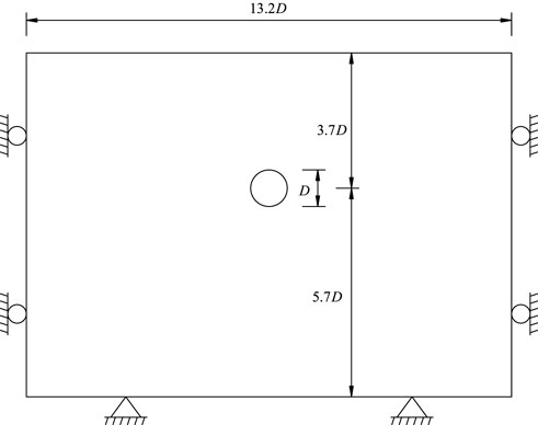
FIGURE 1. Model and boundary diagram.

The FLAC in 3 Dimensions (FLAC3D) numerical analysis software was used to establish a model with 9344 elements, and the tunnel diameter D was set to 6.2 m. To facilitate calculation, the model was set as an elastic constitutive and only considers the condition of complete drying model with a Poisson’s ratio (v) of 0.33 and a density of 1800 kg/m³.

As noted by Fenton and Griffiths (2008), of all soil parameters, elastic modulus E and v are the primary factors affecting soil deformation. Due to its low spatial variability, v is not as important as E in soil deformation analysis. Therefore, only the spatial variability of E generally needs to be considered in the spatial variability analysis of soil deformation. E is assumed to follow a lognormal distribution with a mean of 20 MPa. Variability can be expressed in terms of the coefficient of variation (COV), a dimensionless parameter defined as the ratio of the standard deviation (SD) to the mean. In this study, COV was set to 0.3, and the fluctuation range was set to ${\delta }_x={\delta }_y=2\mathrm{m}$.

A total of 800 RFs of E were generated. Figure 2 shows the spatial distribution of E formed by one typical RF (different element colors represent different E values).

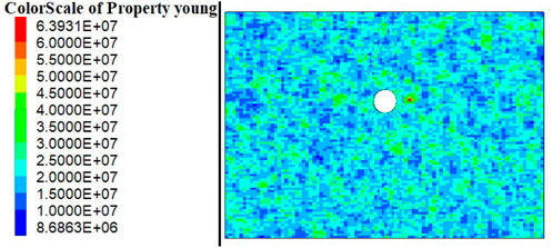
FIGURE 2. Spatial variability distribution of elastic modulus.

The equilibrium state was first calculated under the action of self-weight to generate the original in situ stress field. Subsequently, the horizontal displacement ($D_x$) and vertical displacement ($D_y$) of the contour of the cavern after excavation were calculated, as shown in Figure 3.

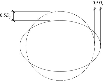
FIGURE 3. Schematic diagram of convergence deformation of cavern.

In MCRFDA, N_MC needs to be determined to produce accurate simulations. Figures 4, 5 show the results for the case examined in this study obtained from calculations based on 800 RFs. After N_MC exceeded 450, the maximum and minimum values of the mean horizontal convergent deformation were 54.34 and 54.18 mm, respectively. This difference of 0.2% suggests that the mean horizontal convergence did not change significantly as N_MC increased beyond 450. After N_MC exceeded 500, the maximum and minimum values of the mean vertical convergent deformation were 207.6 and 207.3 mm, respectively. This difference of 0.1% suggests that the mean vertical convergence did not change significantly as N_MC increased beyond 500. Therefore, for the case examined in this study, calculations based on at least 500 RFs are required to ensure a reasonable mean for convergence.

FIGURE 4. The change of horizontal displacement with the number of simulation groups.

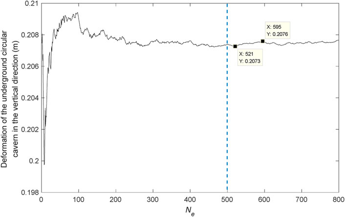
FIGURE 5. The change of vertical displacement with the number of simulation groups.

4 Effects of the fineness of the generated elements on calculation results

The model was divided into different numbers of elements, N_e, while keeping its overall dimension and soil parameters unchanged. For each N_e, calculations were performed based on 500 RFs. Figure 6 shows the distribution of the results.

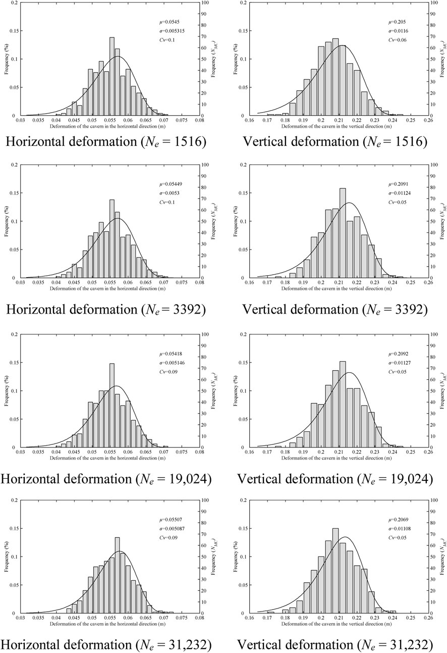
FIGURE 6. Distribution of calculation results using different numbers of elements. Horizontal deformation (N_e = 1516), Vertical deformation (N_e = 1516), Horizontal deformation (N_e = 3392), Vertical deformation (N_e = 3392), Horizontal deformation (N_e = 19,024), Vertical deformation (N_e = 19,024), Horizontal deformation (N_e = 31,232), Vertical deformation (N_e = 31,232).

Figures 7, 8 show the variation in the mean and SD of the convergent deformation of the underground circular cavern with N_e, respectively.

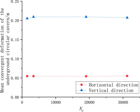
FIGURE 7. Mean value of convergence deformation with different numbers of elements.

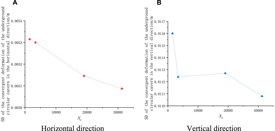
FIGURE 8. Standard deviation of convergence deformation with different numbers of elements. (A) Horizontal direction. (B) Vertical direction.

As shown in Figure 7, the mean of the simulated values did not change significantly as N_e increased. Therefore, it can be concluded that the conventional element size is sufficient to produce high-accuracy simulations using an accurate numerical simulation model.

As shown in Figure 8, in contrast to the mean convergent deformation, the SD of the convergent deformation in each of the horizontal and vertical directions decreased considerably as N_e increased. At a fixed N_e, the simulated values tended to concentrate toward the mean. This finding may suggest that at a fixed spatial variability, increasing the density of elements can increase the uniformity of the distribution of soil parameters, thus reducing the probability of extreme cases.

5 Conclusion

An MCRFDA model of a circular underground cavern is developed. The convergent deformation of the cavern is analyzed with the consideration of the spatial variability of E. The effects of N_MC and N_e on random FD calculations are investigated. The results show the following:

(1) An N_MC greater than 500 is desirable for the random FD analysis of a conventional structure.

(2) For a specific structure, N_e does not have a significant impact on the mean of the simulated values but considerably affects the SD of the simulated values. Reducing N_e increases the SD of the simulated values.

Data availability statement

The raw data supporting the conclusions of this article will be made available by the authors, without undue reservation.

Author contributions

All authors contributed to the study conception and design. Material preparation, data collection and analysis were performed by LC, RB, and PW. The first draft of the manuscript was written by HY and JW, and all authors commented on previous versions of the manuscript. All authors read and approved the final manuscript.

Funding

This research was supported by the key science and technology special program of Yunnan province (No. 202102AF080001).

Conflict of interest

Authors LC, RB, and PW were employed by Yunnan Dianzhong Water Diversion Engineering Co., Ltd.

The remaining authors declare that the research was conducted in the absence of any commercial or financial relationships that could be construed as a potential conflict of interest.

Publisher’s note

All claims expressed in this article are solely those of the authors and do not necessarily represent those of their affiliated organizations, or those of the publisher, the editors and the reviewers. Any product that may be evaluated in this article, or claim that may be made by its manufacturer, is not guaranteed or endorsed by the publisher.

References

Baecher, G. B., and Christian, J. T. (2006, 2006). Geotechnical engineering in the information technology age.The influence of spatial correlation on the performance of Earth structures and foundations, Geo-Congress
Beacher, G. B., and Ingra, T. S. (1981). Stochastic FEM in settlement predictions [J]. J. Geotechnical Eng. Div. 107 (4), 449–463.
Cassidy, M. J., Uzielli, M., and Tian, Y. H. (2013). Probabilistic combined loading failure envelopes of a strip footing on spatially variable soil. Comput. Geotech. 49 (49), 191–205.
Cheng, H. Z., Chen, J., Li, J. B., Hu, Z. F., Li, J. H., and Huang, J. H. (2016). Study on surface deformation induced by shield tunneling based on random field theory. Chin. J. Rock Mech. Eng. (S2), 4256–4264. doi:10.13722/j.cnki.jrme.2016.0099
Cho, S. E. (2007). Effects of spatial variability of soil properties on slope stability[J]. Eng. Geol. 92 (3-4), 97–109.
Cho, S. E. (2014). Probabilistic stability analysis of rainfall-induced landslides considering spatial variability of permeability. Eng. Geol. 171 (8), 11–20.
Chowdhury, R. N., and Xu, D. W. (1993). Rational polynomial technique in lope-reliability analysis. J. Geotech. Eng. 119 (12), 1910–1928.
Christian, J. T., Ladd, C. C., and Baecher, G. B. (1994). Reliability applied to slope stability analysis. ASCE J. Geotech. Eng. 120 (12), 2180–2207.
Dou, H. Q., and Wang, H. (2017). Probabilistic analysis of spatial variability of saturated hydraulic conductivity on infinite slope based on the non-stationary random field. China Civ. Eng. J. (08), 105–113+128. doi:10.15951/j.tmgcxb.2017.08.012
El-Ramly, H., Morgenstern, N. R., and Cruden, D. M. (2002). Probabilistic slope stability analysis for practice. Can. Geotech. J. 39 (3), 665–683.
Fenton, G. A., and Griffiths, D. V. (2008). Risk assessment in geotechnical engineering. Hoboken, New Jersey, USA: John Wiley & Sons.
Ghanem, R. G., and Spanos, P. D. (1991). Spectral stochastic finite-element formulation for reliability analysis[J]. J. Eng. Mech. 117 (10), 2351–2372.
Hicks, M. A., and Samy, K. (2002). Influence of heterogeneity on undrained clay slope stability. Q. J. Eng. Geol. Hydrogeol. 35 (1), 41–49.
Huang, H. W., Xiao, L., Zhang, D. M., and Zhang, J. (2017). Influence of spatial variability of soil Young’s modulus on tunnel convergence in soft soils. Eng. Geol. 228, 357–370.
Kiureghian, A. D., and Ke, J. B. (1988). The stochastic finite element method in structural reliability [J]. Probabilistic Eng. Mech. 3 (2), 83–91.
Phoon, K. K., and Kulhawy, F. H. (1999). Characterization of geotechnical variability. Can. Geotech. J. 36 (4), 612–624.
Vanmarcke, E. H. (1977). Probabilistic modeling of soil profiles. ASCE J. Geotech. Eng. 103 (11), 1227–1246.
Keywords: Monte-Carlo random finite-difference analysis, random field, elastic modulus, cavern deformation, meshing accuracy
Citation: Yu H, Wang J, Cao L, Bai R and Wang P (2023) Effects of the number of simulation iterations and meshing accuracy in monte-carlo random finite-difference analysis. Front. Earth Sci. 10:1041288. doi: 10.3389/feart.2022.1041288
Received: 10 September 2022; Accepted: 20 September 2022;
Published: 06 January 2023.
Edited by:
Junjian Zhang, Shandong University of Science and Technology, ChinaReviewed by:
Lei Xue, Institute of Geology and Geophysics (CAS), ChinaYafeng Zhang, Zhengzhou University of Technology, China
Copyright © 2023 Yu, Wang, Cao, Bai and Wang. This is an open-access article distributed under the terms of the Creative Commons Attribution License (CC BY). The use, distribution or reproduction in other forums is permitted, provided the original author(s) and the copyright owner(s) are credited and that the original publication in this journal is cited, in accordance with accepted academic practice. No use, distribution or reproduction is permitted which does not comply with these terms.
*Correspondence: Rui Bai, 215452297@qq.com