Riverbed Temperature and 4D ERT Monitoring Reveals Heterogenous Horizontal and Vertical Groundwater-Surface Water Exchange Flows Under Dynamic Stage Conditions

Introduction

Groundwater/surface water interactions (GWSW) play a governing role in the biogeochemical function of streams (Woessner, 2000; Boulton et al., 2010; Fleckenstein et al., 2010; Cardenas, 2015; Harvey & Gooseff, 2015). Ecologists have long recognized GWSW exchange as a critical determinant for nutrient cycling, biotic productivity, and microbial function in stream ecosystems (Stanford & Ward, 1988; Boulton, 1993; Storey et al., 1999; Stegen et al., 2018). From a physical perspective, GWSW interaction plays a key role in, for example, buffering stream discharge during runoff events or regulated releases from dams (Woessner, 2000; Arntzen et al., 2006; Cardenas, 2008) and determining patterns of saltwater intrusion into freshwater aquifers (Moore, 1999; Foyle et al., 2002). GWSW interaction also plays a dominant role contaminant fate by influencing physical transport and regulating the biogeochemical reactions facilitated by GW-SW mixing (Ma et al., 2014; Zachara et al., 2016).

Although significant efforts in many disciplines have been expended to understand GWSW interactions and their influences over a range of scales, spatial and temporal patterns of GWSW exchange flows are still not adequately understood (Krause et al., 2014). This is due in large part to the difficulty in observing distributed exchange flow behavior in spatially and temporally heterogeneous systems (Hatch et al., 2006; Kaser et al., 2009; Rosenberry et al., 2013). For example, Briggs & Hare (2018) noted an increasing understanding among the scientific community that groundwater discharge commonly occurs in focused GWSW interaction zones. The common conceptual assumption of spatially diffuse groundwater discharge employed in predictive modeling arises more from the inability to infer focused flows from relatively sparse GWSW measurements than from an unawareness that such flows are prevalent. This highlights the fact that GWSW exchange observations often cannot be collected at the scales required to adequately describe GWSW exchange behavior. In this regard, the advent and use of fiber optic temperature sensing has significantly advanced capabilities to observe distributed GWSW interactions (Selker et al., 2006), but only according to their thermal expressions at the GWSW interface.

Electrical Resistivity Tomography (ERT) has been demonstrated extensively for monitoring GWSW interactions (Cardenas et al., 2010; Slater et al., 2010; Ward et al., 2010; Cardenas & Markowski, 2011; Wallin et al., 2013; Binley et al., 2015; Johnson C. D. et al., 2015; Johnson T. et al., 2015; McLachlan et al., 2017; Parsekian et al., 2015), and has the potential to help fill the spatial information gap between subsurface point sensing and surface expression of GWSW exchange (e.g., fiber optic temperature sensing). Although ERT can help identify the hydrogeologic heterogeneities that govern GWSW exchange (as shown herein), it is most useful when used in time-lapse imaging mode to monitor changes in bulk EC associated with GWRW exchange. For the case presented in this paper, the change in bulk EC arises from the difference in fluid conductivity between groundwater and river water. By subtracting the ERT derived bulk EC image at some background state from the ERT images produced at distinct time intervals, changes in bulk EC associated with GWSW exchange are revealed, thereby indicating when and where the imaging zone is saturated with surface water (less conductive), groundwater (more conductive), or a mixture of the two. The primary advantages of ERT monitoring are its ability to 1) image at customized resolution and scale, 2) be deployed with robust field hardware, 3) autonomously collect data, and 4) remotely detect and image bulk EC changes associated with exchange flows. The primary disadvantages are that 1) the images are resolution limited and are therefore qualitative, 2) bulk EC (or changes therein) are only indirectly informative of hydrogeological, biological, or geochemical processes, 3) ERT is computationally expensive, 4) data processing approaches are not standardized, and 5) accounting for the time-varying water surface boundary in a time-lapse inversion is challenging (Orlando, 2013; McLachlan et al., 2020). Although the advantages of ERT imaging are compelling, the disadvantages have limited its widespread use for GWSW exchange monitoring.

Temperature data have been used extensively to study GWSW interactions (Briggs et al., 2014; Irvine et al., 2017) based on the temperature contrast in groundwater and surface water. In this paper we use a novel combined 3D ERT/thermistor array installed beneath the riverbed to monitor GWSW exchange driven by dynamic stage variations in a high-order managed stream. The objectives of this paper are to:

1) Understand the exchange dynamics of the system and contribute to the overall body of literature describing stage driven GWSW exchange.

2) Demonstrate the flexibility and utility of ERT monitoring for understanding GWSW exchange (e.g., we use pre-existing thermistors as imaging electrodes).

3) Demonstrate an approach for addressing the confounding effects of the moving stage boundary condition, which enables ERT monitoring to be successfully executed.

4) To make progress toward the wider accessibility and use of ERT for GWSW monitoring by providing a “cradle to grave” example of autonomous ERT imaging, including annotated Python scripts and data sets (as Supplementary Video S1) that walk users through the complete analysis using the open source E4D ERT imaging software.

We begin by describing the study area and thermistor array, where the thermistors double as ERT electrodes. We then demonstrate the dominating effects of the river stage boundary on the raw ERT data, and how those effects are removed, enabling successful time-lapse ERT imaging. We then present the time-lapse ERT results and compare them against and with the temperature data time series. Noting that the thermistor array was not designed and not optimal for ERT imaging (rather it was opportunistically used for ERT imaging), the combined ERT and temperature monitoring reveal complex stage driven flow patterns that exhibit high variability over the 10 m by 45 m monitoring zone, including both horizontal and vertical flows. These results suggest that vertical flow assumptions at the GWSW interface should be scrutinized when analyzing GWSW exchange data, particularly under dynamic stage or tidal conditions.

Study Area and Electrical Resistivity Tomography-Thermistor Array

The study area is located on the last free-flowing stretch of the Columbia River, a high-order stream located in south-central Washington (WA) State, United States, approximately 5 km upstream of Richland WA (Figure 1A). River stage variations are governed by outflows from the Priest Rapids Hydroelectric Dam, located approximately 60 km upstream from the study site. Outflows are regulated according to power demands, salmon spawning cycles, and water supply. From 2010 to 2020, volumetric outflows from the dam ranged from approximately 113–11326 m³/s, resulting in stage variations at the study site ranging from approximately 104–110 m in elevation above mean sea level. Stage variations ranged from approximately 104.45–105.29 m over the monitoring period in this study, which lasted from 7 September to 13 September 2018.

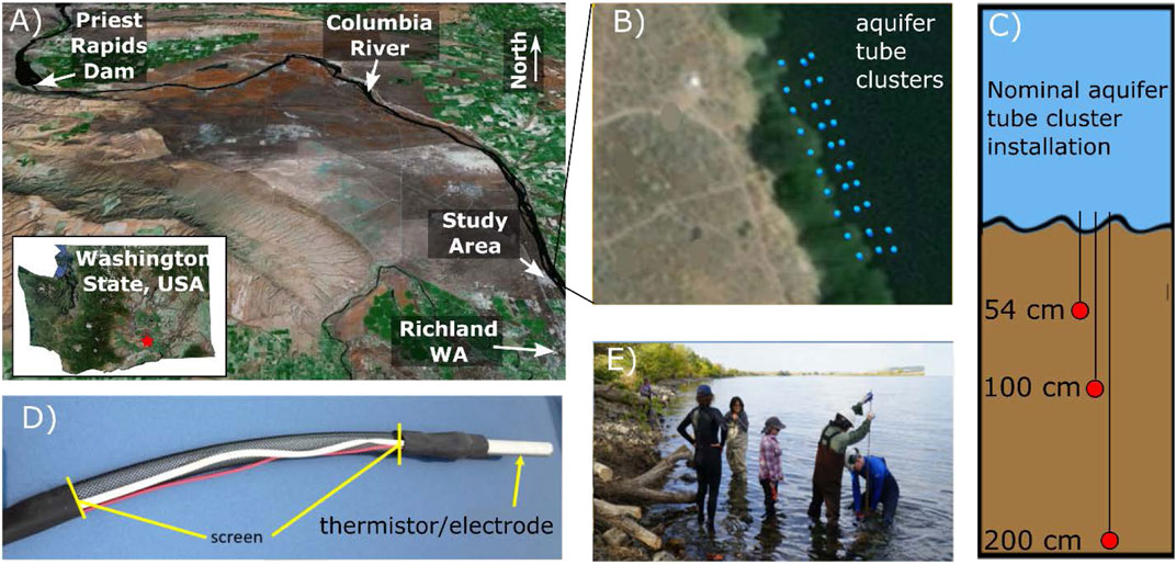
FIGURE 1. (A) Study area location. (B) Plan view map of aquifer tube clusters equipped with depth-discrete thermistor/electrodes. (C) Nominal configuration of an aquifer tube cluster. (D) Photograph of aquifer tube equipped with a thermistor. The thermistor casing is used as an ERT electrode (accessed through the red wire). (E) Photograph of aquifer tube installation.

To study both the physical and biogeochemical responses of the groundwater/surface water interaction zone to stage dynamics, a comprehensive array of 66 aquifer tubes was installed beneath the riverbed near the low-water line (Figures 1B–E). Three 45-m-long transects of 10 piezometer clusters were installed parallel to the shoreline, each transect being.

Separated by approximately 5 m (Figure 1B, Figure 2). Two to three piezometers were installed in close lateral proximity but at different depths in each cluster, ranging from 50 to 200 cm below the riverbed (Figure 1C). To monitor variations in temperature, the tip of each piezometer was instrumented with a metallically housed thermistor. Each thermistor housing was attached to an insulated wire, enabling it to also be used as an ERT electrode (Figure 1D). (Note that testing was conducted to verify that ERT measurements collected using thermistor housings did not interfere with temperature measurements).

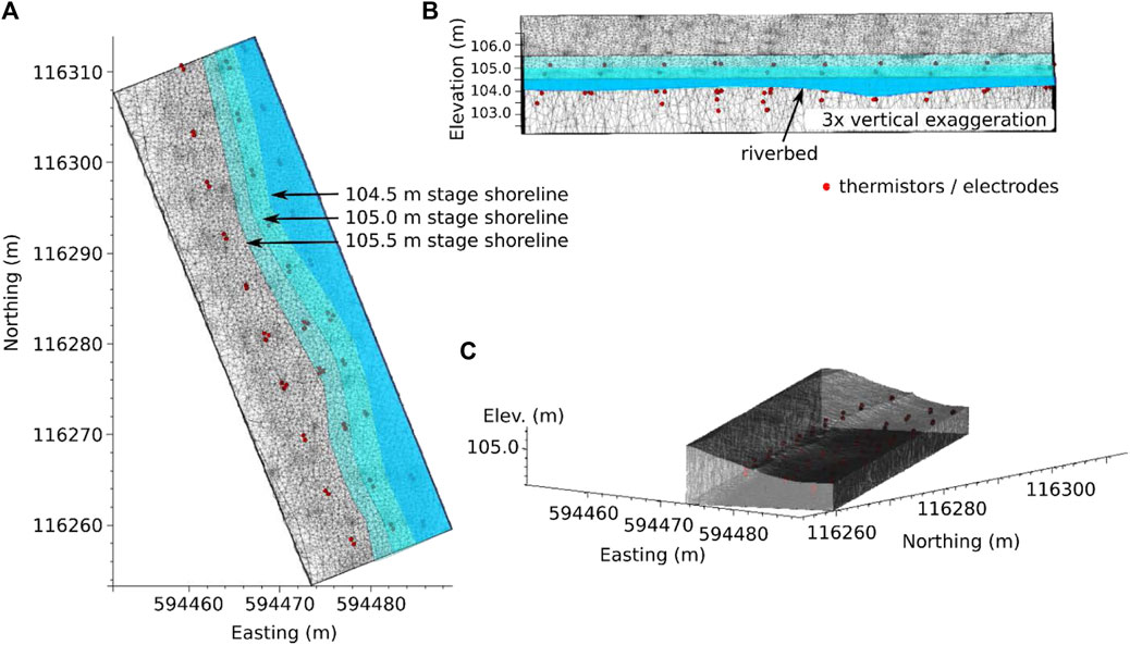
FIGURE 2. (A) Plan view of thermistor/electrode and shoreline locations at three different stage elevations. (B) Cross-section view from river facing westward, showing thermistor/electrode and stage elevations. (C) Oblique view of computational mesh with surface water elements removed to show river bottom bathymetry.

Contrasts between groundwater and river water fluid conductivity enabled time-lapse ERT imaging of groundwater/river water exchange. Over the monitoring period river water temperature and fluid conductivity remained constant at approximately 19.1°C and 0.18 mS/cm, respectively. In contrast, groundwater temperature and fluid conductivity have maintained long-term stability of approximately 14.2°C and 0.42 mS/cm as observed from monitoring wells approximately 50 m inland of the shoreline. The increased fluid conductivity of groundwater causes an increase in bulk electrical conductivity (EC) when pore spaces are filled with groundwater in comparison to river water. This enables river water (or groundwater) to act as a natural contrast agent for time-lapse ERT imaging. For example, Slater et al. (2010), Wallin et al. (2013) and Johnson et al. (2012, Johnson and Wellman, 2015) demonstrated ERT imaging of GWSW interaction, which was enabled by the temperature and fluid conductivity contrasts at the same site.

At the scale of the experiment presented in this paper, the hydrogeology is governed by the younger Hanford formation and the older Ringold Formation. The underlying Ringold Formation is characterized by finer grained lacustrine deposits of relatively low hydraulic conductivity in comparison to the Hanford formation. The Hanford formation is characterized by high-energy sand, gravel and cobble flood deposits with hydraulic conductivities in the range of 1000–5000 m/day (Hammond & Lichtner, 2010). Paleochannels incised into the Ringold Formation by the historical Columbia River have been shown to provide preferred flow paths for groundwater/river water interaction local to the study site (Hammond & Lichtner, 2010). The monitoring array described above was placed to traverse the presumed location of a paleochannel boundary as inferred from previous studies (Slater et al., 2010; Johnson and Wellman, 2015).

Electrical Resistivity Tomography Data and Analysis

Electrical Resistivity Tomography Analysis and Computations

All ERT computations were conducted using the open source E4D software (https://e4d.pnnl.gov). Data and documented Python scripts to reproduce the results presented in this paper are publicly available in the ESS-Dive FAIR standards data repository located at https://ess-dive.lbl.gov/.

Electrical Resistivity Tomography Data

Short, intermediate, and long-offset 3D dipole-dipole ERT data were collected on 66 electrodes using a continuously repeating schedule for the duration of the six-day monitoring period. Measurements were collected using an eight-channel MPT-DAS-1 data collection system (i.e., eight potential measurements per current injection). Each survey required approximately 7 min and consisted of 1013 measurements. After a review of stage levels and ERT data time series, it was determined that hourly subsampling was adequate to capture stage-driven changes in bulk conductivity, so we used one ERT survey per hour for the analysis in this paper.

Correcting for Stage Effects

To illustrate the influence of river stage on the ERT data, a comparison of the river stage and a few ERT data time series is shown in Figure 3. Similar correlations between raw ERT data and stage are common to each ERT measurement time series. Close inspection of stage levels in comparison to riverbed bathymetry (Figure 2) shows that the shoreline migrated directly above the ERT/thermistor array for the duration of the monitoring period. The moving shoreline and variable stage elevation represent a moving zero-flux boundary condition for current flow that significantly influences ERT measurements and must be accounted for in the ERT forward modeling algorithm.

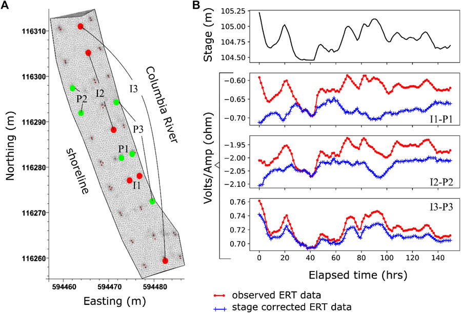
FIGURE 3. (A) Locations of current injection electrodes (I1, I2, and I3) and potential measurement electrodes (P1, P2, and P3) for ERT data time series shown in (B). (B) Stage elevation and ERT observed and stage-corrected measurement time series (i.e., I1-P1 is the voltage observed across electrodes pair P1 given a current of 1 A injection across current pair I1). Each marker indicates an ERT survey time.

Accounting for the moving boundary explicitly requires adaptation of the computational mesh to conform to the stage boundary, which complicates time-lapse imaging (i.e., the computational mesh must be changed at every time-step). Johnson and Wellman, (2015) presented a mesh warping approach to explicitly accommodate moving boundaries (e.g., water table elevations) internal to the mesh. That approach is not applicable in this case because the river bottom boundary must be maintained in a stationary position (i.e., it cannot be moved at the shoreline where the river bottom and top of the river share the same mesh nodes). Instead, we used forward modeling to compute the influence of stage variability on the ERT data with respect to a reference stage position. The time series for each ERT measurement were then corrected to remove stage effects, enabling each time-lapse data set to be inverted on the same mesh (i.e., the mesh for the reference stage position). The steps for the ERT data correction are as follows:

1) Construct a computational mesh with a boundary that conforms to the river bottom bathymetry, and with river mesh elements that conform to the stage and corresponding shoreline at several stage levels (Figures 4A–C).

2) Choose an ERT data set collected when the stage was at one of the levels accommodated by the mesh created in step 1. This is the reference stage level and reference ERT data set.

3) Remove the river water elements that are higher in elevation than the reference stage. The resulting mesh is the reference mesh that will be used to invert the entire ERT time series (Figure 4A).

4) Invert the reference data set on the reference mesh. For this inversion, river water element conductivities were specified at their observed value (0.18 mS/cm) and were not estimated in the inversion. Regularization/smoothing constraints were not applied across the boundary between river water and the subsurface to allow for sharp variations of EC on the inverted mesh at the river bottom boundary. Let the corresponding ERT-estimated EC distribution be referred to as the reference conductivity ${\mathit{\sigma }}_{\mathit{ref}}$ (Figure 4D). Let the ERT data simulated at the reference conductivity be referred to as the reference ERT data ${\mathit{D}}_{\mathit{ref}}$.

5) Map the reference conductivity to the mesh created in step 1. Set the elements representing river water to the observed river water conductivity (Figures 4D–F).

6) Compute the simulated ERT data at each stage elevation $l$ by executing a forward run at each stage on the mesh constructed in step 1 and at the reference conductivity as mapped in step 5. Let the corresponding simulated ERT data be referred to as ${\mathit{D}}_{\mathit{l}}$.

7) Compute stage elevation influence ${\mathit{S}}_{\mathit{l}}$ at stage level $l$ as:

8) Let ${\mathit{D}}_{\mathit{corr},\mathit{t},\mathit{l}}$ be the stage corrected version of the observed ERT data collected at time $t$ and stage $l$, ${\mathit{D}}_{\mathit{obs},\mathit{t},\mathit{l}}$. Then:

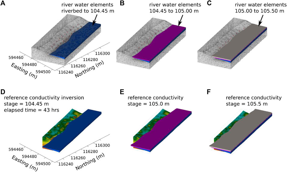
FIGURE 4. Explanation of stage effect computations. (A–C) Computational meshes for three different river stages. Each mesh is identical except for the river water elements. River water elements are added to mesh A to produce mesh B, and to mesh B to produce mesh (C). (D) reference conductivity ${\mathit{\sigma }}_{\mathit{ref}}$ derived by inverting the ERT data ${\mathit{D}}_{\mathit{ref}}\mathit{ }$ collected at 43 h (Figure 2) when the stage was 104.45 m in elevation. (E) Reference conductivity and stage at 105.0 m, used for computing ${\mathit{D}}_{\mathit{l}}$ at $\mathit{l}$ = 105.0 m. (F) Reference conductivity and stage at 105.5 m, used for computing ${\mathit{D}}_{\mathit{l}}$ at $\mathit{l}$ = 105.5 m.

Stage corrections for stage elevations that were not explicitly computed were estimated through linear interpolation of the stage effects at elevations bounding the stage elevation in question. Once ${\mathit{D}}_{\mathit{corr},\mathit{t},\mathit{l}}$ was computed for each time-lapse ERT survey, each data set was inverted on the reference computational mesh to complete the time-lapse imaging. As shown in Figure 4, we chose the reference stage to be 104.45 m, which occurred at an elapsed time of 43 h, and was the lowest stage elevation experienced over the monitoring period. Examples of observed and stage-corrected ERT time series for three representative measurements are shown in Figure 3.

Baseline Electrical Resistivity Tomography Inversion

To investigate changes in groundwater discharge associated with bulk conductivity at the riverbed, we conducted a baseline ERT inversion at time zero when the stage was at its maximum elevation (Figure 3B). Because river water fluid conductivity is less than groundwater fluid conductivity, and river water is driven into the aquifer at high stage, we assumed that the ERT imaging zone was at its lowest conductivity at time zero. As described in the next section, this enables an informative conditional constraint to be placed on the time-lapse inversions, namely that the bulk EC should be greater than or equal to the baseline bulk conductivity at all times and locations.

Reciprocal and repeat ERT measurements collected in close temporal proximity suggested high repeatability and data noise levels that were well below forward simulation accuracy at reasonable mesh sizes. We weighted the ERT data with the error model proposed by Slater et al. (2000):

where $s{d}_i$ is the standard deviation for measurement $i$. $V_i$ and $I_i$ are the potential and current recorded for measurement $i$, respectively. For this work we used $\alpha =0.05$ and $\beta$ = 0.01 ohm, which are consistent with the forward modeling errors shown by Johnson and Wellman, (2015). Using these values, all inversions were fit to a normalized chi-squared value of 1.0.

To regularize the baseline inversion, we used isotropic similarity constraints between neighboring mesh elements. To foster the sharp bulk EC contrast known to exist at the groundwater/surface water interface, regularization constraints were not applied between neighboring river water and river bottom elements. River water element conductivities were set to their known values and were not estimated in the inversion. Theoretical details of the inverse solution and numerical implementation may be found in [Johnson et al., 2012 and Johnson and Wellman, (2015)]. To summarize, the inversion minimizes the objective function:

where ${\mathit{m}}^{\mathit{est}}$ represents the discretized bulk EC distribution, ${\Phi }_d$ is the L-2 norm of the misfit between the observed and simulated ERT data, and ${\Phi }_m$ is a measure of the extent to which ${\mathit{m}}^{\mathit{est}}$ honors the specified regularization constraints. The inversion solution is non-linear, and the inverse algorithm proceeds by iteratively computing linearized updates to ${\mathit{m}}^{\mathit{est}}$ that decrease the value of Eq. 4. The trade-off parameter $\beta$ starts at a large value and is decreased after each inverse update as needed until the target data misfit is achieved (i.e., a normalized chi-squared value of 1.0). The $\beta$ value at convergence was used to determine starting $\beta$ value in the time-lapse inversions as described below.

Time-Lapse Inversions

The time-lapse inversions were weighted and constrained equivalently to the baseline inversion with the following differences:

1) In the time lapse inversion the data sets for each time step are inverted sequentially. The starting model for each time step was the bulk EC solution to the previous time step.

2) The starting $\beta$ value was 1.5 times greater than the value at convergence from the previous time step. $\beta$ was then allowed to decrease as necessary to reach the target chi-squared convergence value. Increasing the starting $\beta$ after at each time step ensures that the final solution is the most homogenous solution that fits the data for the given error model and regularization constraints, or equivalently that ${\Phi }_d$ and ${\Phi }_m$ are optimally minimized.

3) The conductivity is constrained to be greater than or equal the conductivity of the baseline inversion. Such inequality constraints provide significant information to the inversion, resulting in improved resolution (Johnson and Wellman, 2015).

The inequality constraint specified in item 3 above is justified assuming that the bulk conductivity of the subsurface is at its lowest value at baseline (i.e., time zero) when stage elevation is greatest. For all time steps, the inversion converges when the normalized chi-squared value is 1.0. Note that there were no transient regularization constraints specified to smooth bulk conductivity transitions between time steps, or between any time step and the baseline bulk conductivity. Time-lapse ERT results are presented in terms of the change in the base 10 logarithm of bulk conductivity over time, which is computed by subtracting the base 10 logarithm of baseline bulk conductivity from each time step.

Thermistor Data and Analysis

In this paper, we interpret temperature time series in conjunction with time-lapse ERT results to provide a more holistic understanding of dynamic stage-driven exchange flows, and to assist with interpretation and validate of the ERT inversions. Temperature time series at each thermistor location are compared with stage levels to determine the composition of pore water at a given time (i.e., groundwater, river water, or mixed water), based on the observation that that groundwater temperature was14.2°C and river water temperature was 19.1°C over the 150 h monitoring period.

Results

Baseline Electrical Resistivity Tomography

Figure 5 shows observed vs. simulated data fit and a histogram of the weighted residual errors for the baseline inversion. The weighted residual error for measurement $i$ is defined as:

where $d_{i,pred}$ and $d_{i,obs}$ are the simulated and observed resistance values for measurement $i$ and $s{d}_i$ is the corresponding standard deviation defined by Eq. 3. Each time-lapse data set was weighted the same and fit to the same chi-squared value as the baseline data set, so the data fits shown in Figure 5 are representative of the time-lapse inversions also.

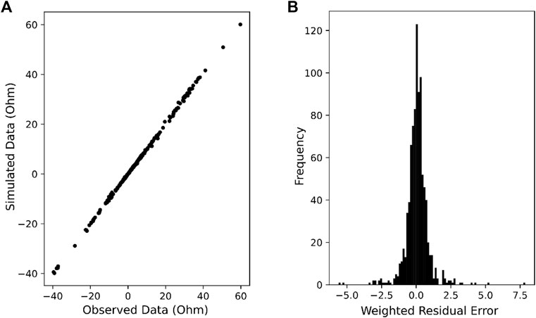
FIGURE 5. Typical data fit statistics for ERT inversions. (A) Simulated vs. observed ERT data at baseline inversion solution. (B) Weighted residual error histogram for baseline inversion.

Figure 6 shows the baseline inversion image. We hypothesize that the massive higher bulk EC zone to the south ranging from 0.01–0.1 S/m is the Ringold Formation, and that the generally lower (<0.01 S/m) bulk EC zone to the north is a paleochannel incised into the Ringold Formation. If that is the case, we expect stage-driven exchange flows to be dominant in the lower bulk EC regions of the baseline image. Figure 6 also shows the sensitivity of the data to the EC distribution from two different views. Sensitivity increases near the electrodes and decreases away from the electrodes. Based on these sensitivities we estimate the depth of investigation to be approximately 100 m in elevation.

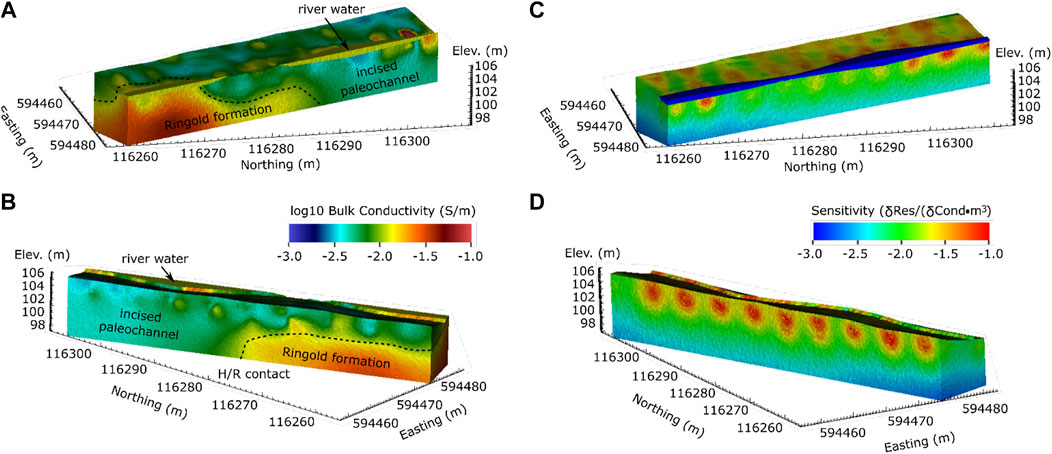
FIGURE 6. (A) View of baseline inversion from river facing westward. (B) View of baseline inversion from shoreline facing northeast. (C) View of data sensitivity to bulk conductivity from river facing westward. (D) View of data sensitivity to bulk conductivity from shoreline facing northeast.

Time-Lapse Electrical Resistivity Tomography and Temperature Comparisons

An animation of the full 4D ERT time-series is provided with the Supplementary Video S1 to this document. Figure 7 shows three different views of the change in bulk EC from high-stage baseline to low stage at 43 h. Regions of increased bulk EC indicate regions where more conductive groundwater has replaced less conductive river water. Time-lapse differences (expressed as 3D isosurfaces) are superimposed on the high bulk EC baseline image anomaly assumed to be the lower permeability Ringold Formation.

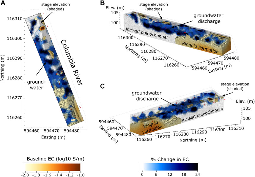
FIGURE 7. (A) Plan view, (B) oblique view from shoreline to river, (C) oblique view from river to shoreline of the change in bulk conductivity from high stage at t = 0 h to low stage at t = 43 h. Changes in bulk EC are represented as semi-transparent isosurfaces, and are diagnostic of where groundwater has replaced river water. Isosurfaces are superimposed on the baseline ERT high-conductivity zone assumed to be the lower permeability Ringold Formation (see Figure 6). Note that Ringold Formation elements do not obfuscate any change in EC isosurfaces (i.e., there are no significant changes within the Ringold Formation). An animation of the full 3D difference time series is included in the supplementary material to this document.

The relative activity of groundwater/river water exchange suggested by the ERT imaging is summarized by the coefficient of variation in Figure 8A, which is the standard deviation normalized by the mean of the bulk EC time series of each mesh element. Regions of elevated coefficient of variation suggest elevated groundwater/river water exchange. Figure 8B shows the stage time series for comparison to Figures 8C,D, which show temperature and bulk EC responses at the six locations indicated in Figure 8A.

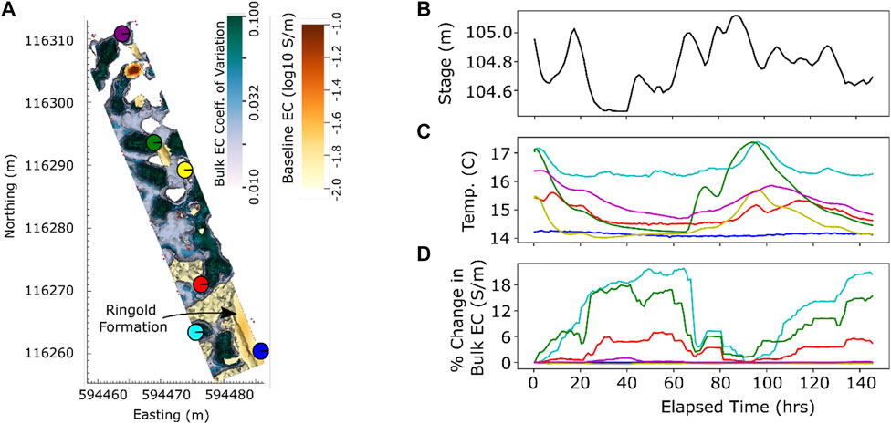
FIGURE 8. (A) Plan view of bulk EC coefficient of variation represented by 3D isosurfaces. Six dots represent colors and locations (∼50 cm beneath the riverbed) of temperature and bulk EC time-series shown in (C) and (D). (B) River stage elevation time series. (C) Temperature time series at the locations shown in (A) River water and groundwater temperatures are respectively 19.1°C and 14.2°C. (D) ERT-derived bulk EC time-series at the locations shown in (A).

Figure 9 shows cross-sections of the bulk EC coefficient of variation along each of the three thermistor/electrode transects parallel to the shoreline. The transect cross-sections suggest that groundwater/river water exchange over the monitoring period is relatively shallow, occurring primarily above approximately 102–103 m in elevation. The L1-L4 cross-section annotations are for convenience in interpreting Figure 10.

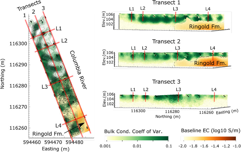
FIGURE 9. Cross sections of bulk EC time-series coefficient of variation along the three thermistor/electrode transects suggest shallow groundwater/surface water interaction. Thermistor responses along lines L1 through L4 are shown in Figure 10.

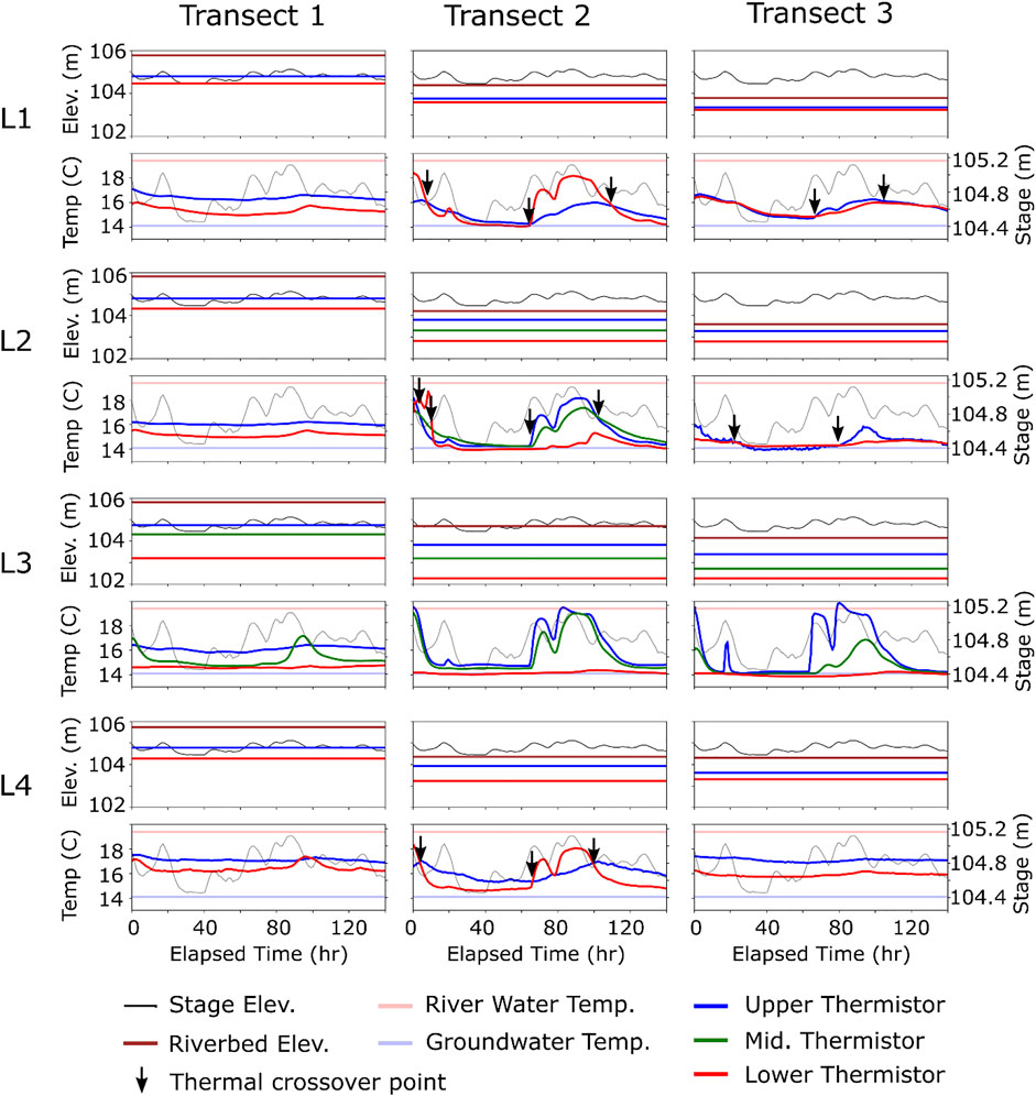
FIGURE 10. Thermistor responses at transect and line intersections shown in Figure 9. For each line (L1–L4) the upper image indicates the elevation of the stage, riverbed, and upper, middle (where present), and lower thermistor. The lower image shows the stage, river water temperature, groundwater temperature, and thermistor temperatures.

Figure 10 shows the thermistor responses at the positions indicated by line (L1-L4) and transect intersections shown in Figure 9. Each position has at least two thermistors installed at different depths below the riverbed (upper and lower), and several positions have a thermistor at intermediate depth. Each plot includes the stage elevation, the elevation of the riverbed, and the elevation of each thermistor at each transect and line intersection. As discussed in the next section, the holistic perspective provided by the combined bulk EC and temperature time series suggest complex patterns of both vertical and horizontal groundwater/river water exchange.

Discussion

Hydrogeologic Interpretation of Baseline Electrical Resistivity Tomography Image

We assumed in the previous section that the high bulk EC region at the southern end of the baseline ERT image was the Ringold Formation, which is known to have relatively low permeability. That assumption is supported by the time-lapse ERT and thermistor data, which show minimal groundwater/river water exchange within the presumed Ringold Formation. In particular, the apparent riverbed outcrop of the Ringold Formation at the southeastern end of the array appears to act as a flow barrier. There is no change in temperature or bulk conductivity in this area for the duration of the monitoring period (Figures 7–10).

Comparison of Temperature and Bulk EC Difference Time Series

Noting that groundwater fluid EC is greater than river water fluid EC (0.42 mS/cm vs. 0.18 mS/cm, respectively) and groundwater temperature is lower than river water temperature (14.2°C vs. 19.1°C, respectively), we may conclude the following from the temperature and bulk EC time series shown in Figure 8:

1) The blue dot is located within the Ringold Formation as presumed from the baseline ERT image. Consistent with this assumption, temperature and bulk EC exhibit no variation with stage, suggesting the blue dot is located within a low-permeability material. Interestingly, the temperature time series suggest this location (and presumably the entire Ringold Formation) is saturated with groundwater for the entire monitoring period.

2) Temperature at the location indicated by the green and light-blue dots suggests these locations are nearly saturated with river water at time zero. Both temperature and bulk EC are highly responsive to stage variations at the green location in comparison to other locations, suggesting a relatively high level of hydrogeologic communication with the river. At the light-blue location, bulk EC is highly responsive to stage but temperature is muted in comparison. This discrepancy may be due in part to the difference in spatial resolution of temperature measurement in comparison to the ERT image.

3) Temperatures at locations indicated by the purple and red dots suggest mixed water at time zero. Both locations exhibit temperature and bulk EC responses to stage, although the bulk EC response at the purple location is muted.

4) Temperature at the location indicated by the yellow dot indicates mixed water at time zero. Stage-driven responses between temperature and bulk EC are inconsistent in this location, which may be attributed differences in resolution.

The temperature time series in Figure 8 demonstrate that (for these locations at least), maximum river water concentrations in the formation occurred at time zero. This supports the assumption that bulk EC was lowest at baseline and justifies the positive change in bulk EC constraint used in the time-lapse inversions. Overall, the spatial and temporal patterns of temperature and bulk EC shown in Figure 8 are qualitatively consistent, especially considering the difference in spatial resolution between the two measurements, and the fact that the ions governing fluid conductivity are likely transported relatively conservatively, and heat is not.

Joint Interpretation of Temperature and Bulk EC Time Series

Bulk EC coefficient of variation cross-sections through transects 1–3 in Figure 9 suggest most of the groundwater/river water exchange activity occurs at elevations above approximately 103 m. These results are consistent with the temperature time series shown in Figure 10. For example, L2 and L3 in Figure 10 are equipped with thermistors near or below 103 m in elevation. In each case, those thermistors maintain groundwater temperature for the entire monitoring period, except for L2 on transect 2 which deviates for short periods during high stage. Both the temperature and bulk EC time series suggest consistent groundwater saturation deeper beneath the riverbed, which implies groundwater discharge deeper into the river and beyond the extent of the current array.

Careful inspection of the ERT image time series suggests a significant component of lateral flow in some parts of the imaging domain (see time-lapse animation in Supplementary Video S1). The temperature time series are also informative in this regard. For example, on L1 transect 2, river water reaches the deeper thermistor before reaching the shallow thermistor during a period of rising stage, which is only possible if there is horizontal transport. Furthermore, the temperature time series between the upper and lower thermistors ‘cross-over’ at three different times during the monitoring period, which to our knowledge is only possible with horizontal transport of thermally stratified water. This same cross-over behavior is also observed in L1 transect 1, L2 transect 2, L2 transect 3, and L4 transect 2 (see black arrows in Figure 10), indicating horizontal flow in each those locations. These results suggest that vertical flow assumptions at the GWSW interface should be scrutinized when analyzing GWSW exchange data, particularly under dynamic stage or tidal conditions.

In contrast, temperature time series in L3 transects 2 and 3 suggest dominant vertical transport. River water reaches the upper thermistor before the lower thermistor during periods of rising stage, and groundwater reaches the lower thermistor before the upper thermistor during periods of falling stage. The vertical temperature profiles also demonstrate characteristics of the groundwater/river water mixing zone. For example, at 85 h on L3 transect 3, the lower thermistor is at groundwater temperature and the upper thermistor is at river water temperature, demonstrating a complete transition from groundwater to river water over a vertical interval of approximately 1.5 m. Both temperature and bulk EC time series indicate a high degree of connectivity to the river along L3 at transects 2 and 3.

Except for L3, the temperatures along transect 1 suggest mixed water and muted responses to river stage. The ERT data suggest most of the exchange activity along transect 1 occurs beneath the elevation of the thermistors (Figure 9, transect 1), and therefore would not be detected.

To further illustrate the heterogeneous nature stage-driven exchange flows, note that L2 transect 3 remains near groundwater temp for the duration of the monitoring period, even though the thermistors are less than 70 cm beneath the riverbed. This is consistent with the muted bulk EC response (e.g., Figure 9, plan view) in the same location. The dominant low-frequency variability of the temperature time-series for both thermistors suggest this location is not well hydrogeologically connect to the river hydrogeologically. In contrast, L3 on transect 3, where the upper two thermistor locations exhibit high connectivity with the river although each is greater than 1.0 m from the riverbed. This difference in exchange activity over 15 m along transect 3 is evident in both the temperature end bulk EC time series, and is exemplary of focused exchange (Briggs & Hare, 2018).

Comments on Electrical Resistivity Tomography Monitoring

We noted previously that the thermistor array was opportunistically used as an ERT array by using the thermistor casings as electrodes. ERT imaging was not considered when designing thermistor spacings, and the array was not optimized for imaging at this scale (i.e., ideally the electrodes would have closer spacing). Regardless, the ERT images revealed complex spatial and temporal stage-driven flow patterns, illustrating the rich information available in the ERT monitoring data concerning GWSW exchange. We would anticipate improved results with an optimized array. Also, rather than using electrodes installed beneath the shallow riverbed, electrodes could be placed on the riverbed surface analyzed in the same method as outlined in this paper, which would significantly simplify deployment. In any case, care should be taken through pre-modelling to other feasibility assessment to ensure sufficient ERT sensitivity to the subsurface under given conditions, particularly in the case of saline surface water.

Summary

We have demonstrated a combined array of thermistors and electrodes for monitoring dynamic, stage-driven groundwater/river water exchanges using point measurements of temperature and 3D time-lapse ERT images of changes in bulk EC. The ERT images were enabled by removing the effects of the moving river stage boundary in the raw ERT data. The combined results reveal complex patterns of dynamic exchange that would be difficult to elicit from either data set alone. For example, the time-lapse ERT images reveal spatial variability in exchange in the horizontal direction (Figure 9), while the thermistor data reveal dynamics in the vertical direction. In contrast to the vertical flow commonly assumed under steady state conditions, the combined analysis suggests significant components of lateral exchange flow under dynamic conditions.

Data Availability Statement

The raw data supporting the conclusions of this article will be made available by the authors, without undue reservation.

Author Contributions

TJ—Data processing and interpretation, writing, figure generation, data curation. JT: ERT system deployment and data collection. CS—Thermistor system design and operation. AG—Field Coordination. JS—Project Management.

Funding

Pacific Northwest National Laboratory is operated by Battelle Memorial Institute for the U.S. Department of Energy under Contract No. DE-AC05-76RL01830. This research was supported by the U.S. Department of Energy (DOE), Office of Biological and Environmental Research (BER), as part of BER’s Subsurface Biogeochemistry Research Program (SBR). This contribution originates from the SBR Scientific Focus Area (SFA) at the Pacific Northwest National Laboratory (PNNL).

Conflict of Interest

The authors declare that the research was conducted in the absence of any commercial or financial relationships that could be construed as a potential conflict of interest.

Publisher’s Note

All claims expressed in this article are solely those of the authors and do not necessarily represent those of their affiliated organizations, or those of the publisher, the editors and the reviewers. Any product that may be evaluated in this article, or claim that may be made by its manufacturer, is not guaranteed or endorsed by the publisher.

Supplementary Material

The Supplementary Material for this article can be found online at: https://www.frontiersin.org/articles/10.3389/feart.2022.910058/full#supplementary-material

References

Arntzen, E. V., Geist, D. R., and Dresel, P. E. (2006). Effects of Fluctuating River Flow on Groundwater/surface Water Mixing in the Hyporheic Zone of a Regulated, Large Cobble Bed River. River Res. applic. 22 (8), 937–946. doi:10.1002/rra.947
Bayani Cardenas, M. (2008). The Effect of River Bend Morphology on Flow and Timescales of Surface Water-Groundwater Exchange across Pointbars. J. Hydrology 362 (1-2), 134–141. doi:10.1016/j.jhydrol.2008.08.018
Binley, A., Hubbard, S. S., Huisman, J. A., Revil, A., Robinson, D. A., Singha, K., et al. (2015). The Emergence of Hydrogeophysics for Improved Understanding of Subsurface Processes over Multiple Scales. Water Resour. Res. 51 (6), 3837–3866. doi:10.1002/2015wr017016
Boulton, A. J., Datry, T., Kasahara, T., Mutz, M., and Stanford, J. A. (2010). Ecology and Management of the Hyporheic Zone: Stream-Groundwater Interactions of Running Waters and Their Floodplains. J. North Am. Benthol. Soc. 29 (1), 26–40. doi:10.1899/08-017.1
Boulton, A. (1993). Stream Ecology and Surface-Hyporheic Hydrologic Exchange: Implications, Techniques and Limitations. Mar. Freshw. Res. 44 (4), 553–564. doi:10.1071/mf9930553
Briggs, M. A., and Hare, D. K. (2018). Explicit Consideration of Preferential Groundwater Discharges as Surface Water Ecosystem Control Points. Hydrol. Process. 32 (15), 2435–2440. doi:10.1002/hyp.13178
Briggs, M. A., Lautz, L. K., Buckley, S. F., and Lane, J. W. (2014). Practical Limitations on the Use of Diurnal Temperature Signals to Quantify Groundwater Upwelling. J. Hydrology 519, 1739–1751. doi:10.1016/j.jhydrol.2014.09.030
Cardenas, M. B. (2015). Hyporheic Zone Hydrologic Science: A Historical Account of its Emergence and a Prospectus. Water Resour. Res. 51 (5), 3601–3616. doi:10.1002/2015wr017028
Cardenas, M. B., and Markowski, M. S. (2011). Geoelectrical Imaging of Hyporheic Exchange and Mixing of River Water and Groundwater in a Large Regulated River. Environ. Sci. Technol. 45 (4), 1407–1411. doi:10.1021/es103438a
Cardenas, M. B., Zamora, P. B., Siringan, F. P., Lapus, M. R., Rodolfo, R. S., Jacinto, G. S., et al. (2010). Linking Regional Sources and Pathways for Submarine Groundwater Discharge at a Reef by Electrical Resistivity Tomography, Rn-222, and Salinity Measurements. Geophys. Res. Lett. 37, Artn L1640110. doi:10.1029/2010gl044066
Fleckenstein, J. H., Krause, S., Hannah, D. M., and Boano, F. (2010). Groundwater-surface Water Interactions: New Methods and Models to Improve Understanding of Processes and Dynamics. Adv. Water Resour. 33 (11), 1291–1295. doi:10.1016/j.advwatres.2010.09.011
Foyle, A., Henry, V., and Alexander, C. (2002). Mapping the Threat of Seawater Intrusion in a Regional Coastal Aquifer-Aquitard System in the Southeastern United States. Environ. Geol. 43 (1-2), 151–159. doi:10.1007/s00254-002-0636-6
Hammond, G. E., and Lichtner, P. C. (2010). Field-scale Model for the Natural Attenuation of Uranium at the Hanford 300 Area Using High-Performance Computing. Water Resour. Res. 46, Artn W09527. doi:10.1029/2009wr008819
Harvey, J., and Gooseff, M. (2015). River Corridor Science: Hydrologic Exchange and Ecological Consequences from Bedforms to Basins. Water Resour. Res. 51 (9), 6893–6922. doi:10.1002/2015wr017617
Hatch, C. E., Fisher, A. T., Revenaugh, J. S., Constantz, J., and Ruehl, C. (2006). Quantifying Surface Water-Groundwater Interactions Using Time Series Analysis of Streambed Thermal Records: Method Development. Water Resour. Res. 42 (10), Artn W10410. doi:10.1029/2005wr004787
Irvine, D. J., Briggs, M. A., Lautz, L. K., Gordon, R. P., McKenzie, J. M., and Cartwright, I. (2017). Using Diurnal Temperature Signals to Infer Vertical Groundwater‐Surface Water Exchange. Groundwater 55 (1), 10–26. doi:10.1111/gwat.12459
Johnson, C. D., Swarzenski, P. W., Richardson, C. M., Smith, C. G., Kroeger, K. D., and Ganguli, P. M. (2015). Ground-truthing Electrical Resistivity Methods in Support of Submarine Groundwater Discharge Studies: Examples from Hawaii, Washington, and California. Jeeg 20 (1), 81–87. doi:10.2113/Jeeg20.1.81
Johnson, T. C., Slater, L. D., Ntarlagiannis, D., Day-Lewis, F. D., and Elwaseif, M. (2012). Monitoring Groundwater-Surface Water Interaction Using Time-Series and Time-Frequency Analysis of Transient Three-Dimensional Electrical Resistivity Changes. Water Resour. Res. 48, Artn W07506. doi:10.1029/2012wr011893
Johnson, T. C., and Wellman, D. (2015). Accurate Modelling and Inversion of Electrical Resistivity Data in the Presence of Metallic Infrastructure with Known Location and Dimension. Geophys. J. Int. 202 (2), 1096–1108. doi:10.1093/gji/ggv206
Johnson, T., Versteeg, R., Thomle, J., Hammond, G., Chen, X., and Zachara, J. (2015). Four-dimensional Electrical Conductivity Monitoring of Stage-Driven River Water Intrusion: Accounting for Water Table Effects Using a Transient Mesh Boundary and Conditional Inversion Constraints. Water Resour. Res. 51 (8), 6177–6196. doi:10.1002/2014wr016129
Käser, D. H., Binley, A., Heathwaite, A. L., and Krause, S. (2009). Spatio-temporal Variations of Hyporheic Flow in a Riffle-Step-Pool Sequence. Hydrol. Process. 23 (15), 2138–2149. doi:10.1002/hyp.7317
Krause, S., Boano, F., Cuthbert, M. O., Fleckenstein, J. H., and Lewandowski, J. (2014). Understanding Process Dynamics at Aquifer-Surface Water Interfaces: An Introduction to the Special Section on New Modeling Approaches and Novel Experimental Technologies. Water Resour. Res. 50 (2), 1847–1855. doi:10.1002/2013wr014755
Ma, R., Liu, C., Greskowiak, J., Prommer, H., Zachara, J., and Zheng, C. (2014). Influence of Calcite on Uranium(VI) Reactive Transport in the Groundwater-River Mixing Zone. J. Contam. Hydrology 156, 27–37. doi:10.1016/j.jconhyd.2013.10.002
McLachlan, P., Chambers, J., Uhlemann, S., Sorensen, J., and Binley, A. (2020). Electrical Resistivity Monitoring of River-Groundwater Interactions in a Chalk River and Neighbouring Riparian Zone. Near Surf. Geophys. 18 (4), 385–398. doi:10.1002/nsg.12114
McLachlan, P. J., Chambers, J. E., Uhlemann, S. S., and Binley, A. (2017). Geophysical Characterisation of the Groundwater-Surface Water Interface. Adv. Water Resour. 109, 302–319. doi:10.1016/j.advwatres.2017.09.016
Moore, W. S. (1999). The Subterranean Estuary: a Reaction Zone of Ground Water and Sea Water. Mar. Chem., 65(1-2), 111–125. doi:10.1016/S0304-4203(99)00014-6
Orlando, L. (2013). Some Considerations on Electrical Resistivity Imaging for Characterization of Waterbed Sediments. J. Appl. Geophys. 95, 77–89. doi:10.1016/j.jappgeo.2013.05.005
Parsekian, A. D., Singha, K., Minsley, B. J., Holbrook, W. S., and Slater, L. (2015). Multiscale Geophysical Imaging of the Critical Zone. Rev. Geophys. 53 (1), 1–26. doi:10.1002/2014rg000465
Rosenberry, D. O., Sheibley, R. W., Cox, S. E., Simonds, F. W., and Naftz, D. L. (2013). Temporal Variability of Exchange between Groundwater and Surface Water Based on High-Frequency Direct Measurements of Seepage at the Sediment-Water Interface. Water Resour. Res., 49(5), 2975–2986. doi:10.1002/wrcr.20198
Selker, J., van de Giesen, N., Westhoff, M., Luxemburg, W., and Parlange, M. B. (2006). Fiber Optics Opens Window on Stream Dynamics. Geophys. Res. Lett. 33 (24), Artn L24401. doi:10.1029/2006gl027979
Slater, L., Binley, A. M., Daily, W., and Johnson, R. (2000). Cross-hole Electrical Imaging of a Controlled Saline Tracer Injection. J. Appl. Geophys., 44(2-3), 85–102. doi:10.1016/S0926-9851(00)00002-1
Slater, L. D., Ntarlagiannis, D., Day-Lewis, F. D., Mwakanyamale, K., Versteeg, R. J., Ward, A., et al. (2010). Use of Electrical Imaging and Distributed Temperature Sensing Methods to Characterize Surface Water-Groundwater Exchange Regulating Uranium Transport at the Hanford 300 Area, 46. Washington: Water Resources Research, Artn W10533. doi:10.1029/2010wr009110
Stanford, J. A., and Ward, J. V. (1988). The Hyporheic Habitat of River Ecosystems. Nature, 335(6185), 64–66. doi:10.1038/335064a0
Stegen, J. C., Johnson, T., Fredrickson, J. K., Wilkins, M. J., Konopka, A. E., Nelson, W. C., et al. (20182018). Influences of Organic Carbon Speciation on Hyporheic Corridor Biogeochemistry and Microbial Ecology. Nat. Commun. 9, 585ARTN 1034. doi:10.1038/s41467-018-02922-9
Storey, R. G., Fulthorpe, R. R., and Williams, D. D. (1999). Perspectives and Predictions on the Microbial Ecology of the Hyporheic Zone. Freshw. Biol., 41(1), 119–130. doi:10.1046/j.1365-2427.1999.00377.x
Wallin, E. L., Johnson, T. C., Greenwood, W. J., and Zachara, J. M. (2013). Imaging High Stage River-Water Intrusion into a Contaminated Aquifer along a Major River Corridor Using 2-D Time-Lapse Surface Electrical Resistivity Tomography. Water Resour. Res. 49 (3), 1693–1708. doi:10.1002/wrcr.20119
Ward, A. S., Gooseff, M. N., and Singha, K. (2010). Imaging Hyporheic Zone Solute Transport Using Electrical Resistivity. Hydrol. Process., 24(7), 948–953. doi:10.1002/Hyp.7672
Woessner, W. W. (2000). Stream and Fluvial Plain Ground Water Interactions: Rescaling Hydrogeologic Thought. Ground Water, 38(3), 423–429. doi:10.1111/j.1745-6584.2000.tb00228.x
Keywords: groundwater, surface water, hyporheic, resistivity, tomography, monitoring, temperature
Citation: Johnson T, Thomle J, Stickland C, Goldman A and Stegen J (2022) Riverbed Temperature and 4D ERT Monitoring Reveals Heterogenous Horizontal and Vertical Groundwater-Surface Water Exchange Flows Under Dynamic Stage Conditions. Front. Earth Sci. 10:910058. doi: 10.3389/feart.2022.910058
Received: 31 March 2022; Accepted: 16 May 2022;
Published: 06 June 2022.
Edited by:
Sebastian Uhlemann, Berkeley Lab (DOE), United StatesReviewed by:
Adrien Dimech, Université du Québec en Abitibi Témiscamingue, CanadaPaul McLachlan, Aarhus University, Denmark
Copyright © 2022 Johnson, Thomle, Stickland, Goldman and Stegen. This is an open-access article distributed under the terms of the Creative Commons Attribution License (CC BY). The use, distribution or reproduction in other forums is permitted, provided the original author(s) and the copyright owner(s) are credited and that the original publication in this journal is cited, in accordance with accepted academic practice. No use, distribution or reproduction is permitted which does not comply with these terms.
*Correspondence: Tim Johnson, tj@pnnl.gov