Improved Volume-Of-Solid Formulations for Micro-Continuum Simulation of Mineral Dissolution at the Pore-Scale

1 Introduction

Prediction of solid mineral dissolution during reactive flow in porous media is vital for a wide range of subsurface applications, including CO₂ sequestration (Black et al., 2015), geothermal systems (Pandey et al., 2015) and enhanced oil recovery (Shafiq and Ben Mahmud, 2017). CO₂ storage in underground reservoirs has the potential to significantly mitigate the environmental impact of many industrial processes. However, mineral dissolution is a potential barrier to the long-term storage of CO₂ in the subsurface, as CO₂ reacts with water to make carbonic acid that can dissolve solid minerals and threaten the structural integrity of a reservoir (Nordbotten and Celia, 2011). In addition, most subsurface applications involve the injection of fluids with chemical properties that are incompatible with existing reservoir fluids and can lead to mineral precipitation or scaling in the pore structure. Scaling is especially prevalent near well-bores, and can significantly reduce the permeability, and thus productivity of a porous formation. Acid injection is then often used to improve the flow in clogged wells (Williams et al., 1979). Thus, accurate and efficient modelling of mineral dissolution in porous media is crucial to improve and optimise these engineering processes.

Modelling reactive transport at the field-scale relies on the assumption that a representative elementary volume can be defined such that flow, transport and reaction can be described in terms of bulk properties like porosity, permeability and macro-scale reactive constant, in what is usually referred as the Darcy scale (Lichtner, 1988; Shapiro and Brenner, 1988; Quintard and Whitaker, 1994; Steefel et al., 2015). Mineral dissolution modifies the pore structure and results in a change in these Darcy-scale properties. Pore-scale numerical experiments can be used to predict the change in these Darcy-scale properties during dissolution. At the pore-scale, these reactions are applied directly on the solid surface while resolving flow and transport in a representative elementary volume of pore space directly. The effects of these dissolution-induced structural changes on the flow and transport properties of the bulk medium can then be estimated for use in Darcy-scale simulations.

The last decade has seen an explosion in the study of flow and transport behaviour at the pore-scale (Noiriel et al., 2009; Raoof et al., 2013; Varloteaux et al., 2013; Starchenko et al., 2016; Menke et al., 2017; Molins et al., 2017; Soulaine et al., 2017; Yang et al., 2020). Recent advances in X-ray imaging techniques have enabled direct observation and quantification of dissolution-induced changes in pore structures (Noiriel et al., 2009; Hao et al., 2013; Luquot et al., 2014; Menke et al., 2015, 2016, 2017, 2018). Numerical modeling has played an important role in these investigation of pore-scale physics, as it provides a mechanistic understanding of the relevant coupled processes. Furthermore, simulation results resolve variables that are not easily available from experiments such as concentration gradients within the pore space.

Numerical modelling of mineral dissolution at the pore-scale can be performed using Pore-Network Modelling (Nogues et al., 2013; Raoof et al., 2013; Varloteaux et al., 2013). However, the evolution of the pore-space can only be predicted using the finite range of geometrical parameters of the network. Alternatively, computational microfluidics (Soulaine et al., 2021a) has been applied using a range of numerical methods (Molins et al., 2020). Interface tracking models explicitly deform and move the solid surface, either using solid balance with a threshold on a lattice (Kang et al., 2002; Szymczak and Ladd, 2009; Prasianakis and Ansumali, 2011), a conforming mesh based on the Arbitrary-Lagrangian-Eulerian (ALE) framework (Starchenko et al., 2016; Starchenko and Ladd, 2018) or smoothed particle hydrodynamics (Tartakovsky et al., 2007). Alternatively, the interface can be captured using a level-set function (Li et al., 2010; Molins et al., 2017). For all these methods, the boundary conditions on the solid surface can be applied directly, or using an immersed boundary condition. However, they require additional treatment for interface displacement, topological changes or remeshing, which usually lead to an increase in their computational cost (Yang et al., 2021).

The micro-continuum approach (Chatelin, Robin et al., 2016; Soulaine and Tchelepi, 2016; Soulaine et al., 2017, 2019; Yang et al., 2021) based on the Volume-of-Solid (VoS) method offers an attractive substitute for interface tracking models. Within this approach, the fluid-solid interface is captured using an indicator function equal to the volume fraction of void space in each cell, and flow and transport are solved using the Darcy-Brinkman-Stokes (DBS) equation. The VoS method is computationally efficient as it does not require remeshing or any special treatment for topological changes.

In the standard VoS approach, the surface area of the fluid-solid interface in a control volume is computed through the gradient of a volume fraction. In practice, a diffuse interface may emerge that spreads across a large number of layers in the computational grid. To enforce the localization of the reactive boundary condition at the fluid/solid interface, a diffuse interface localization function ψ is generally introduced (Soulaine et al., 2017) and this formulation is labelled VoS-ψ. The main advantage of the VoS-ψ method is that standard Reactive Transport Modelling dedicated to Darcy-scale can be easily applied to simulate geochemical processes at the pore-scale by simply changing the way the fluid-rock interfacial area within control volume is estimated (Soulaine et al., 2021b). While the surface area for Darcy-scale simulations is an input parameter that is either constant or depends on complex function of porosity and flow rates (Noiriel et al., 2009; Wen and Li, 2017), the surface area for pore-scale simulations using VoS is directly calculated from the mapping of the solid volume fraction. The main limitation of the VoS − ψ is that the accuracy of the model depends strongly on the choice of the localization function (Luo et al., 2012), and the optimal choice depends on a large number of parameters, such as the geometry, the flow rate, the reactive constant, the computational mesh and the discretization method used for the computation of gradients.

In this paper we propose two novel VoS formulations. The first formulation (iVoS) removes the need for a localization function by computing the reaction rate using the divergence of flux. The second formulation (VoS-ψ’) uses a localization function with a parameter that is fitted to ensure that the reactive surface area is conserved globally. The numerical models are presented in Section 2. The iVoS and VoS-ψ′ methods are then compared with the VoS-ψ method and with an interface tracking method based on the ALE framework on three benchmark test cases in Section 3. In each case, we show that our new VoS methods match accurately experimental results and/or simulation results using the ALE method while being significantly faster.

2 Mathematical Models

In this section, the governing equations and the micro-continuum approach are first presented. Then, we describe the iVoS, VoS-ψ and VoS-ψ’ models, which differ only in the way the reaction rate is computed. Further, we show how dimensionless analysis lead to the quasi-static assumption that reduces the computational time.

2.1 Governing Equations

The governing equations consider flow, transport and reaction at the fluid-solid interface. The domain Ω is partitioned into fluid Ω_f and solid Ω_s. Under isothermal conditions and in the absence of gravitational effects, fluid motion in Ω_f is governed by the incompressible Navier-Stokes equations

with the continuity condition at the fluid-solid interface Γ,

where u (m/s) is the velocity, p (m²/s²) is the kinematic pressure, ν (m²/s) is the kinematic viscosity, ρ (kg/m³) is the fluid density, ρ_s (kg/m³) is the solid density, n_s is the normal vector to the fluid-solid interface pointing toward the solid phase, and w_s (m/s) is the velocity of the fluid-solid interface, which is controlled by the surface reaction rate R (kmol/m²/s) such that

where M_ws is the molecular weight of the solid. The concentration c (kmol/m³) of a species in the system satisfies an advection-diffusion equation

where D (m²/s) is the diffusion coefficient. The chemical reaction occurs at the fluid-solid interface Γ, such that

where ζ is the stoichiometric coefficient of the species in the reaction. In this work, we assume that the surface reaction rate depends only on the concentration of one reactant species, following

where k_c (m/s) is the reaction constant.

2.2 Micro-Continuum Approach With Volume-Of-Solid

In the micro-continuum approach, the entire domain Ω is considered, i. e fluid Ω_f and solid Ω_s, and the fluid-solid interface is tracked in terms of V_f and V_s, the volume of fluid and solid phase in each control volume V, and their volume fraction ɛ = V_f/V and ɛ_s = 1 − ɛ. The flow, transport and chemical reaction are solved in term of the volume-averaged velocity

and the phase-averaged pressure and reactant concentration.

The averaging process results in an extension of the Darcy-Brinkman-Stokes equation (Soulaine et al., 2017)

where k (m²) is the permeability of the cell. $\nu k^{-1}\bar{\mathbf{u}}$ represents the momentum exchange between the fluid and the solid phase, i.e., the Darcy resistance. This term is dominant in the solid phase and vanishes in the fluid phase. To model this, the local permeability field k is assumed to be a function of the local porosity ɛ, following a Kozeny-Carman relationship

where k₀ (m²) is the Kozeny-Carman constant. For the acid transport, the mass-balance equation averaged over the control volume gives

where ɛD* (m²/s) is the effective diffusion coefficient and $\bar{R}$ (kmol/m³/s) is the volume-averaged surface reaction rate. The effective diffusion coefficient takes into account the reduction of the total diffusion due to the presence of solid phase. In this paper, we take D∗ = D. The volume-averaged surface reaction rate is defined as

where A = V ∩Γ is the reactive surface area in the control volume. The specific surface area a_s (m⁻¹) in a control volume is defined as

During the dissolution process, the pore-space evolves with the chemical reaction at the pore surfaces. The number of moles of solid consummed by the chemical reaction is equal to the number of moles of reactant consummed. Therefore, the mass balance equation for the solid phase writes

and the volume averaged velocity satisfies

2.3 Improved Volume-Of-Solid

The method presented here is analogue to the calculation of the mass transfer across a multiphase interface presented in Maes and Soulaine (2020), for which the mass transfer is calculated as the scalar product between a diffusive flux and the gradient of the phase indicator function. To calculate the volume-averaged surface reaction rate, the improved Volume-of-Solid (iVoS) therefore introduces the reactive flux, Φ_R (kmol/m²/s), defined as

and the volume-averaged surface reaction rate can be rewritten as

Assuming that the concentration of the reactant on the reactive surface can be approximated by its volume-averaged on the control volume, and that the normal vector to the interface can be approximated by

the reactive flux can be approximated by

Moreover, the average surface normal in a control volume can be calculated as (Quintard and Whitaker, 1994)

Therefore, the volume-averaged surface reaction rate can be calculated as

To avoid problems related to the calculation of the gradient of ɛ (see Section 2.4), the divergence theorem is used to recast $\bar{R}$ as

With this formulation, the reactive rate is the sum of two terms, an overall mass transfer term $(\sum {\bar{R}}_f=\sum \left(\epsilon \nabla \cdot {\bar{\mathbf{\Phi }}}_R\right))$ and a conservative term $(-\sum \left(\nabla \cdot \left(\epsilon {\bar{\mathbf{\Phi }}}_R\right)\right)=0)$, which balances the local reaction rate between two adjacent control volumes. This means that the reaction can consume reactant in 1 cell and use it to dissolve solid in a neighbor cell. By using a second-order high resolution difference scheme (van Leer, 1974), the reaction rate is balanced toward the reactive surface and the diffusion of the solid interface is limited. This is an accurate representation of a reaction at an interface between 2 cells with ɛ ≈ 0 and ɛ = 1, where the reaction rate is calculated using the concentration in the fluid where ɛ = 1 and the reaction dissolves the solid where ɛ ≈ 0. This formulation is labelled iVoS.

2.4 Volume-Of-Solid With Localization Function

As an alternative to Eq. 24, the volume-averaged surface reaction rate can be calculated as

The specific surface area can be directly calculated as = ‖∇ɛ‖. However, this can lead to a diffuse interface that spreads across a large number of layers in the computational grid. To enforce localization of the dissolution front on the fluid-solid interface, the VoS-psi method introduces a diffuse interface localization function ψ (Soulaine et al., 2017) so that

The main advantage of VoS-ψ compared to iVoS is that it provides a direct calculation of the reactive surface area in a control volume. Therefore, the reaction rate can be calculated by a dedicated geochemical solver, such as Phreeqc (Parkhurst and Wissmeier, 2015) or Reaktoro (Walsh et al.), as it is often done for standard Reactive Transport Modelling dedicated to multi-scale applications (Soulaine et al., 2021b).

While the VoS-ψ method has proved to be a fast and flexible method to match experimental results (Molins et al., 2020), this formulation has one main limitation. It is strongly dependent on the choice of the localization function ψ. Several functions have been proposed by Luo et al. (2012), but their accuracy depends on the case considered and on the discretization scheme used for the gradient. For example, using a centered difference scheme requires ψ(1.0) = 0 for stability. However, using a decentered scheme (in the direction of ɛ = 0 to avoid instabilities) will result in a higher and more diffuse reaction rate, due to a higher reactant concentration away from the surface and a larger specific surface area when ɛ = 0. Centered difference schemes are less diffuse, but they result in incomplete dissolution, since a cell with ɛ < 1 but ɛ = 1 for all its neighbors will have a zero reaction rate. Currently, there is no consensus on the ideal combination of localization function and discretization scheme to use for every scenario, as this will depend on the geometry and flow conditions.

In this work, we use a centered difference scheme for the gradient and ψ = λɛ(1 − ɛ), which is the most accurate combination of discretization scheme and localization function proposed by Luo et al. (2012) for the case of dissolution of a calcite post by acid injection (Soulaine et al., 2017). Typically, λ = 4, but since ψ ≤ 1.0, this will lead to a reduction in interfacial area. For this reason, the VoS-ψ method gives an overall lower dissolution rate that the iVoS method. Instead, λ can be calculated as

In Equ. (27), λ_ɛ is a parameter that depends on the porosity field ɛ in the whole domain and chosen so that the surface area is conserved globally, i. e

In this work, we label VoS-ψ the formulation using $\psi =4\epsilon \left(1-\epsilon \right)$ and VoS-ψ′ the formulation using $\psi ={\lambda }_{\epsilon }\epsilon \left(1-\epsilon \right)$. Using the VoS-ψ′ formulation, the total surface area is conserved globally. However, it is not conserved locally. At an interface between 2 cells with ɛ ≈ 0 and ɛ = 1, the interface area will remain close to 0 in both cells even after the correction.

2.5 Upscaling to the Darcy Scale

In order to investigate the capabilities of our numerical model to calculate upscaled properties for macro-scale simulations, the flow and reaction in the whole domain are characterised by the total porosity ϕ, the Darcy velocity U_D (m/s),

and the permeability K (m²),

where Q_i (m³/s) is the inlet flow rate, A_i (m²) is the inlet area, L_D (m) is the distance between the inlet and outlet, ΔP (m²/s²) is the kinematic pressure drop. In addition, the chemical reaction is characterised by the total specific surface area a (m⁻¹)

and the correction factor α, that represents the reduction of the reactive surface area accessible to reactant, and is defined as

Change in effective upscaling parameters K, a and α are often modelled as a function of porosity with power law functions (Noiriel et al., 2009; Wen and Li, 2017; Seigneur et al., 2019). The parameters of these power-law functions depend strongly on the flow, transport and reaction conditions, which are characterized by the Péclet number

which quantifies the relative importance of advective and diffusive transport, and the Damköhler number

which quantifies the relative importance of chemical reaction and advective transport. Here U and L are the reference velocity and length. The product of the Damköhler and Péclet numbers is also a relevant quantity called the Kinetic number, defined as

In addition, the reactant strength is characterized by

where c_i is the concentration of reactant at the inlet.

3 Benchmark Cases

In this section, the numerical models are benchmarked based on experimental results and simulation results using an interface tracking method based on the ALE framework. All numerical methods are implemented in GeoChemFoam, our reactive transport toolbox, and their implementation is presented in appendices. In order to save on computational time, the equations are implemented using the quasi-static assumption presented in A, using that, for all our test cases, βDa ≪ 1 and βKi ≪ 1. The solution procedures are presented in B. The domains are meshed using Adaptive Mesh Refinement (AMR) for the VoS methods and Local Mesh Refinement (LMR) for the ALE methods presented in C, and adaptive time-stepping strategies presented in D. Three benchmark test cases are considered. In the first benchmark case, the numerical models are used to simulate the dissolution of a 3D calcite post in a straight microchannel, and the results are compared with experimental results (Soulaine et al., 2017). Convergence, accuracy and efficiency of the methods are compared. In the second benchmark, the methods are used to simulate dissolution in a 2D micromodel at various dissolution regimes. The accuracy and efficiency of the methods are compared using the ALE method as a reference. The capability of each model to calculate upscaled coefficients is then studied. In the third test case, the iVoS method is used to simulate dissolution in a 3D micro-CT image of Ketton carbonate. The ALE method could not be used in this case due to its computational cost. The accuracy of the methods is compared based on experimental results (Menke et al., 2015) and simulation results (Pereira Nunes et al., 2016) using solid balance with a threshold. Two additional simulations at two different dissolution regimes are then run and the accuracy of upscaling laws (Noiriel et al., 2009; Menke et al., 2017; Seigneur et al., 2019) are explored.

3.1 Benchmark 1: Calcite Post Dissolution - Comparison With Experiment

In benchmark 1, we dissolve a calcite post with all four numerical methods (ALE, VoS-ψ, VoS-ψ′ and iVoS) and compare the results with the experimental data from Soulaine et al. (2017). In the experiment, an octagonal-shaped calcite post is placed at the center of a straight microchannel and is dissolved by an acidic solution that is flowing past. The experiment and methods are described in detail in Soulaine et al. (2017).

Simulations are performed using the VoS methods, and using the ALE method for reference. The domain is a straight microchannel of size 2.67 mm × 1.5 mm × 0.2 mm with a calcite post of height 0.2 mm in its center. Images of the post (in stl and h5 formats) are given in the supplementary material. In each case, a Cartesian mesh of resolution Δx = 20 μm is generated, which is snapped onto the calcite solid surfaces for the ALE method (C). Increased resolutions of Δx = 10 μm and Δx = 5 μm at the interface are obtained using LMR or AMR (C). The initial meshes have respectively 95,900, 109,476 and 160,390 cells for the ALE simulations and 105,000, 114,430 and 174,280 for both of the micro-continuum simulations.

At t = 0, a solution of hydrochloride acid is injected from the left boundary at constant flow rate, extrapolated from a zero-gradient pressure velocity field (OpenCFD, 2016), and constant concentration c_i = 0.0126 kmol/m³. The acid reacts with the calcite surface to produce Ca²⁺ and $HC{O}_3^{-}$. However, due to the very low pH, $HC{O}_3^{-}$ reacts instantaneously with H⁺ to give $H_{2}C{O}_3^{*}$. The two reactions can be added and modelled as the single reaction described below.

The simulation parameters are summarized in Table 1. Each simulation is run until t = 12,000 s or until all of the solid has been dissolved, whichever happens first.

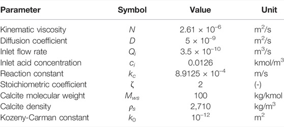
TABLE 1. Simulation parameters for Benchmark 1.

Figure 1 shows the concentration map at different times for the different methods, with c = 0 in the solid phase. We see that for the ALE and iVoS methods, the concentration maps are very similar and the calcite post has fully disappeared at t = 12,000 s. However, for the VoS-ψ method, the dissolution is delayed and there is still a small but significant volume of calcite at t = 12,000 s. The VoS-ψ’ method corrects most of this error and the concentration maps are similar to the one obtained with the ALE and iVoS methods.

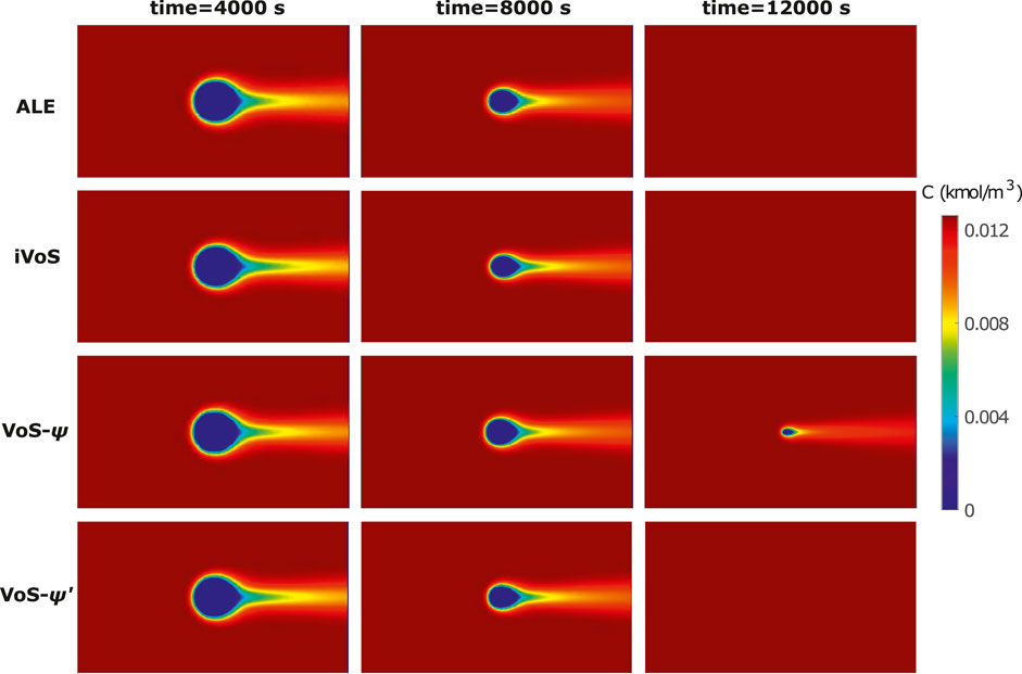
FIGURE 1. Concentration map at various times during dissolution of a calcite post by acid injection using the ALE, VoS-ψ, VoS-ψ’ and iVoS methods.

The results of numerical simulations at different mesh resolutions are compared with experimental results from Soulaine et al. (2017) in Figure 2. We observe that the ALE method converges toward a solution close to the experimental results. The difference between the experimental results and the numerical simulation at mesh resolution Δx = 5 μm in grain volume and grain area are less than 1% of the initial values. Although the iVoS method gives a significantly lower grain volume and surface area than the experiment at a resolution Δx = 20 μm, the results are very similar to the ALE results for Δx = 10 μm and Δx = 5 μm. In addition, with the iVoS method as with the ALE method, the difference between the experimental results and the numerical simulation at mesh resolution Δx = 5 μm in grain volume and grain area are less than 1% of the initial values.

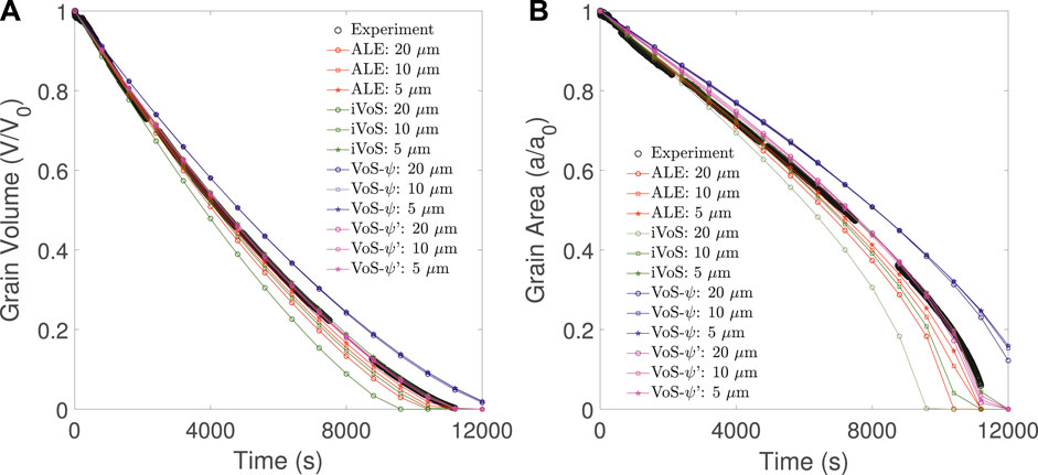
FIGURE 2. Evolution of (A) the grain volume and (B) the grain surface area obtained experimentally (black) and with simulation using the ALE (red), VoS-ψ (blue),, VoS-ψ’ (purple) and iVoS (green) methods at various mesh resolutions during dissolution of a calcite post by acid injection.

Although the VoS-ψ method matches the trend of the experiment, it overestimates the grain volume and surface area for all resolutions. The results do not improve as the mesh resolution increases and converge toward a solution with an error of 5% in the grain volume and 10% in the grain area. This error is corrected by the surface area correction provided by the VoS-ψ′ method. At all resolution, the VoS-ψ’ method gives errors in grain volume and grain area that are less than 1% of the initial values. During the simulation, λ_ɛ is a value between 8 and 16 that changes as ɛ changes. This shows that the VoS-ψ underestimates the overall surface area by a factor between 2 and 4.

Table 2 shows the CPU times for all simulations. The simulations are significantly faster using the VoS methods, with the iVoS being approximately 2.5x faster than the ALE for each simulation. For Δx = 20 μm and Δx = 10 μm, the VoS-ψ method is slightly faster than the iVoS and VoS-ψ′ methods, which is due to the larger time steps (average of 2.1 s for VoS-ψ compared to 1.7 s for iVoS and VoS-ψ′ for the simulation with Δx = 10 μm) and a faster convergence of the steady-state solver (average of six iterations per time-step for VoS-ψ compared to seven iterations for iVoS and VoS-ψ’ for the simulation with Δx = 10 μm). These differences disappear for the simulation with Δx = 5 μm.

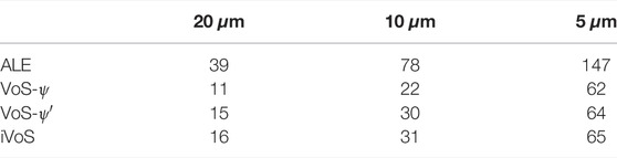
TABLE 2. CPU time [min] obtained with the ALE, VoS-ψ, VoS-ψ’ and iVoS methods at various mesh resolutions during dissolution of a calcite post by acid injection.

We conclude that all VoS methods are significantly faster than the ALE method. The iVoS provides a result that converges toward a solution with an error less than 1% when the mesh resolution reaches 5 μm. The VoS-ψ results in a small error which is due to the reduction of the overall surface area and is corrected in the VoS-ψ′ method by fitting the constant λ for each time-step. The VoS-ψ’ method gives accurate results for all mesh resolution.

3.2 Benchmark 2: Dissolution Regimes in a 2D Model

In benchmark 2, we use the three VoS methods to model the various dissolution regimes (i.e compact, wormholes, and uniform) that occur during mineral dissolution in a 2D porous media model. ALE simulations are also run for reference. The model is constructed from a homogeneous domain with discs radius 270 μm by adding a random deviation of magnitude 270 μm in disc radius and center position. The micromodel generation code is available open source (https://github.com/hannahmenke/DrawMicromodels) and the method is described in Patsoukis-Dimou et al. (2021). The geometry is presented in Figure 3 and a high resolution image can be found in the Supplementary Material.

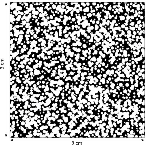
FIGURE 3. Micromodel geometry for Benchmark 2.

The domain is meshed with a Cartesian mesh with uniform resolution Δx = 3 μm, which is snapped on the solid surfaces for the ALE method. A band of 2 cells width is added on each side of the model to avoid dissolution at the boundaries. The final meshes include 1,008,016 cells for the VoS methods and 457,455 for the ALE method. The porosity ϕ and the permeability K of the full domain can be numerically calculated as ϕ = 0.45 and K = 5.6 × 10^–10 m².

At t = 0, acid is injected from the left boundary at constant flow rate, extrapolated from a zero-gradient pressure velocity field (OpenCFD, 2016), and flows out of the domain from the right boundary at constant pressure. The top and bottom boundaries are no-flow, no-slip conditions. The fluid and solid properties are summarized in Table 3. The Kozeny-Carman constant is fitted to obtain the same permeability as in the direct method at t = 0. For each simulation, the inlet flow rate Q_i and the chemical reaction constant k_c are adapted to obtain the correct Pe and Ki, using the pore-scale length $L=\sqrt{12K/\varphi }$ as the reference length and the average pore velocity U = U_D/ϕ as the reference velocity. The factor 12 is added so that the pore-scale length corresponds to the channel size for an homogeneous bundle of straight channels (Pavuluri et al., 2018). Four cases are considered that characterize four different dissolution regimes: Pe = 0.01 and Ki = 0.1 (compact dissolution), Pe = 0.3 and Ki = 10 (conical wormhole), Pe = 1 and Ki = 1 (dominant wormhole), and Pe = 10 and Ki = 0.01 (uniform dissolution). The simulations are performed until 20% of the solid has been dissolved.

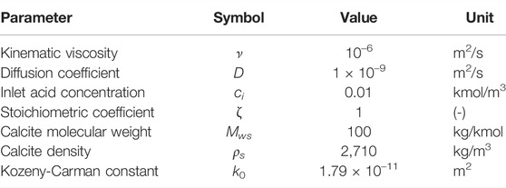
TABLE 3. Simulation parameters for Benchmark 2.

Figure 4 shows the concentration map at the end of the simulations. We observe that all methods are able to model all regimes qualitatively. In particular, the iVoS method reproduces the ALE results almost exactly. However, there are several inaccuracies in the VoS-ψ method. Due to the use of a centered scheme for the computation of the gradient of ɛ, the VoS-ψ method results in several grains with incomplete dissolution in the compact and wormhole regimes. This problem can be resolved by applying a decentered gradient, but this is done at the expense of accuracy, as a decentered gradient generates more numerical diffusion. In addition, the wormhole obtained with VoS-ψ for Pe = 1 and Ki = 1 is more diffused and ramified that the ones obtained with ALE and iVoS, due to the reduction of reaction rate induced by ψ. For the uniform regime, the patterns are almost identical, but the acid concentration obtained with the VoS-ψ method is higher than with ALE and iVoS, suggesting that the reaction rate is lower for VoS-ψ. Most of these errors are corrected in the VoS-ψ’ method, although there are still grains with incomplete dissolution in the compact and wormhole regime, and the wormhole is still slightly more diffuse and ramified for Pe = 1 and Ki = 1.

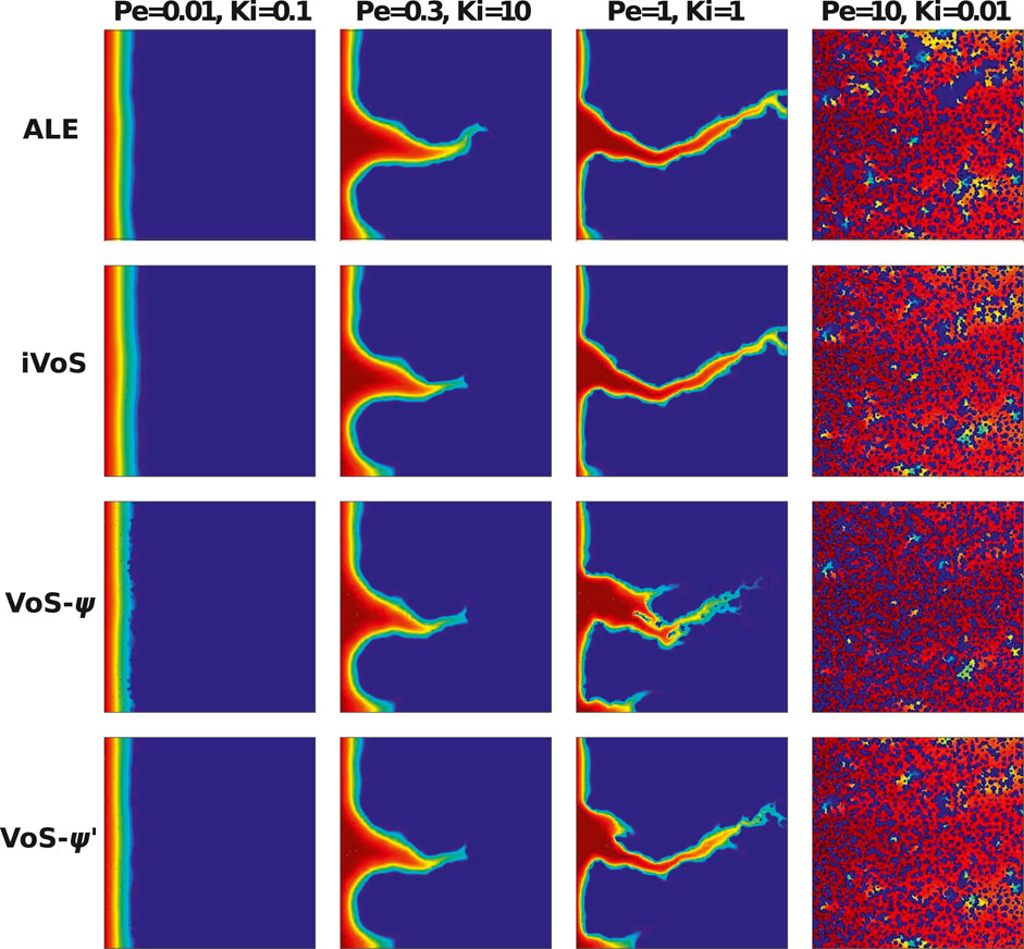
FIGURE 4. Acid concentration map after 20% dissolution in a micromodel for four different regimes (Benchmark 2) obtained by numerical simulations.

Figures 5, 6 show the evolution of the solid volume and solid surface area for all regimes obtained with all numerical methods. We observe that the iVoS method reproduces the ALE results with good accuracy for all regimes. For all cases, the solid volume and surface area evolutions obtained with the ALE and the iVoS methods are similar. The VoS-ψ method underpredicts the amount of dissolution occurring in the systems compared to the ALE and the iVoS methods. This is particularly true for the cases with Ki ≤ 0.1, i.e. in the compact and uniform regime. In these cases, the concentration gradient on the reactive surface is small and the reaction rate is mostly dependent on the surface area, which is significantly reduced by the localization function ψ. For the dominant wormhole regime, although the solid volume evolution obtained with the VoS-ψ method is similar to the ones obtained with the ALE and iVoS methods, the evolution of the solid area is significantly different. This suggests that, although the total amount of dissolution is correctly predicted, it occurs in a slightly different pattern than with the ALE and iVoS methods. The dissolution front is less sharp, and the reaction occurs in the vicinity of the wormhole rather than at the tip of the wormhole as predicted by the ALE and iVoS methods. This leads to a more ramified dissolution pattern, as observed in Figure 4. The VoS-ψ’ method corrects some of these errors and the overall amount of dissolution is similar to the ALE and iVoS results for all cases. However, the surface area is slightly higher for all cases. This is because, since the dissolution is high when ɛ ≈ 0.5 and low when ɛ ≈ 0 and ɛ ≈ 1, the interface becomes artificially sharp and leads to a larger interfacial area.

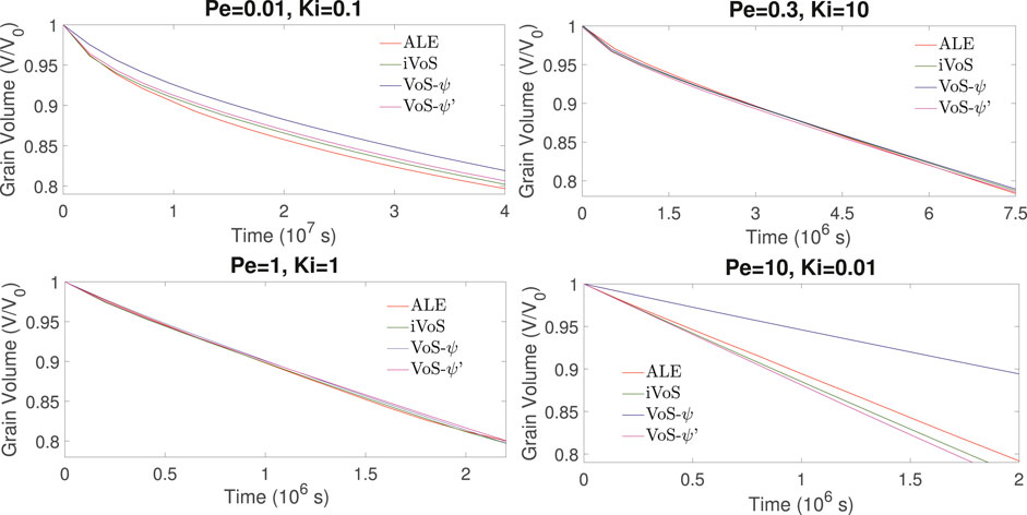
FIGURE 5. Evolution of the solid volume during numerical simulation of dissolution in a 2D micromodel at four different regimes.

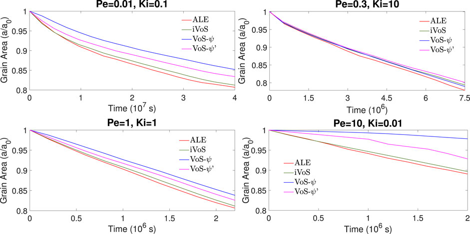
FIGURE 6. Evolution of the solid surface area during numerical simulation of dissolution in a 2D micromodel at four different regimes.

Figure 7 shows the evolution of the permeability K and the correction factor α as a function of porosity for all regimes obtained with the four methods. In all cases, the order of the permeability evolution is similar for the three methods, except for the dominant wormhole regime, for which the order is 19 for ALE and 17 for iVoS, typical of the dominant wormhole regime, but only 8 for VoS-ψ and 12 for VoS-ψ′, which is more typical of the ramified wormhole regime. Compared to the ALE method, the difference of permeability (in log scale) at the end of the simulation is 13% for the iVoS method, 40% for the VoS-ψ′ method and 60% for the VoS-ψ method. The macro-scale reaction constant is consistently lower with VoS-ψ than with ALE and iVoS, especially for the uniform regime where the difference with the ALE result at the end of the simulation is 2% for the iVoS method, 8% for the VoS-ψ’ method and 78% for the VoS-ψ method.

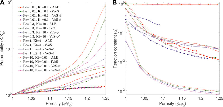
FIGURE 7. Evolution of the permeability and macro-scale reaction constant during numerical simulation of dissolution in a 2D micromodel at four different regimes obtained with the ALE, the (A) VoS-ψ and the (B) iVoS methods.

Table 4 shows the CPU time for all cases for all three methods. We observe that the VoS methods are between 3 and 12 time faster than the ALE method. The VoS methods are particularly efficient compared to the ALE method for the cases with localized dissolution front, i.e., for the compact and the wormholing regime, for which the ALE method performs a large number of remeshing steps. The VoS-ψ method is slightly faster than the iVoS method, but this is mostly due to larger time steps resulting from the lower dissolution rates. The VoS-ψ’ method is slightly slower than the iVoS method, which we attribute to a slower convergence of the transport equation due to a more localized dissolution.

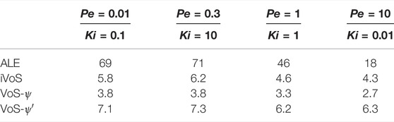
TABLE 4. CPU time (in hours) obtained for all three methods for all four regimes during dissolution in a 2D micromodel.

We conclude that the iVoS method is capable of modelling all regimes during dissolution in a 2D micromodel and calculating macro-scale coefficients with similar results as the ones obtained with ALE. In addition, the iVoS method is significantly faster than the ALE method. The VoS-ψ method, using ψ = 4ɛ_f (1 − ɛ_f) underpredicts the dissolution in all cases due to a reduction of overall surface area, but this error is mostly corrected by using the VoS-ψ’ method.

3.3 Benchmark 3: Dissolution in a 3D Micro-CT Image and Comparison With Experiment

In benchmark 3 we simulate the dissolution of a 3D micro-CT image of Ketton limestone and compare the numerical results to in-situ dissolution experiments. The main advantage of the micro-continuum approach is its computational efficiency compared to the ALE method. In this part, we take advantage of this to perform simulations with a VoS method, while the ALE method is too computationally expensive to perform on a 3D image of this size. The iVoS method was selected since it gave the most accurate results in benchmark 2. The experiment is the one conducted in Menke et al. (2015), where CO₂-saturated brine is injected in a Ketton carbonate core. A core of 4 mm diameter was flooded with a brine solution representative of a typical saline aquifer consisting of 1% KCl and 5% NaCl by weight, pre-equilibrated with supercritical CO₂ at 10 MPa and 50 C. Micro-CT images were acquired after 17, 33, 50 and 67 min.

The simulated conditions are similar to the ones presented in Pereira Nunes et al. (2016). The sample is a cylinder of radius 1.7 mm and length 3.5 mm. The image has 911 × 902 × 922 voxels with resolution 3.8 μm, however, we ran it on two-level adpative mesh with maximum resolution of 7.6 μm to decrease computation time. The initial grid includes 17 million cells. Figure 8A shows the initial porosity field. The velocity field is then initialised by solving Equ. 17) and 11) in the domain using k₀ = 2 × 10^–13 m² which was fitted to obtain a permeability of 16D. The streamlines and corresponding magnitude of velocity are shown on Figure 8B. The reaction rate is described in terms of the concentration of calcium cations Ca²⁺, following $R=k_{\mathit{eff}}\left(C_{eq}-C\right)$, where C_eq and k_eff depend on the concentrations of $C{O}_3^{2-}$, H⁺ and C O ₂. Because our model only tracks one component, the reaction constant and equilibrium concentration are fitted to match the reaction-limited constant obtained for a flat pure crystal of calcite (Peng et al., 2015) R = 8.1 × 10^–7 kmol/m²/s and the initial reaction rate in the experiment R = 8.8 × 10^–8 kmol/m²/s. Such rates are obtained using a reactant concentration of 0.0035 kmol/m³ at the inlet and a reaction constant k_c = 2.314 × 10^–4 m/s. Figure 8C shows the concentration field in the pores at T = 0 s obtained by solving Equ. (A.4).

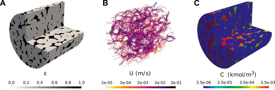
FIGURE 8. Initial condition for simulation of dissolution in a 3D micro-CT image of carbonate: (A) initial local porosity field; (B) Initial calculated velocity field; (C) Initial calculated concentration field (Pe =190, Da =4.4×10^–2).

The simulation parameters are summarized in Table 5. We use for reference velocity the average pore velocity defined as

The reference length is associated to the initial permeability so that

where the constant 8 is added in order to obtain the throat radius for a capillary bundle of uniform size. With these definitions, we obtain U = 5.3 × 10^–3 m/s and L = 27 μm. Using the diffusion coefficient and reaction constant in Table 5, we obtain Pe = 190 and Da = 4.4 × 10^–2.

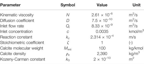
TABLE 5. Simulation parameters for Benchmark 3.

The simulation is run with an adaptive time-step until t = 4,000 s on 128 CPUs using Oracle cloud computing. The total CPU time was 65 h. Figure 9 shows a comparison of the evolution of the dissolution pattern between experiment and simulation. The colors show the part of the rock that is dissolved for each time interval. We observe that the simulation captures the correct patterns, with pores being enlarged in the direction of the flow. Some expected differences are observed, primarily due to uncertainties in the experimental conditions, segmentation error due to reaction occurring during image acquisition, and the fact that the simulation is performed on a sub-image of the full sample used in the experiment. Furthermore, some of the differences in the local porosity at different times in the experiment are due to imperfect alignment of the images. Table 6 shows the evolution of the porosity during dissolution for both experiment and simulation. We observe that the porosity is accurately predicted by the simulation until T > 3,000 s, at which time the simulation starts diverging from the experiment slightly. This can be explained by the fact that the simulation is done on a sub-image of the full sample, starting at 2 mm away from the inlet (Menke et al., 2015), and thus the concentration of acid will have varied as dissolution occured in the unimaged portion of the core.

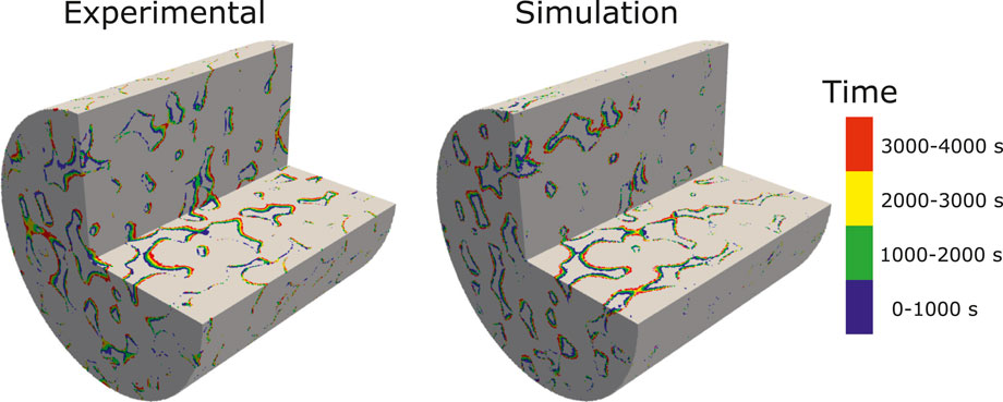
FIGURE 9. Experimental and simulated results showing the evolution of the dissolution pattern in a 3D micro-CT image of Ketton Carbonate. The colors represent different time intervals.

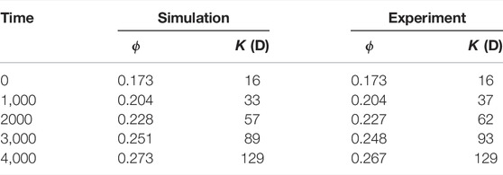
TABLE 6. Experimental and simulated porosity and permeability at different time during dissolution in a 3D micro-CT image of Ketton Carbonate.

In addition, permeability can be calculated during the simulation. Table 6 shows the porosity and permeability at different times for the simulation and the experiment and we observe a good correspondence. The permeability is then plotted as a function of the porosity in Figure 10. We see that the permeability in the simulation follows the same trend that of the experiment. Finally, the average macro-scale reaction rate for each time interval can be calculated as

for both simulation and experiment. The correction factor α can then be calculated by dividing by the average concentration in the pore space, calculated at the end of the time interval from the simulation results. The values are summarized in Table 7. We observe a good correspondence between simulation and experiment. The overall trend of decreasing reaction rates and correction factors observed in the experiment is reproduced in the simulation, albeit with a slightly slower rate. This decrease is not a typical characteristic of the uniform regime, and is an indication that the dissolution might be occuring in the channeling regime, identified in Menke et al. (2017).

FIGURE 10. Permeability as a function of evolving porosity during dissolution in a 3D micro-CT image of Ketton Carbonate.

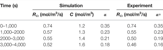
TABLE 7. Evolution of experimental and simulated reaction rate, reactant concentration and macro-scale reaction constant. The experimental macro-scale constant α* is calculated using the simulated concentration.

Two additional simulations are run in different regimes by dividing the reaction rate by 100 and 10,000, which gives Péclet number of 1.9 and 0.019. The simulations are run on 128 CPUs using Oracle cloud computing until the porosity reaches an approximate value of 0.28. The CPU time was 75 h for Pe = 1.9 and 80 h for Pe = 0.019. Figure 11 shows the reactant concentration along reconstructed streamlines at the end of the simulation. At Pe = 0.019, the dissolution is in the compact regime. The reactant is consumed and dissolves the rock close to the inlet face. At Pe = 1.9, the dissolution is in the wormholing regime. The reactant penetrates further in the domain and flow instabilities kick in, leading to a preferential dissolution pathway. The streamlines and reactant concentration for Pe = 190 are also shown in Figure 11 and the dissolution appears to be in the uniform regime.

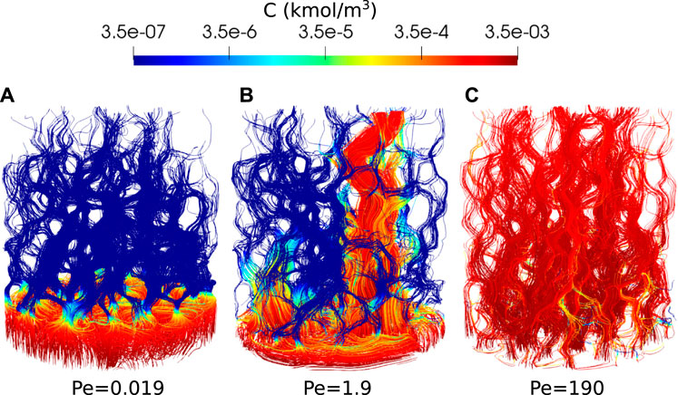
FIGURE 11. Reactant concentration along streamlines during Ketton dissolution in three different regimes, [(A): Pe=0.019, (B): Pe=1.9 and (C): Pe=190] shown when the porosity has reached approximatively 0.28.

Figure 12A shows the evolution of permeability as a function of porosity during the simulations for the three regimes. The permeability of the compact and uniform can be fitted with power laws, and we obtain K = 30ϕ^0.36 for the compact regime and K = 5.5 × 10⁴ϕ^4.7 for the uniform regime. For the wormhole regime, the permeability curve has a strong inflection point around ϕ = 0.25, which corresponds to porosity at reactant breakthrough time. This is typical of the wormholing regime. Before breakthrough occurs, the wormhole does not provide a connected pathway throughout the sample, so the permeability increases with low order. When acid reaches the outlet, the sample becomes fully connected by the wormhole and the permeability increases with high order. The permeability curve can then be fitted with two power law curves, K = 74ϕ^2.1 before breakthrough and K = 3.4 × 10¹⁰ϕ¹⁵ after breakthrough. The orders of the uniform and wormhole regimes correspond those observed in the literature (Menke et al., 2017).

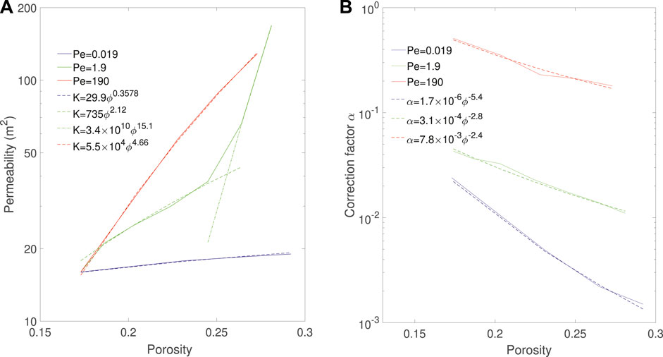
FIGURE 12. Evolution of (A) permeability and (B) correction factor as a function of porosity and corresponding correlations during Ketton dissolution in three different regimes.

Similarly, Figure 12B shows the evolution of the correction factor α as a function of porosity during the simulations for the three regimes. For each regime, the evolution of α can be fitted with a power law (Seigneur et al., 2019) and we obtain α = 1.7 × 10⁻⁶ϕ^−5.4 for the compact regime, α = 3.1 × 10⁻⁴ϕ^−2.8 for the wormholing regime and α = 7.8 × 10⁻³ϕ^−2.4 for the uniform regime. We observe that the correction factor for the uniform regime is not constant but decreases with a power-law. This indicates that the dissolution might not be in the uniform regime, but could be in the channeling regime identified in (Menke et al., 2017).

We conclude that the accuracy and computational efficiency of the iVoS method enables simulation of dissolution in a 3D micro-CT image of a real carbonate sample, reproduce experimental results with good precision and can be used to investigate upscaling parameters.

4 Conclusion

We have presented two novel numerical methods, iVoS and VoS-ψ′, to simulate mineral dissolution in real pore-scale geometries that when compared to existing methods has two main advantages. First, they are based on the micro-continuum approach, and therefore do not require a complex algorithm for interface tracking, nor any special treatment if topological changes occur. Second, the iVoS method calculates a reaction rate based on the divergence of a reactive flux, and thus does not require an interface localization function, which greatly improved its accuracy. The VoS-ψ’ uses a localization function with a constant that is fitted to ensure that the reactive surface area is conserved globally and therefore avoids most of the numerical errors present with VoS-ψ. The advantages of these methods were demonstrated in three benchmark cases.

In benchmark 1, the iVoS method was used to simulate the dissolution of a 3D calcite post in a straight microchannel, and the results were compared with experimental results and with simulations obtained with the ALE method and with the standard micro-continuum approach based on the VoS-ψ method. We observed that the iVoS method was capable of reproducing the experimental results with similar accuracy but significantly less computational time than the ALE method, while the VoS-ψ method using ψ = 4ɛ_f (1 − ɛ_f) showed significantly more error, but this error was corrected by the VoS-ψ’ approach. All VoS methods were significantly faster than the ALE method.

In benchmark 2, we simulated dissolution in a 2D micromodel and calculated macro-scale coefficients using all numerical methods. Four cases in three different dissolution regimes (i.e. compact, wormholing, and uniform) were considered and we observed a qualitative match between the ALE and iVoS simulations, and a good correspondence between the macro-scale coefficients calculated. The iVoS method was between 4 and 12 times faster than the ALE method. The VoS-ψ method using ψ = 4ɛ_f (1 − ɛ_f) was much faster than the ALE method, but underpredicted the dissolution and resulted in inaccurate macro-scale coefficients. Most of these errors were corrected by the VoS-ψ’ approach, but the results were still slightly less accurate than with iVoS.

In benchmark 3, the computational efficiency of the iVoS method was used to perform a simulation in a 3D micro-CT image of a real carbonate rock (i.e., Ketton) and the simulation results were compared to experimental results. We observe a good correspondence between the experimental and simulated results for the evolution of the total porosity change, total reaction rate and permeability with time. Two additional simulations were performed in different dissolution regimes and the accuracy of correlations for macro-scale coefficients evaluated. We observed that the simulated results could be matched by power-law correlations, and that the coefficients obtained for the permeability in the wormhole and uniform regimes correspond to what has been observed in experiments (Menke et al., 2015, 2017).

In future work, the advantages of our novel approach will be used to perform a large number of simulations in 2D micromodels and 3D micro-CT images that will form a large database for data-driven research. This database will then be used to identify precisely the boundaries between the regimes and decipher the impact of pore-scale heterogeneities. Machine-learning algorithms will also be used to estimate macro-scale coefficients in a similar way that for single-phase flow and reactive transport (Menke et al., 2021; Liu et al., 2022) but extended to predict their evolution with the porosity change. Because the micro-continuum approach can also be used to simulate dissolution at the Darcy-scale (Liu et al., 1997; Ormond and Ortoleva, 2000; Golfier et al., 2002), our method can be extended to simulate flow, transport and dissolution in multi-scale porous media (Patsoukis-Dimou et al., 2020). Further, the applicabilities of the methods to model precipitation (Yang et al., 2021) will be investigated, Finally, our approach is compatible with the Volume-Of-Fluid and the Continuous Species Transfer methods (Soulaine et al., 2018) for simulation of multiphase flow and multiphase transport with interfacial transfer, so it has the potential to be extended to simulate mineral dissolution during multiphase processes, which is relevant to a number of clean-energy applications, including CO₂ storage and geothermal systems (Li et al., 2022).

Data Availability Statement

The datasets presented in this study can be found in online repositories. The names of the repository/repositories and accession number(s) can be found in the article/Supplementary Material.

Author Contributions

JM built the models and ran the simulations. JM, CS, and HM designed the research and wrote the paper.

Funding

This work was funded by the Engineering and Physical Sciences Research Council’s grant on Direct Numerical Simulation for Additive Manufacturing (EP/P031307/1).

Conflict of Interest

The authors declare that the research was conducted in the absence of any commercial or financial relationships that could be construed as a potential conflict of interest.

Publisher’s Note

All claims expressed in this article are solely those of the authors and do not necessarily represent those of their affiliated organizations, or those of the publisher, the editors and the reviewers. Any product that may be evaluated in this article, or claim that may be made by its manufacturer, is not guaranteed or endorsed by the publisher.

Supplementary Material

The Supplementary Material for this article can be found online at: https://www.frontiersin.org/articles/10.3389/feart.2022.917931/full#supplementary-material

References

Black, J. R., Carroll, S. A., and Haese, R. R. (2015). Rates of Mineral Dissolution under CO2 Storage Conditions. Chem. Geol. 399, 134–144. doi:10.1016/j.chemgeo.2014.09.020
Chatelin, R., Sanchez, D., and Poncet, P. (2016). Analysis of the Penalized 3d Variable Viscosity Stokes Equations Coupled to Diffusion and Transport. ESAIM M2AN 50, 565–591. doi:10.1051/m2an/2015056
Cooke, J. J., Armstrong, L. M., Luo, K. H., and Gu, S. (2014). Adaptive Mesh Refinement of Gas-Liquid Flow on an Inclined Plane. Comput. Chem. Eng. 60, 297–306. doi:10.1016/j.compchemeng.2013.09.007
Golfier, F., Zarcone, C., Bazin, B., Lenormand, R., Lasseux, D., and Quintard, M. (2002). On the Ability of a Darcy-Scale Model to Capture Wormhole Formation during the Dissolution of a Porous Medium. J. Fluid Mech. 457, 213–254. doi:10.1017/s0022112002007735
Hao, Y., Smith, M., Sholokhova, Y., and Carroll, S. (2013). CO2-induced Dissolution of Low Permeability Carbonates. Part II: Numerical Modeling of Experiments. Adv. Water Resour. 62, 388–408. doi:10.1016/j.advwatres.2013.09.009
Kang, Q., Zhang, D., Chen, S., and He, X. (2002). Lattice Boltzmann Simulation of Chemical Dissolution in Porous Media. Phys. Rev. E 65, 036318. doi:10.1103/PhysRevE.65.036318
Li, P., Deng, H., and Molins, S. (2022). The Effect of Pore-Scale Two-phase Flow on Mineral Reaction Rates. Front. Water 3. doi:10.3389/frwa.2021.734518
Li, X., Huang, H., and Meakin, P. (2010). A Three-Dimensional Level Set Simulation of Coupled Reactive Transport and Precipitation/dissolution. Int. J. Heat Mass Transf. 53, 2908–2923. doi:10.1016/j.ijheatmasstransfer.2010.01.044
Lichtner, P. C. (1988). The Quasi-Stationary State Approximation to Coupled Mass Transport and Fluid-Rock Interaction in a Porous Medium. Geochimica Cosmochimica Acta 52, 143–165. doi:10.1016/0016-7037(88)90063-4
Liu, M., Kwon, B., and Kang, P. K., (2022). Machine Learning to Predict Effective Reaction Rates in 3D Porous Media from Pore Structural Features. doi:10.21203/rs.3.rs-1284059/v1
Liu, X., Ormond, A., Bartko, K., Ying, L., and Ortoleva, P. (1997). A Geochemical Reaction-Transport Simulator for Matrix Acidizing Analysis and Design. J. Petroleum Sci. Eng. 17, 181–196. doi:10.1016/s0920-4105(96)00064-2
Luo, H., Quintard, M., Debenest, G., and Laouafa, F. (2012). Properties of a Diffuse Interface Model Based on a Porous Medium Theory for Solid-Liquid Dissolution Problems. Comput. Geosci. 16, 913–932. doi:10.1007/s10596-012-9295-1
Luquot, L., Rodriguez, O., and Gouze, P. (2014). Experimental Characterization of Porosity Structure and Transport Property Changes in Limestone Undergoing Different Dissolution Regimes. Transp. Porous Med. 101, 507–532. doi:10.1007/s11242-013-0257-4
Maes, J., and Menke, H. P. (2020). “A Bespoke OpenFOAM Toolbox for Multiphysics Flow Simulations in Pore Structures,” in Proceedings of the 17th International Conference on Flow Dynamics. ICFD2020).
Maes, J., and Menke, H. P. (2022). GeoChemFoam: Direct Modelling of Flow and Heat Transfer in Micro-CT Images of Porous Media. Heat. Mass Transf. doi:10.1007/s00231-022-03221-2
Maes, J., and Menke, H. P. (2021a). GeoChemFoam: Direct Modelling of Multiphase Reactive Transport in Real Pore Geometries with Equilibrium Reactions. Transp. Porous Med. 139, 271–299. doi:10.1007/s11242-021-01661-8
Maes, J., and Menke, H. P. (2021b). GeoChemFoam: Operator Splitting Based Time-Stepping for Efficient Volume-Of-Fluid Simulation of Capillary-Dominated Two-phase Flow. arXiv:2105.10576 arXiv:2105.10576.
Maes, J., and Soulaine, C. (2020). A Unified Single-Field Volume-Of-Fluid-Based Formulation for Multi-Component Interfacial Transfer with Local Volume Changes. J. Comput. Phys. 402, 109024. doi:10.1016/j.jcp.2019.109024
Menke, H. P., Andrew, M. G., Blunt, M. J., and Bijeljic, B. (2016). Reservoir Condition Imaging of Reactive Transport in Heterogeneous Carbonates Using Fast Synchrotron Tomography - Effect of Initial Pore Structure and Flow Conditions. Chem. Geol. 428, 15–26. doi:10.1016/j.chemgeo.2016.02.030
Menke, H. P., Bijeljic, B., Andrew, M. G., and Blunt, M. J. (2015). Dynamic Three-Dimensional Pore-Scale Imaging of Reaction in a Carbonate at Reservoir Conditions. Environ. Sci. Technol. 49, 4407–4414. doi:10.1021/es505789f
Menke, H. P., Bijeljic, B., and Blunt, M. J. (2017). Dynamic Reservoir-Condition Microtomography of Reactive Transport in Complex Carbonates: Effect of Initial Pore Structure and Initial Brine pH. Geochimica Cosmochimica Acta 204, 267–285. doi:10.1016/j.gca.2017.01.053
Menke, H. P., Maes, J., and Geiger, S. (2021). Upscaling the Porosity-Permeability Relationship of a Microporous Carbonate for Darcy-Scale Flow with Machine Learning. Sci. Rep. 11. doi:10.1038/s41598-021-82029-2
Menke, H. P., Reynolds, C. A., Andrew, M. G., Pereira Nunes, J. P., Bijeljic, B., and Blunt, M. J. (2018). 4D Multi-Scale Imaging of Reactive Flow in Carbonates: Assessing the Impact of Heterogeneity on Dissolution Regimes Using Streamlines at Multiple Length Scales. Chem. Geol. 481, 27–37. doi:10.1016/j.chemgeo.2018.01.016
Molins, S., Soulaine, C., Prasianakis, N. I., Abbasi, A., Poncet, P., Ladd, A. J. C., et al. (2020). Simulation of Mineral Dissolution at the Pore Scale with Evolving Fluid-Solid Interfaces: Review of Approaches and Benchmark Problem Set. Comput. Geosci. 25, 1285–1318. doi:10.1007/s10596-019-09903-x
Molins, S., Trebotich, D., Miller, G. H., and Steefel, C. I. (2017). Mineralogical and Transport Controls on the Evolution of Porous Media Texture Using Direct Numerical Simulation. Water Resour. Res. 53, 3645–3661. doi:10.1002/2016wr020323
Nogues, J., Fitts, J., Celia, A. M., and Peters, C. (2013). Permeability Evolution Due to Dissolution and Precipitation of Carbonates Using Reactive Transport Modeling in Pore Networks. Water Resour. Res. 49. doi:10.1002/wrcr.20486
Noiriel, C., Luquot, L., Raimbault, L., Gouze, P., and Van Der Lee, J. (2009). Changes in Reactive Surface Area during Limestone Dissolution: An Experimental and Modelling Study. Chem. Geol. 265, 160–170. doi:10.1016/j.chemgeo.2009.01.032
Nordbotten, J. M., and Celia, M. A. (2011). Geological Storage of CO2: Modeling Approaches for Large-Scale Simulation. John Wiley & Sons.
Ormond, A., and Ortoleva, P. (2000). Numerical Modeling of Reaction-Induced Cavities in Porous Rock. J. Geophys. Res. 105 (16737–16), 747. doi:10.1029/2000jb900116
Palmer, A. N. (1991). Origin and Morphology of Limestone Caves. Geol. Soc. Am. Bull. 103, 1–21. doi:10.1130/0016-7606(1991)103<0001:oamolc>2.3.co;2
Pandey, S. N., Chaudhuri, A., Rajaram, H., and Kelkar, S. (2015). Fracture Transmissivity Evolution Due to Silica Dissolution/precipitation during Geothermal Heat Extraction. Geothermics 57, 111–126. doi:10.1016/j.geothermics.2015.06.011
Parkhurst, D. L., and Wissmeier, L. (2015). Phreeqcrm: A Reaction Module for Transport Simulators Based on the Geochemical Model Phreeqc. Adv. Water Resour. 83, 176–189. doi:10.1016/j.advwatres.2015.06.001
Patsoukis Dimou, A., Menke, H. P., and Maes, J. (2021). Transport in Porous Media, 141, 279–294. doi:10.1007/s11242-021-01718-8Benchmarking the Viability of 3D Printed Micromodels for Single Phase Flow Using Particle Image Velocimetry and Direct Numerical SimulationsTransp. Porous Med.
Patsoukis-Dimou, A., Suzuki, A., Menke, H. P., Geiger, S., and Maes, J. (2020). “3D Printing-Based Microfluidics for Geosciences,” in Proceedings of the 18th International Conference on Flow Dynamics. ICFD2021).
Pavuluri, S., Maes, J., and Doster, F. (2018). Spontaneous Imbibition in a Microchannel: Analytical Solution and Assessment of Volume of Fluid Formulations. Microfluid Nanofluid 22. doi:10.1007/s10404-018-2106-9
Peng, C., Crawshaw, J. P., Maitland, G. C., and Trusler, J. P. M. (2015). Kinetics of Calcite Dissolution in CO2-saturated Water at Temperatures between (323 and 373) K and Pressures up to 13.8 MPa. Chem. Geol. 403, 74–85. doi:10.1016/j.chemgeo.2015.03.012
Pereira Nunes, J. P., Blunt, M. J., and Bijeljic, B. (2016). Pore‐scale Simulation of Carbonate Dissolution in Micro‐CT Images. J. Geophys. Res. Solid Earth 121, 558–576. doi:10.1002/2015jb012117
Prasianakis, N., and Ansumali, S. (2011). Microflow Simulations via the Lattice Boltzmann Method. Commun. Comput. Phys. 9, 1128–1136. doi:10.4208/cicp.301009.271010s
Quintard, M., and Whitaker, S. (1994). Convection, Dispersion, and Interfacial Transport of Contaminants: Homogeneous Porous Media. Adv. Water Resour. 17, 116–126. doi:10.1016/0309-1708(94)90002-7
Raoof, A., Nick, H. M., Hassanizadeh, S. M., and Spiers, C. J. (2013). PoreFlow: A Complex Pore-Network Model for Simulation of Reactive Transport in Variably Saturated Porous Media. Comput. Geosciences 61, 160–174. doi:10.1016/j.cageo.2013.08.005
Seigneur, N., Mayer, K. U., and Steefel, C. I. (2019). Reactive Transport in Evolving Porous Media. Rev. Mineralogy Geochem. 85, 197–238. doi:10.2138/rmg.2019.85.7
Shafiq, M. U., and Mahmud, H. B. (2017). Sandstone Matrix Acidizing Knowledge and Future Development. J. Pet. Explor Prod. Technol. 7, 1205–1216. doi:10.1007/s13202-017-0314-6
Shapiro, M., and Brenner, H. (1988). Dispersion of a Chemically Reactive Solute in a Spatially Periodic Model of a Porous Medium. Chem. Eng. Sci. 43 (3), 551–571. doi:10.1016/0009-2509(88)87016-7
Soulaine, C., Creux, P., and Tchelepi, H. A. (2019). Micro-continuum Framework for Pore-Scale Multiphase Fluid Transport in Shale Formations. Transp. in Porous Med. 127 , 85–112
Soulaine, C., Maes, J., and Roman, S. (2021a). Computational Microfluidic for the Geosciences. Front. Water 3. doi:10.3389/frwa.2021.643714
Soulaine, C., Pavuluri, S., Claret, F., and Tournassat, C. (2021b). porousmedia4foam: Multi-Scale Open-Source Platform for Hydrogeochemical Simulations with Openfoam. Environ. Model. Softw. 145. doi:10.1016/j.envsoft.2021.105199
Soulaine, C., Roman, S., Kovscek, A., and Tchelepi, H. A. (2018). Pore-scale Modelling of Multiphase Reactive Flow: Application to Mineral Dissolution with Production of. J. Fluid Mech. 855, 616–645. doi:10.1017/jfm.2018.655
Soulaine, C., Roman, S., Kovscek, A., and Tchelepi, H. (2017). Mineral Dissolution and Wormholing from a Pore-Scale Perspective. J. Fluid Mech. 827. doi:10.1017/jfm.2017.499
Soulaine, C., and Tchelepi, H. A. (2016). Micro-continuum Approach for Pore-Scale Simulation of Subsurface Processes. Transp. Porous Med. 113, 431–456. doi:10.1007/s11242-016-0701-3
Starchenko, V., and Ladd, A. J. C. (2018). The Development of Wormholes in Laboratory‐Scale Fractures: Perspectives from Three‐Dimensional Simulations. Water Resour. Res. 54, 7946–7959. doi:10.1029/2018wr022948
Starchenko, V., Marra, C. J., and Marra, C., L. A. J. (2016). Three-dimensional Simulations of Fracture Dissolution. J. Geophys. Res. Solid Earth 121, 6421–6444. doi:10.1002/2016jb013321
Steefel, C. I., Appelo, C. A. J., Arora, B., Jacques, D., Kalbacher, T., Kolditz, O., et al. (2015). Reactive Transport Codes for Subsurface Environmental Simulation. Comput. Geosci. 19, 445–478. doi:10.1007/s10596-014-9443-x
Szymczak, P., and Ladd, A. J. C. (2012). Reactive Infiltration Instabilities in Rocks. Fracture Dissolution. J. Fluid Mech. 702, 239–264. doi:10.1017/jfm.2012.174
Szymczak, P., and Ladd, A. J. C. (2009). Wormhole Formation in Dissolving Fractures. J. Geophys. Res. Solid Earth 114. doi:10.1029/2008jb006122
Tartakovsky, A. M., Meakin, P., Scheibe, T. D., and Eichler West, R. M. (2007). Simulations of Reactive Transport and Precipitation with Smoothed Particle Hydrodynamics. J. Comput. Phys. 222, 654–672. doi:10.1016/j.jcp.2006.08.013
van Leer, B. (1974). Towards the Ultimate Conservative Difference Scheme. II. Monotonicity and Conservation Combined in a Second-Order Scheme. J. Comput. Phys. 14, 361–370. doi:10.1016/0021-9991(74)90019-9
Varloteaux, C., Bekri, S., and Adler, P. M. (2013). Pore Network Modelling to Determine the Transport Properties in Presence of a Reactive Fluid: from Pore to Reservoir Scale. Adv. Water Resour. 53, 87–100. doi:10.1016/j.advwatres.2012.10.004
Walsh, S. D. C., Garapati, N., Leal, A. M. M., and Saar, M. O. (2013). Calculating Thermophysical Fluid Properties during Geothermal Energy Production with Ness and Reaktoro. Geothermics 70, 146–154.
Wen, H., and Li, L. (2017). An Upscaled Rate Law for Magnesite Dissolution in Heterogeneous Porous Media. Geochimica Cosmochimica Acta 210, 289–305. doi:10.1016/j.gca.2017.04.019
Williams, B. B., Gidley, J. L., and Schechter, R. S. (1979). Acidizing Fundamentals. Society of Petroleum Enginners.
Yang, F., Stack, G. A., and Starchenko, V. (2021). Micro-continuum Approach for Mineral Precipitation. Sci. Rep. 11. doi:10.1038/s41598-021-82807-y
Keywords: pore-scale, reactive transport, micro-continuum, OpenFOAM, dissolution
Citation: Maes J, Soulaine C and Menke HP (2022) Improved Volume-Of-Solid Formulations for Micro-Continuum Simulation of Mineral Dissolution at the Pore-Scale. Front. Earth Sci. 10:917931. doi: 10.3389/feart.2022.917931
Received: 11 April 2022; Accepted: 25 May 2022;
Published: 15 July 2022.
Edited by:
Yongfei Yang, China University of Petroleum , ChinaCopyright © 2022 Maes, Soulaine and Menke. This is an open-access article distributed under the terms of the Creative Commons Attribution License (CC BY). The use, distribution or reproduction in other forums is permitted, provided the original author(s) and the copyright owner(s) are credited and that the original publication in this journal is cited, in accordance with accepted academic practice. No use, distribution or reproduction is permitted which does not comply with these terms.
*Correspondence: Julien Maes, j.maes@hw.ac.uk