Power-to-Syngas: A Parareal Optimal Control Approach

1 Introduction

In the context of energy transition towards carbon-free drivers for the chemical and fuel industry, electricity from renewable sources plays a primary role. Availability constraints are associated with the use of renewable electrical power. Engeland et al. (2017) introduced the notion of climate related energy (CRE), which encompasses wind-, solar-power and, partly, hydro-power. Typically, its intermittent provision on the daily and hourly time-scale is attributable to the temporal trends of the related natural source and other factors, such as wind velocity, solar radiation, and atmospheric precipitation. The intermittent nature of the supply as well as the consumer demand contribute to price volatility. As reported by Schill (2014), positive residual power loads in the grid occur whenever demand exceeds the generation of CRE.

Currently, by means of relatively flexible operations and proper forecasts, state-of-the-art power plants can adjust their outputs to meet market demands and manage fluctuations in the provision of renewable power. Reservoir-type hydro-power, i.e., conversion of surplus electricity into potential energy by pumping water into elevated basins, can also contribute to this strategy. Nevertheless, the number of such reservoirs is limited due to morphological constraints. Moreover, as reported in Sinn (2017), seasonal fluctuations are expected to require most of the storage capacity if the share of renewable electricity was to become predominant.

In this framework, Power-to-X processes are relevant contributors to the energy transition: they are conceived to take advantage of unsteady power inputs, thus transformed into valuable chemicals and energy vectors. In particular, as highlighted in a review article by Wulf et al. (2020), the role of H₂ is of cardinal importance in the conversion of electricity. As a matter of fact, projects and industrial applications related to water electrolysis (EL) of increasing capacities are expected in the near future. This contribution shall focus on Power-to-Syngas towards Fischer-Tropsch, for which a molar ratio H₂/CO of 2 must be ensured. H₂ and CO₂ can be converted to syngas via the reverse water-gas shift reaction in a non-adiabatic fixed-bed reactor (RWGS), possibly supported by a number of candidate catalysts, as thoroughly reviewed by Daza and Kuhn (2016). Its mild endothermicity allows for a moderate thermal input to sustain the generation of CO from CO₂.

As the inherent complexity of a tri-phase Fischer-Tropsch synthesis reactor benefits from a steady syngas supply, short-term, e.g., hourly, intermittency could be levelized via H₂ buffering, although resulting in higher investment and operating costs in terms of EL volumes and electricity supply. As an example, if the power load required to attain the nominal flowrate of syngas is 50 MW, 10 wind turbines of 5 MW each would fulfill the duty. Nevertheless, a seasonal shortage of renewable power would require the installation of X additional turbines and a dedicated buffering system for the storage of H₂. Furthermore, Kaiser et al. (2013) report on the high energy intensity required for H₂ liquefaction, amounting up to 30% of its lower heating value, and on its low density, both in gaseous and liquefied state. Moreover, buffering may not guarantee sufficient productivity levels over long term, e.g., seasonal, shortage of renewable power supply. Besides H₂, EL generates O₂ which could be used to sustain the endothermicity of RWGS. Assuming that the thermal duty of RWGS equals its standard enthalpy of reaction (35.3 kJ${\mathrm{m}\mathrm{o}\mathrm{l}}_{\mathrm{C}\mathrm{O}}^{-1}$ at 950 K), resulting in a conversion of 42.7% of an equimolar feed mixture in isothermal operations and for the lower heating value (LHV) of CH₄ (800 kJ mol⁻¹), 0.0882 ${\mathrm{m}\mathrm{o}\mathrm{l}}_{{\mathrm{O}}_2}$ per mole of CO produced are required for heat generation. EL generates 1.5 ${\mathrm{m}\mathrm{o}\mathrm{l}}_{{\mathrm{O}}_2}$${\mathrm{m}\mathrm{o}\mathrm{l}}_{\mathrm{C}\mathrm{O}}^{-1}$ if a syngas ratio H₂/CO of 2 is to be attained. Consequently, 94.1% of the O₂ produced within the plant does not contribute to the generation of syngas. In conclusion, the large majority of O₂ is not utilized within the process: even if the stabilization of syngas were attained via H₂ storage strategies, it would be reasonable to consider O₂ as a valuable by-product to be stored within suitable buffering devices in the plant.

Another route to syngas is tri-reforming of methane (TRI), traditionally meant to convert combustion off-gases and natural gas within a catalytic, adiabatic reactor fed with oxygen or air, as in Song and Pan (2004). The oxidation of CH₄ contributes to lower the levels of carbon deposition and to allow for a tunable outlet composition (Vita et al. (2018)). Biogas from anaerobic digestion and CO₂ can partially or completely substitute the traditional feedstock. The use of O₂ results in high adiabatic temperature peaks although, if compared with air, it requires smaller process volumes and separation costs.

Considering the aforementioned possible downsides of H₂ buffering and the possibility to use a TRI reactor, this contribution proposes the combined implementation of a RWGS and a TRI reactor as an alternative to a H₂ buffering strategy. Here, O₂ is provided either directly from the EL or indirectly, as suitable storage devices are assumed after the splitting of water. If the stored O₂ were not sufficient to feed TRI on a seasonal basis, it could be used to enrich air, then fed to the reactor. In order to ensure a steady syngas supply at the specified H₂/CO molar ratio of 2 under variable electricity provision, the continuous switching between RWGS and TRI operations should be enforced via appropriate control strategies.

After the introduction of modeling assumptions and reactor models, design parameters and operating conditions for the reactors are identified. Afterwards, the overall optimal control strategy is outlined where the final goal is to meet syngas specifications under a time-varying electricity supply. From the mathematical side, parareal shall be employed to speed up expensive model evaluations during the solution of the optimization problems. parareal, see, e.g., Lions et al. (2001); Baffico et al. (2002), aims at decomposing the global time domain into several smaller domains and, given initial values on these subdomains, the global problem splits up into local subproblems that, in each iteration, can be solved in parallel. The initial values are generated using a cheap but possibly inaccurate coarse time integrator and the subproblems are then solved in parallel using an expensive but accurate fine time integrator. Initial values for the next iteration are generated in a correction step utilizing the information from the fine integrator. The derivatives of the objective function that are necessary for the optimization are calculated via the continuous adjoint method, see, e.g., Cao et al. (2002, 2003), since the discrete adjoint method is not available due to the usage of parareal as a forward integrator.

In a numerical investigation, two optimal control problems are considered: at first, an academic problem shall verify the approach of combining parareal with the continuous adjoint method. The second optimal control problem then targets the scenario previously described: a desired syngas ratio and flowrate shall be attained over a time horizon while a power fluctuation results in a varying temporal provision of H₂ from EL to the plant. Both problems will be solved once with parareal for the forward integration and once using the fine integrator previously used inside parareal. A time comparison as well as a comparison of the obtained optimal solutions is then of interest.

2 Plant Layout

Figure 1 represents the plant layout. EL converts H₂O into H₂ and O₂. H₂ can either contribute with CO₂ to feed the RWGS reactor, or be directly supplied to the product stream to adjust the H₂/CO molar ratio in the plant outlet. Conversely, O₂ is either supplied to TRI to sustain the endothermicity of reforming reactions, or suitably buffered for later use. Purification strategies prior to Fischer Tropsch are not investigated in this article.

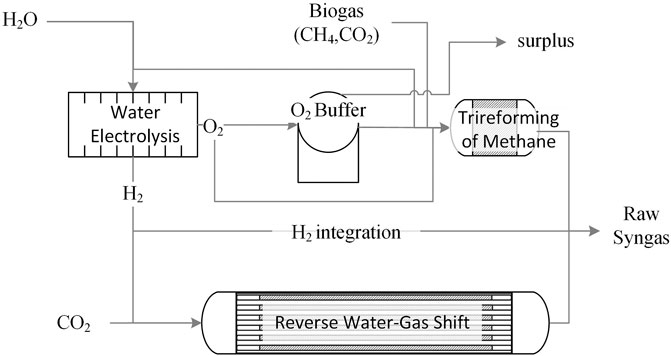
FIGURE 1. Overall Plant layout: the RWGS and TRI reactors produce raw syngas, where H₂ and O₂ are supplied via EL. H₂ may be fed to RWGS and/or bypass the reactor to the syngas product stream whereas excess O₂ may be stored in a buffering device. CO₂ could be obtained from biogas using a suitable separation strategy.

In this framework, the most rational source of CO₂ is biogas, part of which could be split into CH₄ and CO₂via a suitable state-of-the-art separation strategy as reviewed by Maggi et al. (2020), e.g., membranes or PSA. The resulting CH₄ stream would then be used to sustain the heat demand of RWGS. Surplus CH₄ could be injected into the natural gas grid.

3 Mathematical Model

Key modeling assumptions and main governing equations for the reactors are reported in this section. For the sake of clarity, important symbols are introduced within the text, whereas a broader list of symbols is reported in Table 1.

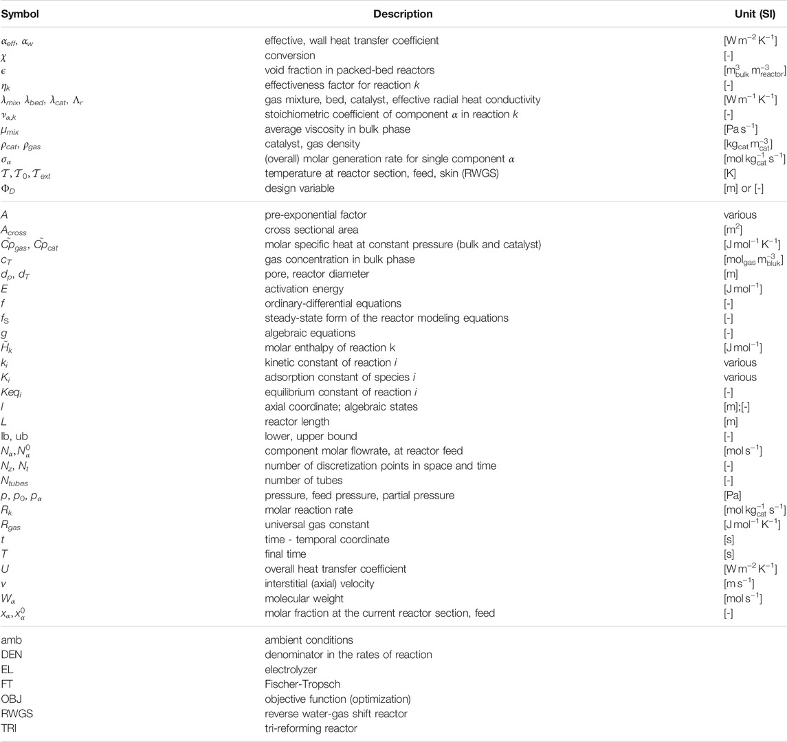
TABLE 1. List of symbols.

3.1 Modeling Assumptions

Prior to the description of the mathematical models, assumptions are here concisely reported. Various assumptions will be elaborated on after the following list.

• Perfect purity and total conversion are associated with EL, for which dynamics are neglected. Therefore, EL is treated as a node, splitting its feed stream into two outlets according to the stoichiometry of water splitting: H₂O → H₂ + 0.5O₂.

• H₂ can be integrated directly from EL into the product stream.

• The difference between O₂ from EL and O₂ to TRI approximates the accumulation of O₂ in the buffering system, which is not directly modeled.

• Biogas is a binary mixture of CH₄ and CO₂ for example provided by anaerobic digestion.

• Feed composition, temperature and pressure at the each reactor feed are fixed, whereas their flowrates can vary.

• RWGS is fed with an equimolar mixture of CO₂ and H₂. The desired feed composition of TRI shall be identified via optimization in Section 4.

• The shell-side temperature at RWGS, denoted as ${\mathcal{T}}_{ext}$, is assumed to be constant along the reactor axis and equal to 1073 K, which is assumed to coincide with the outer skin temperature.

• The electricity demand at EL largely surpasses other contributions, which are therefore neglected in the optimal control application.

The outlets from an electrolyzer will contain traces of unconverted water, which should be removed. In case EL runs at high temperatures, O₂ has to be cooled prior to compression and storage. Consequently, flash condensation constitutes a reasonable option. In addition, H₂O can be removed in steam-selective polymeric membrane separators.

Biogas may contain traces of ammonia and hydrogen sulfide which should be removed before any catalytic operation. These process steps are required. Nevertheless, considering that purification operations would constitute a decoupled optimization problem from the syngas stabilization, i.e., to minimize the concentration of catalyst poisons at their outlets, and considering that the time-scale related to the effects of catalyst deactivation due to poisoning differs from the one related to short-term power fluctuation here investigated, purified biogas is considered in the control volume of the process system analyzed in this study. Furthermore, biogas could vary in its CH₄ concentration, as it may be provided by different biomass feedstock over time, or collected within the plant from different geographical areas in the region. For this reason and for the parametrization of TRI, a lower and upper bound is considered in order to design the plant for the most suitable biogas composition. In case this composition were not perfectly aligned with the actual feed gas, the ratio could be easily adjusted via membrane modules, already implemented to generate a stream of CO₂ intended for RWGS. As a lower bound for the methane concentration in the binary mixture of CO₂ and CH₄ fed to TRI, 55% is selected, whereas 75% is the upper bound, a rather high but possible value, as reported in EBA (2021) and IEA (2021).

The choice of a stoichiometric feed composition at RWGS results from the aim of minimizing the thermal effect that a surplus of H₂ or CO₂ would introduce, as larger gas volumes would be required at the reactor, thus demanding higher heat duty and reactor volume. On the other hand, feeding a molar excess of H₂ would prove reasonable to contain carbon deposition unless the catalyst shows little or no tendency in this direction, which is the case for the rhodium-supported catalyst proposed in this contribution.

The shell-side temperature of RWGS is consistent with the upper threshold of the validation range for the implemented kinetics (873–1073 K). An estimation of the electricity demand for gas compression will be provided with the discussion of results in the following section.

3.2 Modeling of Reactors

This section reports the main governing equations of the reactors as well as further reactor-specific assumptions. Extensive details regarding the modeling of kinetics and heat transfer can be found in the supplementary material – seeSection 7.

Introducing the set of chemical components $\mathcal{S}≔\{{\mathrm{C}\mathrm{O}}_2,{\mathrm{H}}_2,\mathrm{C}\mathrm{O},{\mathrm{H}}_2\mathrm{O},{\mathrm{C}\mathrm{H}}_{\mathrm{4}},{\mathrm{O}}_2\}$, the reactors are described by dynamic, mono-dimensional, pseudo-homogeneous material and energy balances. The material balance for component α in molar formulation reads:

where the molar fraction x_α is differentiated in time and space. Equation 1 has to be fulfilled for all (t, l) ∈ (0, T] × (0, L), where L > 0 specifies the length of the reactor (l is the axial coordinate), T > 0 is the final time (t is the temporal coordinate).

In the energy balance, the temperature $\mathcal{T}$ is differentiated as:

defined for all (t, l) ∈ (0, T] × (0, L), where axial dispersion is neglected. Equation 2 introduces a summation term defined for the relevant kinetics k ∈ K≔ {reverse water-gas shift (RWGS), water-gas shift (WGS), steam-reforming of methane (SR), reverse methantion (RMETH) and catalytic oxidation of methane (OX)}. The term σ_α, concurring to (1), is the overall molar generation rate for the single component α, which reads:

State-of-the-art kinetics reported by Xu and Froment (1989) and De Groote and Froment (1997) are implemented for TRI. Combustion kinetics within TRI were adapted from Trimm and Lam (1980) by De Smet et al. (2001) for supported Ni catalysts. Effectiveness factors for this heterogeneous model are constant and were retrieved from De Groote and Froment (1997). Reversible kinetics of RWGS were taken from Richardson and Paripatyadar (1990), thus based on a Rh/γ −Al₂O₃ catalyst. The effectiveness factor of 0.3 observed by the authors is also incorporated in the calculations for this contribution. For adiabatic operations, i.e., inside the TRI reactor, the overall heat transfer coefficient U is 0, whilst it is U ≠ 0 for the RWGS mildly-endothermic, multitubular reactor.

The axial mole-averaged interstitial velocity v is defined by a total mass balance in quasi-steady state assumption. Mole and mass-averaged velocities coincide if dispersion is neglected. Thus, the molar-based axial velocity defined between the reactor feed (superscript ⁰) and the generic reactor section reads

The momentum balance, typically dominated by friction, reduces to the Ergun equation

The time-dependency of momentum is neglected. Equations 1, 2, and 5 are completed by Dirichlet-type boundary conditions at each reactor inlet, respectively

where x_α,0, ${\mathcal{T}}_0$ and p₀ are the molar fraction of component α, temperature and pressure at the reactor feed, pre-specified and constant over time.

3.3 Semidiscretized Plant Model

After discretizing the reactors by equally-spaced finite volumes in the spatial direction and approximating the advection contributions with the upwind scheme, the resulting system of modeling equations is a semi-explicit differential-algebraic equation (DAE) system of index 1 on the time horizon $\left[0,T\right]$. Thus, it can be written in the form

where $\dot{y}$ is an abbreviation for $\frac{\mathrm{d}y}{\mathrm{d}t}$ and suitable initial values for (7) will be discussed in Section 5. Here:

• $y(t)\in {\mathbb{R}}^d\times [0,T]$ collects all differential variables, i.e., all variables that are differentiated with respect to time. These are the mole fractions coming out of the discretizations inside the RWGS and TRI reactor.

• $z(t)\in {\mathbb{R}}^q\times [0,T]$ collects all algebraic variables. These are the pressure values inside the reactors as well as the outlet molar flowrates from the reactors and the H₂-integration into the plant outlet stream.

• $f:\mathbb{R}\times {\mathbb{R}}^d\times {\mathbb{R}}^q\to {\mathbb{R}}^d$ is a function, collecting all differential equations.

• $g:\mathbb{R}\times {\mathbb{R}}^d\times {\mathbb{R}}^q\to {\mathbb{R}}^q$ is a function, collecting all algebraic equations.

4 Reactor Design

Prior to optimal control, reactor designs for TRI and RWGS are identified separately, ensuring that the desired productivity of 270 ton_CO/day and a syngas ratio of H₂/CO = 2, suitable for Fischer-Tropsch synthesis, are attained in each case.

4.1 Design of TRI

A preliminary optimization problem is set to identify suitable values of the design parameters that maximize the selectivity towards syngas, that is

Here, Equations 1, 2 are implemented in their steady-state formulation such that time derivatives vanish. The resulting modeling equations serve as equality constraints in a nonlinear programming (NLP) problem, that is

where the vector Φ_D collects the optimization variables: tube length L, tube diameter d_T, feed molar flowrates $N_{\alpha }^{in}$ ($\alpha \in \mathcal{S}$), temperature ${\mathcal{T}}_0$ and pressure p₀, and the vector z_S,r which includes all reactor states. The function f_S,r incorporates the conservation laws (1), (2), and (5), where the subscript S indicates the steady-state formulation. Additional constraints bound the syngas composition as ${\mathrm{H}}_2/\mathrm{C}\mathrm{O}\in \left[1.95,2.1\right]$, while the productivity of carbon monoxide is fixed. Problem parameters, constraints and bounds are defined in Matlab v2018b, combined with CasADi v3.5.3, a symbolic framework for algorithmic differentiation and numeric optimization developed by Andersson et al. (2019). The nonlinear program is solved by IPOPT v3.12.3, running with the linear solver mumps, see, e.g., Wächter and Biegler (2006). The solver IPOPT identifies local optima. Therefore, in order to identify a global solution, optimization variables are randomized within bounds. Preliminary simulations in steady-state based on the randomized guesses are then ran in order to provide IPOPT with reasonable initial guesses. Optimal solutions are then compared and the design set ensuring the best objective is selected. The reactor is discretized with 150 equally-spaced points. Optimization variables, bounds and optimal values are reported in Table 2.

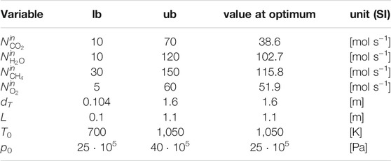
TABLE 2. List of relevant optimization variables for design problems, bounds, and results for TRI.

The selected bounds for the feed pressure to TRI are in line with the findings on the role of coke formation in catalytic partial oxidation of methane by De Groote and Froment (1997) and with the prevailing literature on partial oxidation and tri-reforming. Above 25 bar and for elevated inlet temperatures, coke deposition is neglected.

Moreover, the selected lower bound for the feed pressure at TRI, which coincides with its optimal value reported in Table 2, is consistent with the requirement of a typical Fischer-Tropsch synthesis reactor, i.e., no pressurization is required before this downstream syngas application.

At the best local optimum, the molar selectivity towards H₂ and CO is 2.28. The feed ratio between CH₄ and the sum of CO₂ and CH₄ is 0.75, which corresponds to the upper bound defined for the CH₄ molar content in this binary mixture (seeSection 3.1 for modeling assumptions).

4.2 Design of RWGS

The set of relevant design parameters and operating conditions is reported in Table 3.

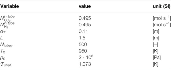
TABLE 3. List of design parameters and nominal operating conditions for RWGS.

Accounting for its drop along the axial coordinate, pressure is slightly above atmospheric, in agreement with the range of validation for the kinetic model by Richardson and Paripatyadar (1990). At the prevailing temperature, pressure and feed composition, the selected feed and shell-side temperature are high enough to prevent from a thermodynamically relevant contribution of the methanation reaction, therefore neglected. The number of discretization points for RWGS simulations and optimal control is 150.

4.3 Steady-State Results

4.3.1 TRI Reactor

Reactor profiles reflect the typical adiabatic operation: non-zero gradients are reported at the beginning, flattening out to zero once the energy input from the catalyzed combustion of CH₄ is exhausted by the endothermic reactions. The selected NLP formulation and objective determine a solution for the reactor length at its upper bound, although the gradients flatten out before its first half. Consequently, the reactor length is reduced by 90% of the upper bound, whereas the value of the remaining optimization variables is set to their optimum. Steady-state simulation profiles are reported in Figure 2: reforming contributions exploit the heat from catalyzed combustion within the very first reactor section. After the adiabatic peak, temperature decreases and stabilizes around 1200 K. The short reactor length determines a negligible pressure drop, in agreement with Chein et al. (2017), and the velocity reflects the temperature profile. Position and magnitude of the high-temperature peak at the very inlet of the reactor is consistent with scenarios presented by Chein et al. (2017), Arab Aboosadi et al. (2011), and Rezaei and Catalan (2020). For the reason that the maximum adiabatic temperature undermines the thermal stability of materials, recommendable studies concerning side-feeding strategies of O₂ by means of membrane and sequential injection points have been proposed by Alipour-Dehkordi and Khademi (2020) and Rezaei and Catalan (2020), although disregarded from the current contribution for sake of mathematical simplicity in the optimal control application. Furthermore, the small ratio between the resulting reactor length and diameter could lead to important radial gradients and an uneven gas distribution, possibly resolved by partitioning the feed stream into a bundle, as proposed by Alipour-Dehkordi and Khademi (2020).

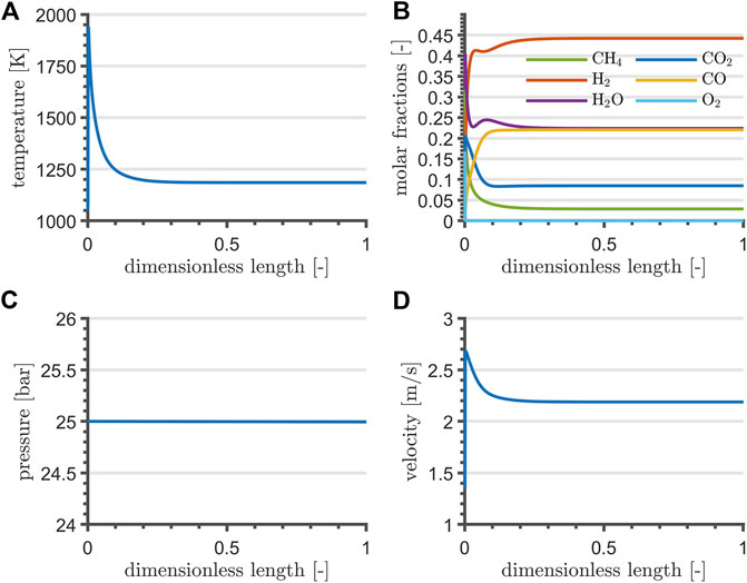
FIGURE 2. TRI temperature (A), composition (B), pressure (C), and velocity profile (D) at steady-state and at nominal flowrate.

Reactor profiles are shown in Figure 3. The temperature profile drops to a minimum within the first quarter of reactor length, where the mass action is at its maximum. Gradually, it shifts towards the shell-side temperature. Temperature and velocity are directly proportional, whereas the pressure drops almost linearly along the reactor length. Simulation results indicate a conversion of 44.7%.

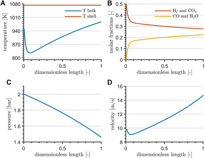
FIGURE 3. RWGS temperature (A), composition (B), pressure (C) and velocity profile (D) at steady-state and at nominal flowrate. For the sake of clarity, (A) reports the shell-temperature of the heating fluid.

Assuming that EL operates at 1073 K, the ideal electrical power demand, which equals the Gibbs free energy of reaction, is 188 kJ${\mathrm{mol}}_{{\mathrm{H}}_{\mathrm{2}}}^{-1}$. Therefore, the nominal flowrate of H₂ to RWGS (247.5 mol_H2s⁻¹) is ensured if EL is supplied with 46.53 MW. Posdziech et al. (2019) identified an EL efficiency of 82%, based on the lower heating-value of H₂ (${\mathrm{L}\mathrm{H}\mathrm{V}}_{{\mathrm{H}}_2}$), corresponding to 240 kJ${\mathrm{mol}}_{{\mathrm{H}}_{\mathrm{2}}}^{-1}$, which outlines a power demand of 72.4 MW. For the given operation, a syngas ratio H₂/CO of 2 is attained if an integration of 85 mol_H2s⁻¹ is accounted for, which corresponds to a total power demand at EL of 62.5 MW, based on the Gibbs free energy, and 97.3 MW, based on the ${\mathrm{L}\mathrm{H}\mathrm{V}}_{{\mathrm{H}}_2}$ efficiency. CH₄ is a candidate fuel to sustain the heat demand of RWGS, possibly provided from biogas. Given that its lower heating value (${\mathrm{L}\mathrm{H}\mathrm{V}}_{{\mathrm{C}\mathrm{H}}_{\mathrm{4}}}$) is 800 kJmol⁻¹, an estimate of the required flowrate is provided by the following calculation, accounting for the reactor discretization (N_z points in axial coordinate and axial discretization segments of length Δz):

resulting in 5.8 mol s⁻¹ of CH₄, 5% of the molar flowrate required for nominal operations of TRI towards the maximum selectivity to syngas (seeTable 2). If biogas has a molar concentration of 60% in CH₄, 9.7 mol s⁻¹ must be separated. Consequently, nominal RWGS operations require considerably less CH₄ than TRI, the latter virtually demanding no electricity other than compression duties.

4.3.3 Oxygen Utilization

Given that the stoichiometric combustion of 5.8 ${\mathrm{m}\mathrm{o}\mathrm{l}}_{{\mathrm{C}\mathrm{H}}_4}$s⁻¹ requires 11.6 ${\mathrm{m}\mathrm{o}\mathrm{l}}_{{\mathrm{O}}_2}$s⁻¹, nominal RWGS operations generate an excess of 155 ${\mathrm{m}\mathrm{o}\mathrm{l}}_{{\mathrm{O}}_2}$s⁻¹ which can be buffered to allow for the operation of TRI in lack of renewable electricity. Assuming that RWGS (TRI is off) and TRI (RWGS is off) are respectively operated for 50% of a given time-horizon, the ratio of O₂ generated (not intended for combustion) to O₂ fed to TRI (Table 2) is 155/52 = 2.98 : 1.98 moles of surplus per mole of oxygen fed to TRI. The stored surplus is possibly further decreased to sustain thermal utility generation within the plant or sold at market value.

5 Optimal Control for the Plant Model

In this section, two different optimal control problems (OCPs) related to the plant model (7) are considered. The control vector $u={(u^{\mathrm{R}\mathrm{W}\mathrm{G}\mathrm{S}},u^{\mathrm{T}\mathrm{R}\mathrm{I}})}^{⊺}\in {\mathbb{R}}^2$ contains the inlet flowrates to the RWGS and TRI reactors, where the feed composition is fixed as assumed in Section 3.1. The inlet molar flowrate to EL, denoted as EL_in, is not treated as a control variable but is pre-defined in the model. Thus, one obtains the H₂-integration to the product stream as

where the composition of u^RWGS, the total inlet flowrate to RWGS, is an equimolar mixture of CO₂ and H₂ as described in Section 3.1. Finally, although the buffer device is not modeled as mentioned in Section 3.1, assuming that O₂ is exclusively intended for the feed to TRI, the accumulation of O₂ inside the buffer can be calculated as

where O_2,TRI,in is the mole fraction of O₂ in the TRI inlet stream and $N_{{\mathrm{O}}_2}^{\mathrm{R}\mathrm{W}\mathrm{G}\mathrm{S},shell}$ is the oxygen required to burn the required amount of methane calculated in (10).

In the first OCP, the control u and the EL inlet flowrate EL_in are constant in time in order to clearly describe the approach. In the second OCP these quantities are then time-dependent functions. As a result, they have to discretized in time such that the amount of control variables scales with the amount of time steps and the problem as a whole becomes more challenging from the optimization point of view.

With the introduced time-constant controls the DAE (7) becomes

Introducing the combined state $w(t)≔{[y(t),z(t)]}^{⊺}\in {\mathbb{R}}^{d+q}$ and the matrix $M≔\left(\begin{array}{cc}\hfill I_{d\times d}\hfill & \hfill 0_{d\times q}\hfill \\ \hfill 0_{q\times d}\hfill & \hfill 0_{q\times q}\hfill \end{array}\right),$ where $I_{d\times d}\in {\mathbb{R}}^{d\times d}$ is the identity matrix, the system can be rewritten as

where the nonlinear function $\tilde{F}:\mathbb{R}\times {\mathbb{R}}^{d+q}\times {\mathbb{R}}^2\to {\mathbb{R}}^{d+q}$ encodes f and g from (13). Based on this formulation, the abstract solution operator$\mathcal{F}:u\mapsto w(t)$ maps a control u to the state solution w(t) of (14). Using this notation, a general OCP in reduced form inlcuding box constraints on the control is proposed as

In this reduced form of the OCP, the state w is not an optimization variable and thus only implicitly known to the optimizer through the solution operator $\mathcal{F}$. As a result, whenever the objective is to be evaluated, the solution operator has to be evaluated for the current value of the control, meaning that (14) has to be solved. Before the numerical solution of (14) is tackled and two specific OCPs are introduced, it is clear that any optimizer applied to (OCP) will require $\frac{\mathrm{d}\mathrm{\Gamma }}{\mathrm{d}u}$, the gradient of the objective function with respect to the control. Thus, the continuous adjoint method from Cao et al. (2003) for its calculation is briefly reviewed.

Introducing a yet unspecified variable $\lambda \in {\mathbb{R}}^{d+q}$, the augmented objective function is formed as

where here and in the following the dependency of $\lambda ,w,\dot{w},F$, and associated quantities on time is often suppressed. Since $F(w,\dot{w},t,u)=0$ due to the reduced approach, the sensitivity of Γ with respect to u is

where the subscripts indicate partial derivatives and the integrals are to be taken component-wise. Integration by parts for the term ${\int }_0^T{\lambda }^{⊺}{F}_{\dot{w}}{\dot{w}}_u\mathrm{d}t$ together with the fact that $F_{\dot{w}}\equiv M$ and further letting the adjoint state$\lambda (t)\in {\mathbb{R}}^{d+q}$ satisfy the adjoint equation

the final sensitivity reads

Thus, the computation of the gradient inside an optimizer requires

• the solution of the forward problem (14),

• the solution of the adjoint problem (17),

• the evaluation of the gradient (18).

Regarding the adjoint Equation 17, which is a linear DAE, it is sufficient to choose initial values such that $\lambda {(T)}^{⊺}M=0$, which is easily obtained according to (Cao et al., 2003, Eq. (9)). Thus, the last term in (18) becomes $\lambda {(0)}^{⊺}M{w}_u(0)$ and one has to calculate w_u(0), the sensitivity of the initial state with respect to the control. The initialization of the system will be covered separately for each OCP after the numerical solution of (14) and (17) is discussed in the following section.

5.1 Numerical Time Integration

Standard Runge-Kutta methods (RKMs) can be adapted to DAEs according to Hairer and Wanner (1996), but the matrix of the tableau has to be invertible such that implicit methods have to be chosen. Thus, a simple implicit Euler scheme is sufficient for the adjoint Equation 17 as it is a linear DAE. Regarding (14), the forward simulation is computationally more demanding, such that parareal is briefly reviewed here, see, e.g., Lions et al. (2001); Baffico et al. (2002); Garmatter et al. (2021), in order to speed up the solution time of the overall OCP.

The main idea of parareal is to decompose the global time domain [0, T] into N_t smaller subdomains. Given initial values on each of these subdomains, the global time-dependent problem in each iteration of the method splits up into N_t many local problems on these subdomains, which can then be solved in parallel. The initial values can be generated using a coarse integrator, which should be cheap but can be inaccurate, and the subproblems are then solved in parallel using a fine integrator, which has to be accurate and is thus more expensive. Afterwards, the next iterate of parareal is generated via a correction step, where the fine solutions of the subproblems are used to correct the coarse sequential integrator.

Introducing the general time grid $0=:t_0<t_1\dots <t_{N_t}≔T$ with variable step sizes h_n≔t_n+1 − t_n, n = 0, …N_t − 1, $\mathfrak{G}(t_{n+1},t_n,h_n,w_n^k)$ denotes the coarse integrator, that integrates on the subdomain [t_n, t_n+1] with step-size h_n and provides an inaccurate approximation to w(t_n+1), the solution of (14), using the initial values $w_n^k$. Here, k indicates the iteration number of parareal. The fine integrator has to be more accurate and can thus be more expensive. This can be achieved by using a higher order integration method or by operating on a refinement of the time grid or a combination of both. In this article, the fine integrator will always be a higher order method and it can additionally operate on a refinement of the time grid such that $\mathfrak{F}(t_{n+1},t_n,R_{\mathrm{r}\mathrm{e}\mathrm{f}},w_n^k)$ denotes the fine integrator, that integrates on [t_n, t_n+1] using $R_{\mathrm{r}\mathrm{e}\mathrm{f}}\in \mathbb{N}$ time steps and provides a more accurate approximation to w(t_n+1) using the initial values $w_n^k$. Thus, for R_ref = 1 both integrators use the same grid and for R_ref ≥ 2 the fine solver $\mathfrak{F}$ uses a refined grid. With this notation at hand, parareal is described in Algorithm 1.

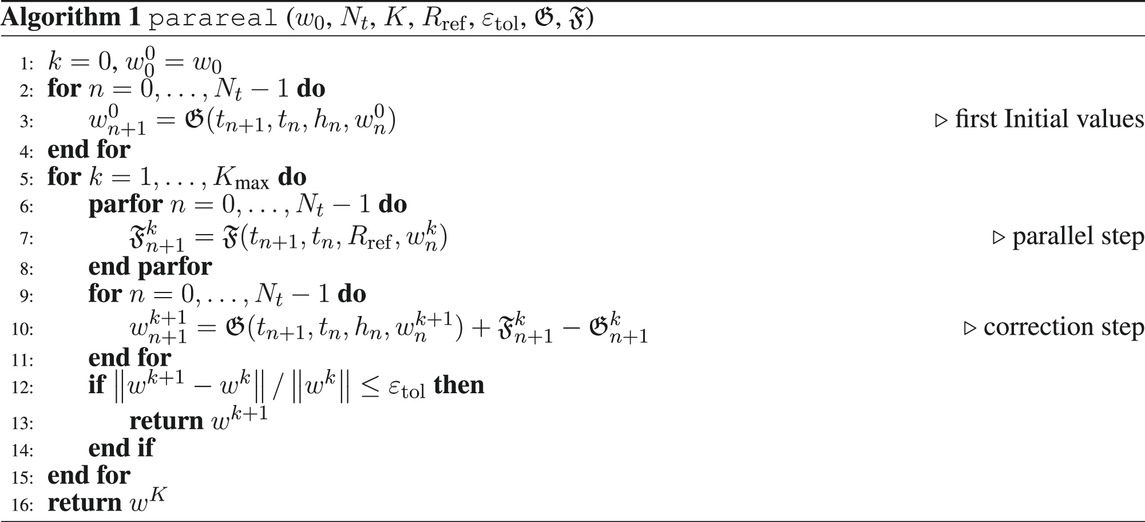
Algorithm 1 is terminated either after a fixed amount of $K_{\text{max}}\in \mathbb{N}$ iterations or as soon as the relative change in the iterate $\left.‖w^{k+1}-w^k\right|/\left.‖w^k\right|$ is below some tolerance ɛ_tol > 0. Note that in line 10, the values of the coarse integrator ${\mathfrak{G}}_{n+1}^k=\mathfrak{G}(t_{n+,1},t_n,h_n,w_n^k)$ have been calculated in the previous iteration already and thus can be reused. Regarding the integrators, $\mathfrak{G}$ should be fast but at the same time an implicit RKM such that the implicit Euler method is chosen and for $\mathfrak{F}$ a higher order method is required such that the Lobatto IIIC method is chosen.

5.2 First OCP

A first optimal control problem based on a tracking-type objective function with an added regularization term is considered. That is, for a given desired state$x_d(t):\mathbb{R}\to {\mathbb{R}}^{d+q}$, the optimal control problem reads

This resembles the scenario: given a desired state x_d(t) and an initial control $u_{\mathrm{i}\mathrm{n}\mathrm{i}\mathrm{t}}\in {\mathbb{R}}^2$, problem (OCP1) wants to find an optimal control $u_{\mathrm{o}\mathrm{p}\mathrm{t}}\in {\mathbb{R}}^2$ for which the corresponding state $\mathcal{F}(u_{\mathrm{o}\mathrm{p}\mathrm{t}})$ best fits the desired state x_d(t). As the desired state will be calculated based on a chosen desired control $u_d\in {\mathbb{R}}^2$, this problem becomes a parameter-identification problem and serves the purpose of validating the mathematical approach rather than resembling an actual application.

Regarding the initialization of the DAE system (14), the initial values $w(0,u)\in {\mathbb{R}}^{d+q}$ are constructed as follows: an intermediate vector ${\tilde{w}}_0\in {\mathbb{R}}^{d+q}$ is formed that consists of fixed values for the mole fractions, the temperature and the pressure at each discretization point inside the reactors. Furthermore, the control u affects the algebraic variables of ${\tilde{w}}_0$ corresponding to the reactor outlet flowrates and the H₂-integration. Next, ${\tilde{w}}_0$ serves as the initial value for a Newton method that solves $\tilde{F}(0,w,u)=0$. The solution of this nonlinear problem then is w(0, u), the actual initial values for the DAE (14) such that these initial values are always consistent. Furthermore, w_u(0) has only nonzero values in the algebraic part, such that Mw_u(0) = 0 and the last term in (18) vanishes.

5.2.1 Numerical Results

Regarding the physical discretization and various model parameters, the same values as in Section 4 are chosen in this section and in the later Section 5.3.1. Furthermore, Matlab v2021a was invoked to obtain these results.

For the solution of (OCP1), Matlab’s fmincon routine with its SQP solver is called, where the objective gradient is calculated via(18), the adjoint state is calculated via(17), and this adjoint equation is solved via the implicit-Euler method. The necessary derivatives of $\tilde{F}$ are calculated via ADiMat, seeBischof et al. (2002). The integrals in (OCP1) and (18) are approximated via the trapezoidal rule. Regarding fmincon, default options and thus default termination criteria are used.

In this academic example, it is T = 1 s and the time horizon [0, 1] is discretized with N_t = 100 equidistant points resulting in $h_0=\cdots =h_{N_t-1}=\frac{1}{N_t}$. For the evaluation of $\mathcal{F}(u)$ during the optimization, either the fine integrator $\mathfrak{F}$ or parareal introduced in Section 5.1 are chosen where parareal is invoked with K_max = 10 and ɛ_tol = 10⁻⁶. Furthermore, viaR_ref = 2, the fine integrator always operates on a refined grid. The computations were carried out on a machine with 60 Intel(R) Xeon(R) CPU E7-4880 v2 @ 2.50 GHz cores, where 50 cores where used for the parallel step.

The experiment consists of solving (OCP1) once using the fine integrator $\mathfrak{F}$ for the evaluations of $\mathcal{F}(u)$ and once using parareal and the achieved speed-up is then of interest. To keep the comparison fair, Matlab is in any case only allowed to use one computational thread inside the RKMs. As discussed in Garmatter et al. (2021), the obtainable speedup using parareal is reduced when using an expensive coarse integrator. To partly lift this downside, the scenario of a cheaper coarse solver is mimicked by selecting 10⁻⁴ as the tolerance for the Newton-solver inside $\mathfrak{G}$ where the tolerance inside $\mathfrak{F}$ is 10⁻⁸.

The remaining experiment setup is (numbers associated to the control u always have the unit of measurement mol.s⁻¹)

• $x_d(t)=\mathcal{F}(u_d)$ with $u_d={(30,1)}^{⊺}$ and EL_in = 30 mol.s⁻¹ is obtained via the coarse solver $\mathfrak{G}$ to prevent inverse crime;

• $u_{\mathrm{i}\mathrm{n}\mathrm{i}\mathrm{t}}={(15,15)}^{⊺}$ simulating a generically active plant;

• $u_l={(0.1,0.1)}^{⊺}$, $u_u={(60,\infty )}^{⊺}$, and β = 10⁻⁶. Here, the upper bound for the RWGS corresponds to two times the inlet flowrate to EL to prevent negative H₂-integration values due to (11).

Regarding the solution quality, the solution of (OCP1) using $\mathfrak{F}$ inside the SQP solver of fmincon was

and the solution using parareal was

Regarding the solution time, the optimization using the fine integrator required 8186 s and the optimization using parareal required 3181 s resulting in a speed-up of 2.57. Here, parareal required on average only one iteration, where it was already discussed in Garmatter et al. (2021) that this quick convergence stems from the used implicit RKM as a coarse solver. The downside of this approach is that parareal on average did spend 70.70 s per iteration in the coarse solver and only 8.73 s in the fine solver. Thus, the obtained speed-up could be improved by using N_t = 100 cores (effectively halving the time spent in the fine solver) but it is clear that the coarse solver does indeed limit the maximum obtainable speed-up. Thus, the use of an implicit explicit (IMEX) numerical scheme, see, e.g., Boscarino (2007); Steiner et al. (2014) for IMEX methods for DAEs, could be investigated to leverage this downside.

5.3 Second OCP

As mentioned in the beginning of Section 5 the control u and the EL inlet flowrate EL_in are now time-dependent. Thus, EL_in is a function of time predefined in the model and a time-dependent control has to be introduced. Remembering the time-grid $0=:t_0<t_1<\dots <t_{N_t}≔T$, the control function is defined to be piecewise constant in time, that is

where the coefficients $u_i\in {\mathbb{R}}^2$ contain the control values on the time interval (t_i−1, t_i]. Together with the control at the initial time point $u(t_0)=u(0)=u_0\in {\mathbb{R}}^2$ and abusing Matlab notation, these coefficients can be collected as

such that the overall control dimension p scales with the number of time steps. The OCP presented in the following shall now capture the scenario described in the Introduction: due to external influences (intermittency of electricity), the inlet flowrate to EL is changing according to a piecewise linear profile and the aim of the OCP then is to stabilize the plant to still yield a desired syngas ratio ${\mathrm{S}\mathrm{R}}_d\in \mathbb{R}$ and flowrate ${\mathrm{S}\mathrm{F}}_d\in \mathbb{R}$ in the product stream of the plant. Letting $\mathrm{S}\mathrm{R}(t):\mathbb{R}\to \mathbb{R}:t\mapsto f_1\left(\right.(\mathcal{F}(u(t)))$ and $\mathrm{S}\mathrm{F}(t):\mathbb{R}\to \mathbb{R}:t\mapsto f_2\left(\right.(\mathcal{F}(u(t)))$ be functions that compute the syngas ratio and flowrate at the outlet at time t, based on the value of the control u(t) and thus the state $\mathcal{F}(u(t))$, the optimal control problem reads

Here, $c_{\mathrm{S}\mathrm{R}}≔\frac{\max \{{\mathrm{S}\mathrm{R}}_d,{\mathrm{S}\mathrm{F}}_d\}}{{\mathrm{S}\mathrm{R}}_d}$ and $c_{\mathrm{S}\mathrm{F}}≔\frac{\max \{{\mathrm{S}\mathrm{R}}_d,{\mathrm{S}\mathrm{F}}_d\}}{{\mathrm{S}\mathrm{F}}_d}$ are scaling constants that ensure that both contributions to the objective function are equally weighted. Furthermore, the dynamic EL inlet flowrate profile is again hard-coded in the model such that it does not appear as a constraint in (OCP2). Together with the dynamic inflow to the RWGS unit (the first control component), the H₂-integration to the syngas outlet stream at each time point can then be determined according to (11).

The initialization of the system (14) for (OCP2) is similar to the initialization described in Section 5.2. The only difference being that the entries of ${\tilde{w}}_0$ corresponding to the mole fractions, the temperature and the pressure inside the reactors come from a steady-state-simulation that reflects the desired syngas ration and flowrate but uses a constant-in-time EL inflow profile. The control values u₀ then again affect the algebraic variables corresponding to the reactor outlet flowrates and the H₂-integration and the resulting ${\tilde{w}}_0$ serves as the initial guess for the Newton method resulting in the consistent initial values.

From a theoretical perspective, it is clear that the formulation in (OCP2) differs from (OCP) due to the time-dependency of the control. Nonetheless, the continuous adjoint method can be applied to calculate the objective gradient, where the necessary details can be found in (Gerdts, 2012, Section 5.3.3).

5.3.1 Numerical Results

A time horizon of 1 h (resulting in T = 3600 s) is chosen to reflect the realistic scenario proposed in (OCP2). As a result, the number of equidistant time-steps in the time-grid is increased to N_t = 200.

Regarding the experiment setup, a steady-state simulation is performed where the control values and the EL inflow are both constant in time for the values of $u={(465,20)}^{⊺}$ and EL = 313 mol.s⁻¹ (numbers associated to the control u again have the unit of measurement mol.s⁻¹). This results in a desired syngas ratio SR_d = 1.9998 and desired syngas flowrate SF_d = 111.44 mol s⁻¹. As mentioned in the previous section, this steady-state simulation is involved in computing the initial values for the DAE system during the optimization. Finally, the EL inflow is now dynamic and the hard-coded flow profile can be seen in the top left of Figure 4.

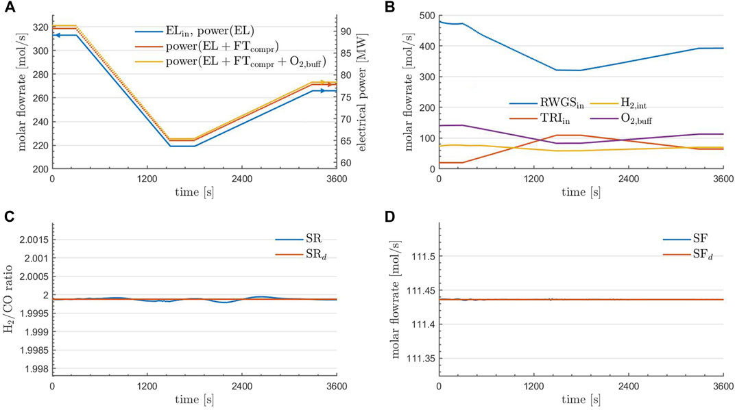
FIGURE 4. Prescribed dynamic inflow to the EL unit of the plant (A). RWGS and TRI inflow as well as H₂-integration and the accumulation of O₂ in the buffering device at optimality (B). Obtained and desired syngas ratio (C), as well as obtained and desired syngas flowrate (D) for the optimal solution using parareal. (A) further contains the cumulative power demands within the control volume based on the calculations reported in Section 5.3.2.

The solution of (OCP2) is carried out as described in Section 5.2.1 and the comparison between the solution using parareal and the solution via the fine integrator $\mathfrak{F}$ is again of interest. The only difference in the solution setup is that fmincon is now also allowed to terminate as soon as the objective function value is below 10⁻³. With sight on the scale of the desired values SF_d and SR_d inside the objective function J₂, this is justified as more precision is not required from an application point of view.

It is the aim of the optimization to adjust the plant activity to still produce the desired syngas ratio and flowrate under this changing inflow to the EL. Finally, the upper and lower bounds u_u(t) and u_l(t) at each time step coincide with the values from Section 5.2.1 with the only difference being that the first value of u_u(t) (the upper bound to the total RWGS inflow) now is two times the value of the EL-profile from the top left of Figure 4 to again prevent negative H₂-integration values. Based on the control values used in the steady state simulation, the initial values for the optimization are constant in time as $u_{\mathrm{i}\mathrm{n}\mathrm{i}\mathrm{t}}(t)={(465,20)}^{⊺}$.

The solutions to (OCP2) are investigated in Figures 4, 5. Here, only the results obtained using parareal are depicted. This is justified, as the results obtained using the fine integrator $\mathfrak{F}$ are qualitatively the same as

Regarding the solution time, the optimization using the fine integrator required 6.56 h and the optimization using parareal required 3.85 h resulting in a speed-up of 1.70. Due to the time-dependent dynamics, parareal now requires on average two iterations although the iteration error in line 12 of Algorithm 1 after the first iteration is on average 2.4956 ⋅ 10⁻⁶ and thus very close to ɛ_tol = 10⁻⁶. The average times spent in the coarse and fine solver per iteration were 233.46 s and 31.16 s. These results are in line with the results from the previous experiment: the coarse/fine time per parareal iteration stems from the increased amount of time steps as well as the second average parareal iteration and the overall increased solution time comes from fmincon requiring more iterations due to (OCP2) being fully time-dependent including the EL profile depicted in the top left of Figure 4. Finally, do note that fmincon was terminated here as soon as the objective function value was lower than 10⁻³ (further note that at termination the first-order optimality was around 1 ⋅ 10⁻³ in both cases). As already mentioned (OCP2) targets a desired syngas flowrate and ratio, such that, due to the scale of the problem, more accuracy for this objective function is not required from an application point of view.

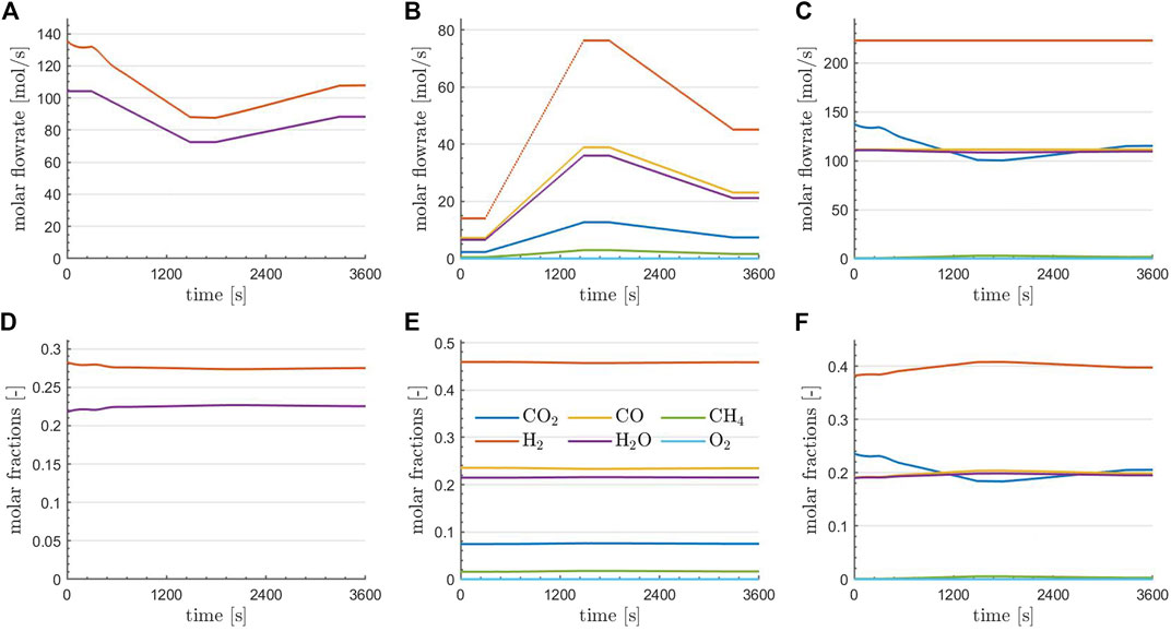
FIGURE 5. Flowrates (A–C) and compositions (D–F) of the various species at the RWGS reactor outlet (A,D), the TRI reactor outlet (B,E), and at the combined plant outlet (C,F) at optimality for the optimal solution obtained using parareal.

Regarding the solution quality, it can be seen in the bottom row of Figure 4 that the aim of the optimization was achieved: the desired syngas ratio and flowrate are matched very well under the prescribed change to the inlet flowrate to EL. In the top right of Figure 4 it can be seen how this was achieved: the inflow to the RWGS unit (blue) is adjusted in accordance to the inflow to EL (top left of Figure 4) and TRI (red) is then activated to still produce the desired amount of syngas. The H₂-integration (yellow) is then a result of (11). Finally, the accumulation rate of O₂ in the buffering device (purple) at each time point can be calculated via(12), where O_2,TRI,in = 0.168 and this value is a result from Table 2.

A more detailed investigation of the optimal state is provided in Figure 5. Here, the flowrates (top row) and flow compositions (bottom row) of the species at the RWGS reactor outlet (left column), the TRI reactor outlet (middle column), and at the combined plant outlet (right column) are depicted. Regarding the reactors, it is observed that the outlet compositions are essentially constant in time, consistent with the fact that equilibrium conditions are essentially met for the given operations. The changes in the outlet flowrates of the reactors are in agreement with the temporal profiles of the controls (the inlet flows to the reactors) depicted in the top right of Figure 4. Finally, it can be observed that an almost complete conversion of CH₄ was achieved and O₂ has entirely been depleted. The flowrate of H₂ and CO is kept constant in time, which was one aim of the optimization. Furthermore, if the content of steam in the raw syngas is constant over time, CO₂ drops at the minimum power input, suggesting that following purification units must handle variable loads of CO₂ over time before feeding the Fischer-Tropsch reactor.

5.3.2 Estimation of the Power Demand for Gas Compression

In Section 3.1 it was assumed that the power demand at EL is the only relevant contribution within the plant. In order to verify this statement, it is assumed that:

• raw substances are fed to the control volume at ambient pressure;

• Fischer-Tropsch (FT) synthesis occurs in a reactor operated at 25 bar;

• the compression work is based on an isothermal transformation at 100°C.

The work demand related to the reactors to attain the pressure level required at the FT reactor, starting from ambient pressure (amb), is estimated as

where it is assumed that process gas flowrates are compressed before TRI, after RWGS and after EL, respectively, $N_{\mathrm{T}\mathrm{R}\mathrm{I}}^0$, $N_{\mathrm{R}\mathrm{W}\mathrm{G}\mathrm{S}}^{out}$ and H_2,int. Similarly, the utility demand for the storage of a molar flowrate O_2,buff oxygen at 300 [bar] is estimated as

The total power demand of the plant is reported in Figure 4A. As it can be seen, the power demand is largely dominated by the electrolyzer, which justifies the assumption made in Section 3.1 related to power consumption in the context of optimal control calculations.

6 Conclusion

A layout for a chemical plant that aims at a syngas production at constant flowrate and a H₂-to-CO-ratio of 2 suitable for Fischer-Tropsch synthesis from renewable power, H₂O and biogas was presented. The plant included a reverse water-gas shift (RWGS) reactor, which was to be used unless power shortage prevented the operation of the electrolyzer and thus the H₂ supply for the RWGS unit. A tri-reforming reactor was thus included into the plant to still provide the desired syngas flowrate and ratio at the product stream. An optimal control problem set to ensure a desired syngas ratio and flowrate at the plant outlet over a prescribed time horizon, given a variable power provision to the electrolyzer, was presented. From the mathematical side, parareal was utilized to speed up the expensive forward time integrations during the optimization and the continuous adjoint method was employed to compute the derivatives of the objective function. In a numerical investigation this novel approach was compared to the scenario where a traditional Runge-Kutta-Method was used for the time integration. It could be seen that both methods yielded qualitatively the same optimal solution, while the novel approach was significantly faster due to parareal. Furthermore, the objective of the optimal control problem was achieved: the desired syngas flowrate and ratio were matched over time under a prescribed piecewise linear inflow profile to the electrolyzer.

From an engineering perspective, the numerical results allowed to identify appropriate feeding strategies at the reactors responding to a fluctuation in power supply and to monitor the temporal composition in the outlet stream and the accumulation of oxygen in the buffering device.

Future research paths should set the proposed layout in the framework of a thorough cost-based technological comparison with alternative buffering strategies for renewable power to syngas (buffering of H₂). Besides, appropriate O₂-dosing strategies to decrease the temperature levels at tri-reforming should be accounted for, as well as a suitable strategy for the buffering of oxygen. The inclusion of heat exchangers and compressors would surely set feasibility bounds to the flexibility of the plant, an important aspect to be addressed. From a process-control perspective, it would be desirable to relax the condition of fixed temperature, pressure and composition at the reactors inlets throughout the control horizon. Furthermore, a mathematical investigation regarding the coarse solver inside parareal should be accounted for. Here, a faster solver could provide even more speed-up for the overall approach. As a result, a more in-depth analysis of the engineering model or even a real-time application could then become possible.

7 Supplementary Material

In this section, modeling details and parametrization is reported.

7.1 Reaction Rates for Tri-reforming of Methane

The parameters are selected from Xu and Froment (1989) and reported in Table 4. The governing kinetic expressions are

• $\mathrm{D}\mathrm{E}\mathrm{N}=\left(1+K_{\mathrm{C}\mathrm{O}}{p}_{\mathrm{C}\mathrm{O},[bar]}+K_{{\mathrm{H}}_2}{p}_{{\mathrm{H}}_2,[bar]}+K_{{\mathrm{C}\mathrm{H}}_{\mathrm{4}}}{p}_{{\mathrm{C}\mathrm{H}}_{\mathrm{4}},[bar]}+K_{{\mathrm{H}}_2\mathrm{O}}\frac{x_{{\mathrm{H}}_2\mathrm{O}}}{x_{{\mathrm{H}}_2}}\right)$,

• $R_{SR}=10^3\frac{k_{SR}}{p_{{\mathrm{H}}_2,[bar]}^{2.5}}\left(p_{{\mathrm{C}\mathrm{H}}_{\mathrm{4}},[bar]}{p}_{{\mathrm{H}}_2\mathrm{O},}-p_{{\mathrm{H}}_2,[bar]}^3\frac{p_{\mathrm{C}\mathrm{O},[bar]}}{Ke{q}_{SR}}\right)/DE{N}^2$,

• $R_{WGS}=10^3\frac{k_{WGS}}{p_{{\mathrm{H}}_2,[bar]}}\left(p_{\mathrm{C}\mathrm{O},[bar]}{p}_{{\mathrm{H}}_2\mathrm{O},[bar]}-p_{{\mathrm{H}}_2,[bar]}\frac{p_{{\mathrm{C}\mathrm{O}}_2,[bar]}}{Ke{q}_{WGS}}\right)/DE{N}^2$,

• $R_{RMETH}=10^3\frac{k_{RMETH}}{p_{{\mathrm{H}}_2,[bar]}^{3.5}}\left(p_{{\mathrm{C}\mathrm{H}}_{\mathrm{4}},[bar]}{p}_{{\mathrm{H}}_2\mathrm{O},[bar]}^2-p_{{\mathrm{H}}_2,[bar]}^4\frac{p_{{\mathrm{C}\mathrm{O}}_2,[bar]}}{Ke{q}_{RMETH}}\right)/DE{N}^2$,

• $R_{COMB}=\frac{k_{a,COMB}{p}_{{\mathrm{C}\mathrm{H}}_{\mathrm{4}},[bar]}{p}_{{\mathrm{O}}_2,[bar]}}{{\left(1+K_{{\mathrm{C}\mathrm{H}}_{\mathrm{4}},COMB}{p}_{{\mathrm{C}\mathrm{H}}_{\mathrm{4}},[bar]}+K_{{\mathrm{O}}_2,COMB}{p}_{{\mathrm{O}}_2,[bar]}\right)}^2}+\frac{k_{b,COMB}{p}_{{\mathrm{C}\mathrm{H}}_{\mathrm{4}},[bar]}{p}_{{\mathrm{O}}_2,[bar]}}{\left(1+K_{{\mathrm{C}\mathrm{H}}_{\mathrm{4}},COMB}{p}_{{\mathrm{C}\mathrm{H}}_{\mathrm{4}},[bar]}+K_{{\mathrm{O}}_2,COMB}{p}_{{\mathrm{O}}_2,[bar]}\right)}$,

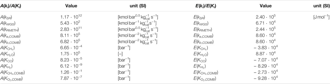
TABLE 4. List of parameters for TRI kinetics: pre-exponential and activation energies.

where the kinetics parameters k_i and K_j related to reaction and adsorption result from the following Arrhenius-like relations

$k_i=A(k_i)\exp \left(-\frac{E(k_i)}{R_{gas}\mathcal{T}}\right)\mathrm{a}\mathrm{n}\mathrm{d}{K}_j=A(K_j)\exp \left(-\frac{E(K_j)}{R_{gas}\mathcal{T}}\right).$(23)

Values of coefficients A(k_i, K_j) and E(k_i, K_j) are listed in Table 4.

7.2 Reaction Rates for RWGS

RWGS kinetics are adapted from Richardson and Paripatyadar (1990).

$\mathrm{D}\mathrm{E}\mathrm{N}=\left(1+K_{{\mathrm{C}\mathrm{O}}_2}{p}_{{\mathrm{C}\mathrm{O}}_2,[\mathrm{a}\mathrm{t}\mathrm{m}]}+K_{{\mathrm{H}}_2}{p}_{{\mathrm{H}}_2,[\mathrm{a}\mathrm{t}\mathrm{m}]}\right)$(24)

and

$R_{\mathrm{R}\mathrm{W}\mathrm{G}\mathrm{S}}=10^3{k}_{\mathrm{R}\mathrm{W}\mathrm{G}\mathrm{S}}{K}_{{\mathrm{C}\mathrm{O}}_2}{K}_{{\mathrm{H}}_2}\left(p_{{\mathrm{C}\mathrm{O}}_2,[\mathrm{a}\mathrm{t}\mathrm{m}]}{p}_{{\mathrm{H}}_2,[\mathrm{a}\mathrm{t}\mathrm{m}]}-\frac{p_{\mathrm{C}\mathrm{O},[\mathrm{a}\mathrm{t}\mathrm{m}]}{p}_{{\mathrm{H}}_2\mathrm{O},[\mathrm{a}\mathrm{t}\mathrm{m}]}}{Ke{q}_{\mathrm{R}\mathrm{W}\mathrm{G}\mathrm{S}}}\right)/{\mathrm{D}\mathrm{E}\mathrm{N}}^2,$(25)

Where kinetics parameters k_i and K_j related to reaction and adsorption, result from Arrhenius-like relations

$k_{RWGS}=350\exp \left(\frac{-81030}{R_{gas}\mathcal{T}}\right),K_{{\mathrm{C}\mathrm{O}}_2}=0.5771\exp \left(\frac{9262}{R_{gas}\mathcal{T}}\right),K_{{\mathrm{H}}_2}=1.494\exp \left(\frac{6025}{R_{gas}\mathcal{T}}\right).$(26)

Effectiveness factor is set to 0.3, as reported in Richardson and Paripatyadar (1990).

7.3 Overall Heat Transfer Coefficient RWGS

The overall heat transfer coefficient reads

$U={\left(\frac{1}{{\alpha }_{eff}}\right)}^{-1}.$(27)

The shell-side heat transfer coefficient is not accounted for. Instead, a constant skin temperature is assumed along the pipe. The definition of α_eff for non-adiabatic packed-bed reactors is provided by Martin and Nilles (1993).

$\frac{1}{{\alpha }_{eff}}=\left(\frac{1}{{\alpha }_w}+\frac{d_T}{8{\mathrm{\Lambda }}_r}\right).$(28)

Here, α_w and Λ_r are retrieved from Bauer and Schlünder (1976) and discussed by Tsotsas (2010) as well as Martin and Nilles (1993).

${\alpha }_w=\left[\left(1.3+\frac{5}{d_T/d_p}\right)\frac{{\lambda }_{bed}}{{\lambda }_{mix}}+0.19{\left[{\rho }_{gas}vϵ\frac{d_P}{{\mu }_{mix}}\right]}^{0.75}{\left[{\mu }_{mix}\frac{{\widetilde{Cp}}_{gas}}{{\lambda }_{mix}}\right]}^{0.33}\right]\frac{{\lambda }_{mix}}{d_p}$(29)

and

${\mathrm{\Lambda }}_r=\left[{\lambda }_{bed}+\frac{vϵc_T{\widetilde{Cp}}_{gas}{d}_p}{8\left[2-{\left(1-\frac{2}{d_T/d_p}\right)}^2\right]}\right].$(30)

Embedded in the definition of α_w, the heat conductivity across the packed-bed λ_bed is defined in Tsotsas (2010) by the following steps:

• λ_bed = k_bedλ_mix,

• $k_{bed}=\left(1-\sqrt{1-ϵ}\right)ϵ\left[{\left(ϵ-1+\frac{1}{k_G}\right)}^{-1}+k_{rad}\right]+\sqrt{1-ϵ}\left(\varphi k_p+\left(1-\varphi \right)k_C\right)$,

• ϕ = 0.0077 [−] spheres,

• $k_C=\frac{2}{N}\left(\frac{B\left(k_p+k_{rad}-1\right)}{N^2\cdot k_G\cdot k_P}\log \left(\frac{k_p+k_{rad}}{B\left(k_G+\left(1-k_G\right)\cdot \left(k_P+k_{rad}\right)\right)}\right)\right.\left.+\frac{B+1}{2B}\left(\frac{k_{rad}}{k_G}-B\left(1+\frac{1-k_G}{k_G}{k}_{rad}\right)\right)-\frac{B-1}{N\cdot k_G}\right)$

• $k_{rad}=\frac{4{\sigma }_{SB}}{2/{ϵ}_E-1}{\mathcal{T}}^3\frac{d_p}{{\lambda }_{mix}}$, σ_SB = 5.67 ⋅ 10⁻⁸ [Wm⁻²K⁻⁴], ϵ_E = 0.4 [−], k_G = 1 [−],

• $B=1.25{\left(\frac{1-ϵ}{ϵ}\right)}^{(10/9)},\text{and}{k}_p=\frac{{\lambda }_{cat}}{{\lambda }_{mix}}$.

Data Availability Statement

The raw data supporting the conclusions of this article will be made available by the authors, without undue reservation.

Author Contributions

AM contributed Sections 2, 3, 4, and 7: he provided the plant layout, the governing equations as well as the corresponding kinetics and the optimal parameters for the different reactors. DG contributed Section 5: he implemented the optimal control approach as well as parareal, developed the combination of the continuous adjoint method and parareal and provided the main numerical results. AM is supervised by KS, DG is mentored by MS. SS aided in the optimal control approach.

Funding

DG, SS, and MS acknowledge the financial support by the Federal Ministry of Education and Research of Germany with in the project P2Chem (support code 05M18OCB).

Conflict of Interest

The authors declare that the research was conducted in the absence of any commercial or financial relationships that could be construed as a potential conflict of interest.

Publisher’s Note

All claims expressed in this article are solely those of the authors and do not necessarily represent those of their affiliated organizations, or those of the publisher, the editors and the reviewers. Any product that may be evaluated in this article, or claim that may be made by its manufacturer, is not guaranteed or endorsed by the publisher.

Acknowledgments

DG acknowleges the vital discussions regarding the continuous adjoint method provided by Prof. Matthias Gerdts.

References

Alipour-Dehkordi, A., and Khademi, M. H. (2020). O2, H2O or CO2 Side-Feeding Policy in Methane Tri-reforming Reactor: The Role of Influencing Parameters. Int. J. Hydrogen Energ. 45, 15239–15253. doi:10.1016/j.ijhydene.2020.03.239
Andersson, J. A. E., Gillis, J., Horn, G., Rawlings, J. B., and Diehl, M. (2019). CasADi: A Software Framework for Nonlinear Optimization and Optimal Control. Math. Prog. Comp. 11, 1–36. doi:10.1007/s12532-018-0139-4
Arab Aboosadi, Z., Jahanmiri, A. H., and Rahimpour, M. R. (2011). Optimization of Tri-reformer Reactor to Produce Synthesis Gas for Methanol Production Using Differential Evolution (DE) Method. Appl. Energ. 88, 2691–2701. doi:10.1016/j.apenergy.2011.02.017
Baffico, L., Bernard, S., Maday, Y., Turinici, G., and Zérah, G. (2002). Parallel-in-time Molecular-Dynamics Simulations. Phys. Rev. E 66, 057701. doi:10.1103/PhysRevE.66.057701
Bauer, R., and Schlünder, E. U. (1976). Effektive radiale Wärmeleitfähigkeit gasdurchströmter Schüttungen aus Partikeln unterschiedlicher Form. Chem. Ingenieur Technik 48, 227–228. doi:10.1002/cite.330480309
Bischof, C. H., Bücker, H. M., Lang, B., Rasch, A., and Vehreschild, A. (2002). “Combining Source Transformation and Operator Overloading Techniques to Compute Derivatives for MATLAB Programs,” in Proceedings of the Second IEEE International Workshop on Source Code Analysis and Manipulation (SCAM 2002), Montreal, QC, Canada, October 1, 2002 (IEEE Computer Society), 65–72. doi:10.1109/SCAM.2002.1134106
Boscarino, S. (2007). Error Analysis of IMEX Runge-Kutta Methods Derived from Differential-Algebraic Systems. SIAM J. Numer. Anal. 45, 1600–1621. doi:10.1137/060656929
Cao, Y., Li, S., and Petzold, L. (2002). Adjoint Sensitivity Analysis for Differential-Algebraic Equations: Algorithms and Software. J. Comput. Appl. Math. 149, 171–191. doi:10.1016/s0377-0427(02)00528-9
Cao, Y., Li, S., Petzold, L., and Serban, R. (2003). Adjoint Sensitivity Analysis for Differential-Algebraic Equations: The Adjoint DAE System and its Numerical Solution. SIAM J. Sci. Comput. 24, 1076–1089. doi:10.1137/s1064827501380630
Chein, R.-Y., Wang, C.-Y., and Yu, C.-T. (2017). Parametric Study on Catalytic Tri-reforming of Methane for Syngas Production. Energy 118, 1–17. doi:10.1016/j.energy.2016.11.147
Daza, Y. A., and Kuhn, J. N. (2016). CO2conversion by Reverse Water Gas Shift Catalysis: Comparison of Catalysts, Mechanisms and Their Consequences for CO2conversion to Liquid Fuels. RSC Adv. 6, 49675–49691. doi:10.1039/c6ra05414e
De Groote, A. M., and Froment, G. F. (1997). The Role of Coke Formation in Catalytic Partial Oxidation for Synthesis Gas Production. Catal. Today 37, 309–329. doi:10.1016/s0920-5861(97)00013-8
De Smet, C. R. H., De Croon, M. H. J. M., Berger, R. J., Marin, G. B., and Schouten, J. C. (2001). Design of Adiabatic Fixed-Bed Reactors for the Partial Oxidation of Methane to Synthesis Gas. Application to Production of Methanol and Hydrogen-For-Fuel-Cells. Chem. Eng. Sci. 56, 4849–4861. doi:10.1016/s0009-2509(01)00130-0
EBA (2021). About Biogas and Biomethane. Available at: https://www.europeanbiogas.eu/about-biogas-and-biomethane (Accessed June 30, 2021).
Engeland, K., Borga, M., Creutin, J.-D., François, B., Ramos, M.-H., and Vidal, J.-P. (2017). Space-time Variability of Climate Variables and Intermittent Renewable Electricity Production - A Review. Renew. Sust. Energ. Rev. 79, 600–617. doi:10.1016/j.rser.2017.05.046
Garmatter, D., Maggi, A., Wenzel, M., Monem, S., Hahn, M., Stoll, M., et al. (2021). “Power-to-chemicals: A Superstructure Problem for Sustainable Syngas Production,” in Mathematical Modeling, Simulation and Optimization for Power Engineering and Management. Editors S. Göttlich, M. Herty, and A. Milde (Berlin: Springer), 145–168. doi:10.1007/978-3-030-62732-4_7
Hairer, E., and Wanner, G. (1996). Solving Ordinary Differential Equations II. Berlin: Springer. doi:10.1007/978-3-642-05221-7
IEA (2021). Report Extract: an Introduction to Biogas and Biomethane. Available at: https://www.iea.org/reports/outlook-for-biogas-and-biomethane-prospects-for-organic-growth/an-introduction-to-biogas-and-biomethane (Accessed June 30, 2021).
Kaiser, P., Unde, R. B., Kern, C., and Jess, A. (2013). Production of Liquid Hydrocarbons with CO2as Carbon Source Based on Reverse Water-Gas Shift and Fischer-Tropsch Synthesis. Chem. Ingenieur Technik 85, 489–499. doi:10.1002/cite.201200179
Lions, J.-L., Maday, Y., and Turinici, G. (2001). Résolution d'EDP par un schéma en temps "pararéel ». Comptes Rendus de l'Académie des Sci. - Ser. - Math. 332, 661–668. doi:10.1016/S0764-4442(00)01793-6
Maggi, A., Wenzel, M., and Sundmacher, K. (2020). Mixed-integer Linear Programming (MILP) Approach for the Synthesis of Efficient Power-To-Syngas Processes. Front. Energ. Res. 8, 161. doi:10.3389/fenrg.2020.00161
Martin, H., and Nilles, M. (1993). Radiale Wärmeleitung in Durchströmten Schüttungsrohren. Chem. Ingenieur Technik 65, 1468–1477. doi:10.1002/cite.330651206
Posdziech, O., Schwarze, K., and Brabandt, J. (2019). Efficient Hydrogen Production for Industry and Electricity Storage via High-Temperature Electrolysis. Int. J. Hydrogen Energ. 44, 19089–19101. doi:10.1016/j.ijhydene.2018.05.169
Rezaei, E., and Catalan, L. J. J. (2020). Evaluation of CO2 Utilization for Methanol Production via Tri-reforming of Methane. J. CO2 Utilization 42, 101272. doi:10.1016/j.jcou.2020.101272
Richardson, J. T., and Paripatyadar, S. A. (1990). Carbon Dioxide Reforming of Methane with Supported Rhodium. Appl. Catal. 61, 293–309. doi:10.1016/s0166-9834(00)82152-1
Schill, W.-P. (2014). Residual Load, Renewable Surplus Generation and Storage Requirements in Germany. Energy Policy 73, 65–79. doi:10.1016/j.enpol.2014.05.032
Sinn, H.-W. (2017). Buffering Volatility: A Study on the Limits of Germany's Energy Revolution. Eur. Econ. Rev. 99, 130–150. doi:10.1016/j.euroecorev.2017.05.007
Song, C., and Pan, W. (2004). Tri-reforming of Methane: A Novel Concept for Catalytic Production of Industrially Useful Synthesis Gas with Desired H2/CO Ratios. Catal. Today 98, 463–484. doi:10.1016/j.cattod.2004.09.054
Steiner, J., Ruprecht, D., Speck, R., and Krause, R. (2014). “Convergence of Parareal for the Navier-Stokes Equations Depending on the Reynolds Number,” in Numerical Mathematics and Advanced Applications - ENUMATH 2013. Lecture Notes in Computational Science and Engineering. Editors A. Abdulle, S. Deparis, D. Kressner, F. Nobile, and M. Picasso (Cham: Springer) 103, 195–202. doi:10.1007/978-3-319-10705-9_19
Trimm, D. L., and Lam, C.-W. (1980). The Combustion of Methane on Platinum-Alumina Fibre Catalysts-I. Chem. Eng. Sci. 35, 1405–1413. doi:10.1016/0009-2509(80)85134-7
Tsotsas, E. (2010). “M7 Heat and Mass Transfer in Packed Beds with Fluid Flow,” in VDI Heat Atlas. Editor VDI-Gesellschaft Verfahrenstechnik und Chemieingenieurwesen (Berlin, Heidelberg: Springer Berlin Heidelberg), 1327–1342. doi:10.1007/978-3-540-77877-6_100
Vita, A., Italiano, C., Previtali, D., Fabiano, C., Palella, A., Freni, F., et al. (2018). Methanol Synthesis from Biogas: A Thermodynamic Analysis. Renew. Energ. 118, 673–684. doi:10.1016/j.renene.2017.11.029
Wächter, A., and Biegler, L. T. (2006). On the Implementation of an interior-point Filter Line-Search Algorithm for Large-Scale Nonlinear Programming. Math. Program 106, 25–57. doi:10.1007/s10107-004-0559-y
Wulf, C., Zapp, P., and Schreiber, A. (2020). Review of Power-To-X Demonstration Projects in Europe. Front. Energ. Res. 8, 191. doi:10.3389/fenrg.2020.00191
Keywords: syngas, reforming, reverse water-gas shift, renewable hydrogen, dynamic optimal control, adjoint method, parallel in time
Citation: Maggi A, Garmatter D, Sager S, Stoll M and Sundmacher K (2021) Power-to-Syngas: A Parareal Optimal Control Approach. Front. Energy Res. 9:720489. doi: 10.3389/fenrg.2021.720489
Received: 04 June 2021; Accepted: 16 July 2021;
Published: 16 September 2021.
Edited by:
Grazia Leonzio, Imperial College London, United KingdomReviewed by:
Mariano Martín, University of Salamanca, SpainBorja Hernández, University of Salamanca, Spain
Copyright © 2021 Maggi, Garmatter, Sager, Stoll and Sundmacher. This is an open-access article distributed under the terms of the Creative Commons Attribution License (CC BY). The use, distribution or reproduction in other forums is permitted, provided the original author(s) and the copyright owner(s) are credited and that the original publication in this journal is cited, in accordance with accepted academic practice. No use, distribution or reproduction is permitted which does not comply with these terms.
*Correspondence: Andrea Maggi, maggi@mpi-magdeburg.mpg.de; Dominik Garmatter, dominik.garmatter@mathematik.tu-chemnitz.de
†These authors have contributed equally to this work and share first authorship