A novel data-driven multi-energy load forecasting model

Introduction

Energy has always played a fundamental role in modern society and economy, and has shown great importance in the past three industrial technological revolutions. The ongoing fourth technological revolution will be no exception, and revolutionary breakthroughs in the energy sector are bound to become the focus (Liu et al., 2020; Chen et al., 2021). Promoting the strategies of carbon peaking and carbon neutrality is a broad and profound transformation of social and economic systems, in which the low-carbon transformation of the energy system will be the key to achieving the “dual carbon” goal. In order to ensure the realization of the “dual carbon” goal, high-proportion renewable energy related supporting technologies should be strengthened, especially the planning and operation of IES (Liu et al., 2021). In the planning and operation of the IES, it is necessary to accurately forecast the multi-energy loads, that is, predicting the future energy demands according to the historical load data, and the available resources, such as wind, solar, electricity, heat, etc.; then, the optimal planning and design or operation scheduling scheme can be determined (Liu et al., 2019). Accurate energy forecasting requires attention to the type, size and operation characteristics of energy demand. The IES often involves a variety of energy forms such as electricity, gas, cooling, and heat, which will always affect each other. This requires for a series of data mining and analysis in the pre-design stage.

Up to present, plenty of researches have been conducted on models and algorithms for the electric load forecasting. Vanting et al. (2021) investigated state-of-the-art electric load forecasting models using deep neural networks from two main perspectives: demand-side management and supply-side grid control. Each perspective had multiple applications and challenges in achieving accurate predictions, including households, buildings, and power grids. Other studies, such as, Liao et al. (2022) proposed a novel decomposition-based ensemble model for short-term load forecasting using hybrid artificial neural networks. (Rochareis and Alvesdasilva, 2005) proposed a feature extraction method for short-term load forecasting through multiresolution analysis. Zhang et al. (2019) presented an integrated load forecasting model for multi-energy systems based on Markov chain improved neural network. Sun et al. (2017) proposed a short-term load forecasting model based on multi-label technology and Back Propagation Neural Networks (BPNN). However, most of the existing load forecasting methods have not considered the coupling effect between multiple energy sources, which is not able to satisfy the optimal planning and operation of the integrated energy systems.

Some other studies have been focused on the optimal operation of power systems or integrated energy systems, using the load forecasts as input data, i.e., Guo, et al., studied multi-objective optimization methods for a distributed energy system, using the community-scale load forecasting data (Guo et al., 2022). Song et al. (2019) proposed a hybrid forecasting system based on multi-objective optimization for short-term electricity load prediction. (Yang and Wang, 2021) studied the optimal operation of an integrated energy system, considering the multi energy coupling effect. It can be seen from the literature review that high-precision load forecasting under the coupling of multiple energy sources is the basis for optimal planning and operation. However, only very limited references have taken account of the coupling effect of multiple energy sources, i.e., Zhang et al. (2021) proposed a short-term multi-energy load forecasting method based on CNN-Seq2Seq model with attention mechanism. Wang et al. (2020; 2021) presented a multi-energy load forecasting method for regional integrated energy systems, considering the temporal dynamics and various coupling characteristics. Compared with traditional electric load forecasting, there are more load types and the loads are more sensitive to various influencing factors, such as the coupling effect between loads and strong environmental uncertainty, which makes the load fluctuation of IES more complex and changeable.

In order to deal with the strong coupling and high uncertainty issues in IES, a novel data-driven multi-energy load forecasting model is proposed in this paper. The main innovative work and contributions of this paper are as follows:

1) A feature dimensionality reduction method of input data for multi-energy load forecasting of the IES based on UMAP is proposed, which realizes the effective selection of complex high-dimensional nonlinear data.

2) A multi-energy load forecasting model based on TCN-NBeats model fusion considering multi-energy coupling correlation is established, which significantly improves the multi-energy load prediction accuracy.

3) The real historical data of multi-energy in different seasons are used to verify the superiority and generalization ability of the feature dimension reduction method and multi-energy load prediction model proposed in this paper.

Feature extraction based on UMAP

For the data-driven multi-energy load forecasting problem, the input features usually include related variables such as meteorological forecast, historical load information, etc., which leads to a large input dimension of the load forecasting model, and it is difficult to extract the relevant information between the features and the forecast output (Liu et al., 2015). Traditional feature map dimensionality reduction methods such as Principal Component Analysis (PCA) can only construct linear representations of input variables, which have great limitations when applied to complex high-dimensional nonlinear datasets. In fact, for the meteorological, historical load and other data, the actual probability distribution does not always fill the entire high-dimensional space, but only concentrates in a part of the region under the action of data correlation, which is called a manifold. In this regard, UMAP starts from preserving the local distance of the adjacent sample points, and maps the sample points on the high-dimensional manifold space to the low-dimensional Euclidean space.

UMAP believes that the local space on the Riemannian manifold is homeomorphic to the Euclidean space, that is, it still has the properties of the Euclidean space, and the sample difference in the local space can still be measured by the Euclidean distance. On this basis, UMAP feature dimensionality reduction can be divided into two main steps:

1) Construct the neighboring connection graph of each sample, that is, obtain the local connection relationship and distance between each sample.

Given an input sample set $X=\{x_1,x_2,\mathrm{...},x_N\}$, define the distance metric between any two sample points as $d:X\times X\to R\ge 0$. Under this metric space, the set of $k$ neighboring samples of the sample $x_i$ can be expressed as $\{x_{i_1},x_{i_2},\mathrm{...},x_{i_k}\}$, then the weights of the edges in the weighted directed graph composed of the sample and its neighboring samples can be calculated as:

Where: ${\rho }_i=min\left\{d(x_i,x_{i_j})\right|1\le j\le k\}$, ${\sigma }_i$ satisfies ${\displaystyle \sum }_{j=1}^{k}w(x_i,x_{i_j})={\log }_2\left(k\right)$. On the basis of this weight definition, a weighted directed graph $G=\left(X,E,w\right)$ of the sample set $X$ can be constructed through nearest neighbor search algorithms such as Neural Network Descent (Teng and Li, 2015), where $E$ is a set composed of directed edges between samples defined by the weight coefficient $w$. The weight $w(x_i,x_{i_j})$ can be understood as the probability that the one-way edge exists. Considering the calculation of the probability of the existence of a bidirectional edge under the above definition, the calculation of the bilateral probability may be different. UMAP makes the following transformation on the existence probability $w_{il}$ of edge $(x_i,x_l)$:

Where: $W$ is the weighted adjacency matrix of the graph $G$; $\circ$ is the Hadamard product of the matrix; and $W\prime$ is the transformed edge weight matrix.

2) Map the neighboring graph to a low-dimensional space while preserving the information of the neighboring graph as much as possible.

Given the input sample set $X$, we need to obtain its sample representation $Y$ in the low-dimensional space, and keep the graph $G$ defined by $X$ and the edge weight matrix $W\prime$ unchanged, that is, the probability weight $w{\prime }_{ij}$ between any sample $x_i$ and its adjacent samples $x_{i_j}$ remains unchanged. UMAP uses the cross-entropy as the loss function to express the difference of the adjacency weight distribution of a single sample, namely:

Where: $v{\prime }_{ik}$ is the probability weight between the sample $y_i$ and the adjacent sample $y_{i_j}$ in the low-dimensional space, which satisfies:

Where: $min\_dist$ denotes the expected interval between closed points in an embedded space.

The mapping construction problem of the sample set $X$ can be transformed into an optimization problem of minimizing the cross-entropy. Since $\mathrm{w}{\prime }_{ik}$ is also a fixed value for a given $X$, the optimization problem can eventually be transformed into the minimization of the following equation:

Where: $v{\prime }_{ik}$ is the decision variables and the constraint is Eqn. 4. Since the above optimization problem in Eqn. 5 is non-convex, UMAP should be solved by the stochastic gradient descent method. We can first sample $v{\prime }_{ik}$ according to the probability $w{\prime }_{ik}$ to obtain the positive samples, and update $y_i$ according to the first item of Eqn. 5; while sample $v{\prime }_{ik}$ with a fixed probability 1 to obtain the negative samples, and update $y_i$ according to the second item of Eqn. 5 (Mikolov et al., 2013; Tang et al., 2016).

Multi-energy load forecasting model based on data-driven model fusion

In the field of multi-energy load forecasting, deep learning-based forecasting algorithms have attracted extensive attention and have been widely used in recent years, such as convolutional neural networks (LeCun et al., 1989) and their variants, which mine the change rule between the target value and the continuous time instants through the convolution of historical samples. Others, such as Long Short Term Memory (LSTM) (Hochreiter Schmidhuber, 1997; Goodfellow et al., 2016), Gate Recurrent Unit (GRU) (Cho et al., 2014), etc., are all based on the neural network with memory capability, which improve the prediction accuracy by selectively forgetting or retaining historical information. Considering that different deep learning algorithms have different advantages for data information extraction, a multi-energy load forecasting model based on data-driven model fusion is proposed in this paper. It is worth noting that the base models for data-driven model fusion are not limited to the two cutting-edge prediction models introduced in this section.

TCN

Temporal Convolutional Network (TCN) is a convolution-based time series forecasting neural network model. It mainly extracts information from the input variables through causal fully-convolutional networks, that is, the output of the convolution layer is consistent with the length of the input time series, and the output at any time is only related to the input at that time. Under the basic convolution structure, in order to increase the width of the information window, it is usually necessary to set more convolution layers. In this regard, TCN introduces dilated convolution. For any given one-dimensional timeseries $m=[m_1,m_2,\mathrm{...},m_T]$, the mapping function of its convolutional layer is:

Where: $h$ is the weight coefficient corresponding to the input of the $i$ - th dimension, $c$ is the time compensation of the convolution, and $k$ is the number of nodes participating in the convolution. Therefore, the effective information duration of the single-layer dilated convolution can be extended by $(k-1)c$. When the value of $c$ is 1, the dilated convolution degenerates into an ordinary full convolution.

In order to better apply the original information of time series data and reduce the risk of overfitting and training difficulty, TCN also introduces a residual module (He et al., 2016), whose comprehensive output is given as follows:

Where: $F$ is a nonlinear activation function, such as the common-used ReLU (Nair and Hinton, 2010), and $P$ is a multi-layer neural network structure including the above-mentioned dilated convolution, activation function, etc. The whole TCN network structure is shown in Figure 1. The left side of Figure 1 is Dilated Causal Convolutions to deal with long-term information problems, and the right side is a schematic diagram of residual block structure, which is to make the TCN structure more capable of generalization. The variable ${\widehat{z}}^{(i-1)}$ in the right subfigure represents output form previous residual block and ${\widehat{z}}^{\left(i\right)}$ represent input for next residual block.

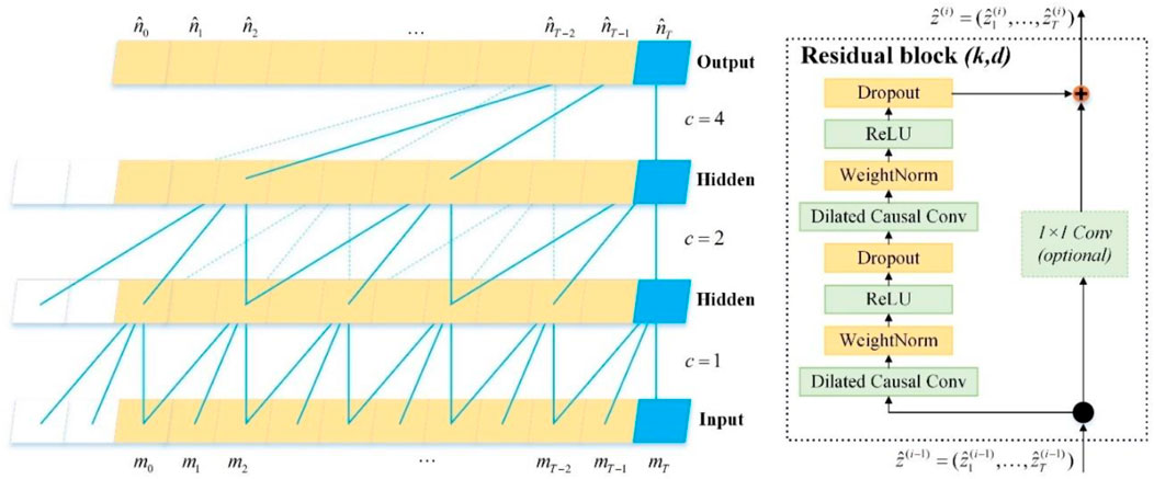
FIGURE 1. The TCN network structure.

NBeats

NBeats was proposed by the Bengio team in 2020. The model does not require complex application background knowledge. And only through simple training, its prediction accuracy can reach up to 3% higher than that of the M4 competition champion (Slawek, 2020). And it also has very good interpretability. The NBeats model structure is shown in Figure 2.

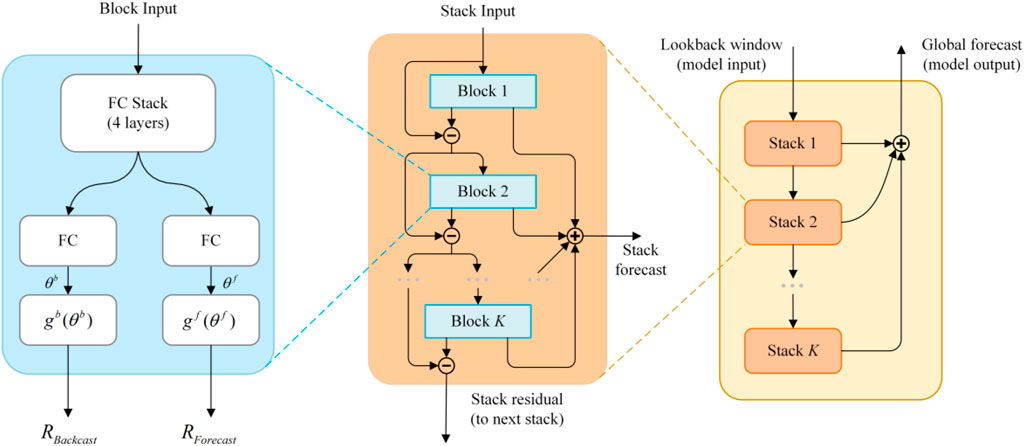
FIGURE 2. The NBeats model structure.

It can be seen from Figure 2 that NBeats has a hierarchical multi-level structure. The basic units in the first layer and the second layer are stacks and blocks, respectively. The sum of multiple stacks constitutes the final output of NBeats. The underlying unit Block is usually composed of a fully connected neural network, namely the FC Stack in Figure 2, activated by 4 layers of ReLU (Guo et al., 2022) and 2 independent network branches. A simple linear layer gives the final model output, which corresponds to the $R_{Forecast}$ arrow in the figure. The other one has the same structure. Its function is to make a difference with the input of the block and use it as the input of the next block, so as to remove the information in the input features that are not highly related to the prediction, which corresponds to the $R_{Backcast}$ arrow in the figure. The specific calculation is as follows:

Where: $p$ is the input vector of Block; $V$ is the intermediate output of $p$ processed by the multi-layer fully connected layer; $W^f$ and $W^b$ are the parameter matrices of fully connected network in order to get the forward prediction coefficient ${\theta }^f$ and backward prediction coefficient ${\theta }^b$; $V_f$ and $V_b$ are the forward and backward basis vectors, respectively, since the parameters ${\theta }^f$ and ${\theta }^b$ have different dimensions; the output $R_{Forecast}$ is the linear transformation of the intermediate variable ${\theta }^f$; $V_f$ is the basic vector representing the output, which can be determined by automatic learning or set as Multi-energy load forecasting based on model fusion.

The basic principles and frameworks of TCN and NBeats are given in the above subsections. For different prediction objects or scenarios, the prediction effects of different base models are different. In order to maximize the comprehensive prediction effect, it is necessary to assign different weights to different sub-learners in different prediction ranges, that is, the comprehensive output is given by:

Where: $S_f$ is the complete set of models used for load forecasting; $s$ is the input feature sequence after UMAP processing; ${\omega }_f$ is the dynamic weight for sub-learner model $f$, and its value can be determined by a fully-trained neural network with softmax as the output unit. Therefore, the multi-energy load forecasting model of the IES can be illustrated as the schematic diagram shown in Figure 3.

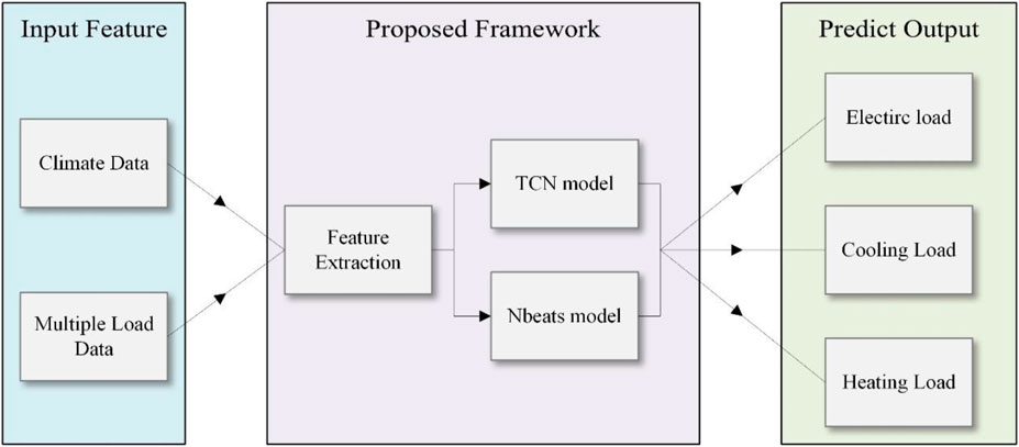
FIGURE 3. Schematic diagram of proposed forecasting model.

The specific training process is described as follows:

Step I. Input the multi-energy load forecasting data samples, and initialize UMAP, TCN, NBeats parameters;

Step II. Perform the dimensionality reduction of the feature data using the UMAP algorithm;

Step III. For episode in max_eps.

a) Given different time window data, train TCN and NBeats sub-models, respectively,

b) Adjust the weights of different forecasting models by gradient descent algorithm according to the prediction results.Step IV. Obtain the final multi-energy load forecasting model and weights for the sub-models by training.

Performance evaluation results of the proposed forecasting model

System description

The test IES studied in this paper is shown in Figure 4, which is extracted from the Engineering Research Center at Tempe campus of Arizona State University and mainly composed of electricity, cooling and heating loads. The 6-years electricity, cooling and heating load data from 2016 to 2021 (http://cm.asu.edu/) are used in this paper, which includes 19-dimensional features such as hourly cooling, heating and electrical load data, the number of rooms, the number of light bulbs, gasoline consumption, and Green House Gas (GHG), etc. The meteorological data of the corresponding area is extracted from the national oceanic and atmospheric administration (NOAA) (https://www.ncei.noaa.gov/), which includes a total of 14 dimensional features, such as hourly altimeter values, dew point temperature, dry bulb temperature, precipitation, pressure change, pressure trend, relative humidity, sea level pressure, surface pressure, visibility, wet bulb temperature, wind direction, gust wind speed, and wind speed. The time interval of the dataset is 1 h, with a total of 52,608 pieces of data, of which the first 75% are used as the training set, and the last 25% are used as the validation set.

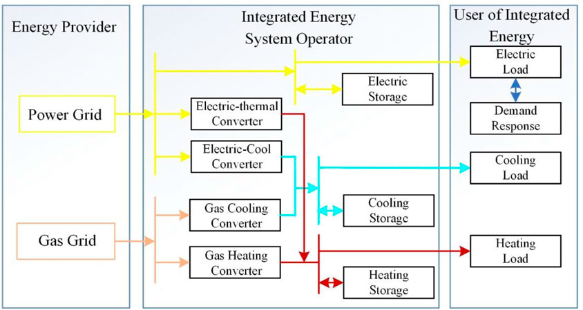
FIGURE 4. Structure of the test integrated energy system.

Data preprocessing

Before load forecasting, the collected data needs to be preprocessed, including the processing of missing data and data normalization. In the process of data collection, data can usually be lost due to communication interferences and other reasons. Here, the missing data is assigned to the observation value of the previous moment.

Different input variables always have different dimensions and value ranges. If the original raw data is directly applied to model training, the forecasting results may be unsatisfactory. Therefore, the data needs to be normalized before model training. The normalization formula is as follows:

Where: $x_i^{\ast }$ and $x_i$ represent the values before and after normalization, respectively; $x_{min}$ and $x_{max}$ represent the minimum and maximum values of the specific variable in the whole sample dataset. The value range of each variable after normalization will be [0,1].

In order to verify the effectiveness of the proposed feature extraction method and the data-driven multi-energy load forecasting model based on TCN-NBeats, the results of different feature processing methods and different forecasting models are then compared in detail.

Comparison between different feature extraction methods

Taking the data of 2016 as an example, Figure 5 shows the correlation coefficient between the cooling, heating and electrical load and meteorological data, Figure 6 shows the correlation coefficient between the cooling, heating and electrical load information. The correlation coefficient between the two variables can be calculated as:

Where: $CR$ represents the correlation coefficient; $Cov$ represents the covariance; D represent the variance; and $E$ represents the mathematical expectation/mean.

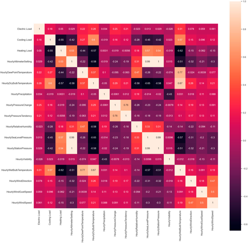
FIGURE 5. Correlation between cooling, heating and electrical load and the meteorological data.

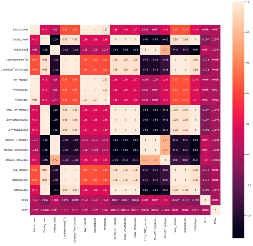
FIGURE 6. Correlation between cooling, heating and the electrical load information.

From the characteristic heat maps of Figure 5 and Figure 6, after calculating the absolute values, the correlation coefficients in the range of 0–0.09 is considered as no correlation, 0.1–0.3 as weak correlation, 0.3–0.5 as medium correlation, and 0.5–1.0 as strong correlation. It can be seen that the multi-energy load prediction (electric, cooling, heating load) are not only related to external features such as meteorological information (for instance, electrical load is moderately correlated with wet bulb temperature (0.31); cooling load is strongly correlated with dry bulb temperature (0.6) and wet bulb temperature (0.57); and heating load is strongly correlated with altimeter setting (0.53) and sea level pressure (0.57)), but also coupled with other load types (for example the electrical load (kW) is moderately correlated with combined mmBTU (0.44) and combined tons carbon (0.44); the cooling load is strongly correlated with the combined mmBTU (0.95) and combined tons carbon (0.95); and the heating load is strongly correlated with cooling load (-0.55)). Therefore, when considering the cooling, heating and power load forecasting problem, the joint prediction of multi-energy loads can better reflect the coupling effect of multiple energy types, and utilize the comprehensive feature information to improve the model accuracy.

Comparisons of single-energy forecasting and multi-energy joint forecasting

In order to verify the effectiveness of the proposed model, this paper compares and analyzes the cooling, heating and electrical load prediction results using different feature extraction methods and forecasting algorithms. The feature extraction methods include PCA, mRMR and proposed UMAP in this paper, and forecasting models include LSTM, NBeats and TCN-NBeats proposed in this paper. The Mean Absolute Percentage Error (MAPE) metric is used as the evaluation index to measure the forecasting effect, which can be computed as follows:

Where: $l_i$ is the actual value of the load consumption; ${\widehat{l}}_i$ is the predicted value of the load consumption; and $n$ is the number of samples.

Figure 7 and Table 1 shows the MAPE distribution and average MAPE of the forecast results of cooling, heating and electrical load for the first week of each month in 2020, using different forecast models. In Figure 7, we compare the scenarios in which different forecasting models are applied to separate forecasting for single-energy load and joint forecasting of cooling, heating and electrical load. In terms of annual average MAPE, the results of multi-energy joint forecasting models are more accurate than the separate forecasting models. According to Table 1, due to the randomness of the test dataset, some MAPE of the multi-energy joint forecasting model may be higher than single-energy forecasting as shown through the highlighted values. However, the annual average MAPE can fully reflect the effectiveness of the joint forecasting. The improvement of the Nbeats is the most significant, which reduces the average annual MAPE from 5.7 to 4.6%, demonstrating that it is suitable for multi-energy load forecasting. The TCN-NBeats ensemble learning model proposed in this paper has a better performance in majority month, and the MAPE of cooling, heating and electrical load prediction is generally around 3.6%, which is superior to the LSTM and NBeats models. Comparing the 12-months cooling, heating and power load prediction results, it can be seen that the TCN-NBeats model has stronger generalization ability against meteorological changes. In summary, joint forecasting considers the correlation between different load types, and thus further improve the model accuracy, and the proposed TCN-NBeats model better assists the forecasting process and shows significant advantages for its generalization ability.

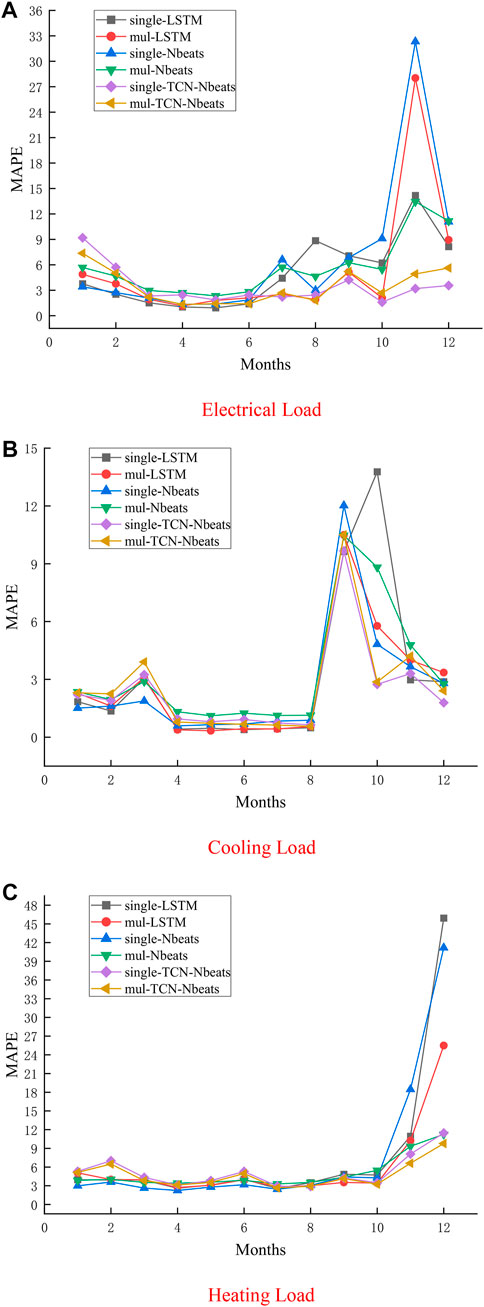
FIGURE 7. MAPE corresponding to each month under different forecasting models.

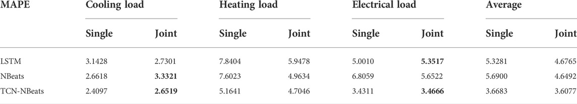
TABLE 1. Comparison of MAPE between single and joint forecasting under different models.

In addition, Table 2 shows the statistical data when different feature extraction methods are combined with the TCN-NBeats multi-energy joint forecasting model, and Figure 8 shows the MAPE distribution of the cooling, heating and electrical load forecasting results for the first week of each month in 2020 under the same condition. It can be seen in Figure 8 that, compared with PCA and mRMR feature extraction methods, UMAP can reduce the feature dimension more while ensuring enough prediction accuracy. In order to further verify the advantages of the UMAP method in terms of dimension reduction, more tests are carried out under different scenarios when the feature dimension is reduced from the original number of 33 to 10, 15, and 20. Table 2 shows that the MAPEs can maintain at about 3.6%, which is very close to the accuracy of the original model without feature reduction. But the feature dimension has been significantly reduced, which will effectively reduce the hyperparameters of the prediction and the training/testing time of the model. To sum up, all of the three feature extraction methods can effectively improve the training speed of the model, but the UMAP method can guarantee its forecasting accuracy while reducing its feature dimension.

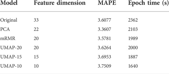
TABLE 2. Different feature extraction and corresponding statistical data under TCN-NBeats model.

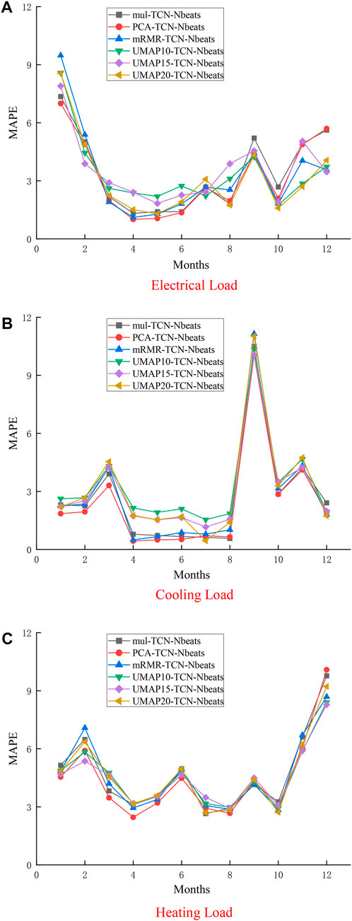
FIGURE 8. Different feature extraction and corresponding monthly MAPE under TCN-NBeats model.

Forecasting results of typical day in different seasons

In different seasons, due to the climatic and meteorological differences, the fluctuation patterns of cooling, heating and electrical loads are quite different. In order to verify the reliability of the multi-energy load forecasting model proposed under different seasons, one typical day is selected for each season for illustration (due to page limit, only summer and winter forecasting results are shown in Figure 9 and Figure 10, respectively). The average MAPE for load forecasting in different seasons under different models are shown in Table 3.

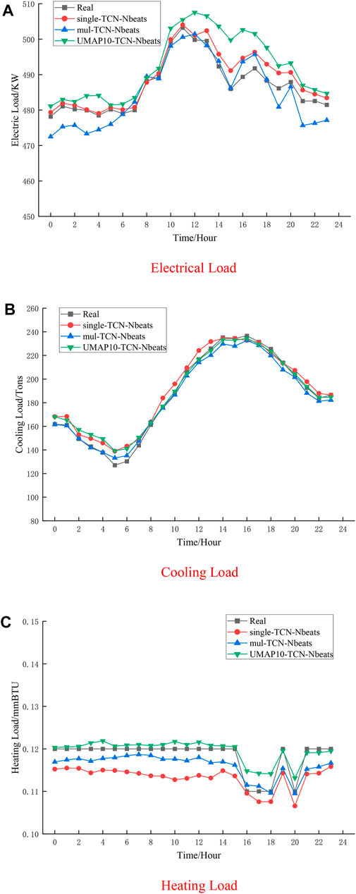
FIGURE 9. Typical daily load forecasting curve (Jun. 1st, 2021).

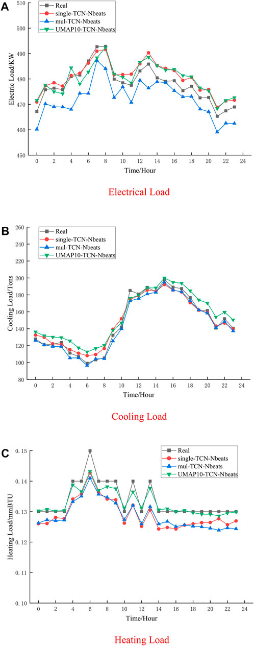
FIGURE 10. Typical daily load forecasting curve (Dec. 1st, 2021).

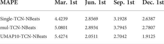
TABLE 3. Average MAPE under different models in different seasons.

Combined the data in both two Figures and the Table, it can be seen that the prediction accuracy is improved under the joint forecasting model of cooling, heating and electricity, and the improvements in summer, autumn and winter are more significant than spring. The TCN-NBeats joint forecasting model with UMAP dimensionality reduction to 10 shows an average MAPE of 5.42% in spring typical day, which is higher than that of both multiple energy TCN-NBeats model and the single-energy forecasting model. The reason is that there are no specific correlations between electrical and cooling loads during spring of the selected dataset, thus, the joint forecasting may interfere the prediction. For winter months, the heating demand is large, most models have lower prediction accuracy. In this case, the TCN-Nbeats multi-energy joint forecasting model using UMAP dimensionality reduction to 10 has an average MAPE of 1.91%, which shows an improvement of 0.72 and 0.87%, compared to the single-energy prediction models and no feature processing, respectively.

Conclusion

This paper focuses on the multi-energy joint forecasting of cooling, heating and electricity loads in IES, and a novel data-driven multi-energy load forecasting model is proposed, which consists of feature dimensionality reduction and ensemble learning-based load prediction. Based on the correlation analysis between the cooling, heating and electrical loads, the UMAP feature extraction method is utilized to reduce the complexity of the model and improve the training and forecasting speed. A TCN-NBeats ensemble learning model is then proposed, which improves the generalization ability of multi-energy load prediction while improving the overall prediction accuracy. The cooling, heating and electrical load forecasting case study shows that the UMAP-based feature extraction method is much superior to PCA, mRMR methods; and the proposed TCN-NBeats multi-energy joint forecasting is more accurate comparing to the traditional single-energy load forecasting methods, also shows great advantages over other machine learning models, such as LSTM, Nbeats, etc.; and the forecasting accuracy will be improved under different seasons using the proposed model.

Data availability statement

The original contributions presented in the study are included in the article/Supplementary Material, further inquiries can be directed to the corresponding author.

Author contributions

Conceptualization, YY, JL, and XL. Methodology, JL and XL. Software, YY. Validation, YY and SL. Formal analysis, ZW. Data curation, CY. Writing—original draft preparation, YY and ZW. Writing—review and editing, KY, ZW, XL, and SL. Supervision, YY and JL. Funding acquisition, XL. All authors have read and agreed to the published version of the manuscript.

Funding

This work was supported in part by the National Key Research and Development Program of China under Grant 2018YFB0905000, and the Guangdong Energy Group Science and Techology Research Institute Co., Ltd.’s Project “Research on high-efficiency intelligent multi-supply technology for integrated electric heating cold and water”.

The funder had the following involvement in the study: Conceptualization, YY; software, YY; validation, YY and SL; formal analysis, ZW; data curation, CY.; writing—original draft preparation, YY.; writing—review and editing, SL; supervision, YY.

Conflict of interest

Authors YY, SL, ZW, and CY were employed by Guangdong Energy Group Science and Technology Research Institute Co, Ltd.

The remaining authors declare that the research was conducted in the absence of any commercial or financial relationships that could be construed as a potential conflict of interest.

Publisher’s note

All claims expressed in this article are solely those of the authors and do not necessarily represent those of their affiliated organizations, or those of the publisher, the editors and the reviewers. Any product that may be evaluated in this article, or claim that may be made by its manufacturer, is not guaranteed or endorsed by the publisher.

References

Chen, Z., Liu, J., and Liu, X. (2021). GPU accelerated power flow calculation of integrated electricity and heat system with component-oriented modeling of district heating network. Appl. Energy 305, 117832. doi:10.1016/j.apenergy.2021.117832
Cho, K., Merrienboer, B., Bahdanau, D., et al. (2014). On the properties of neural machine translation: Encoder-decoder approaches. Proceed. SSST-8, 103–111. doi:10.3115/v1/W14-4012
Guo, J., Zhang, P., Wu, D., Liu, Z., Liu, X., Zhang, S., et al. (2022). Multi-objective optimization design and multi-attribute decision-making method of a distributed energy system based on nearly zero-energy community load forecasting. Energy 239 (C), 122124. doi:10.1016/j.energy.2021.122124
He, K., Zhang, X., Ren, S., et al. (2016). ResNet-Deep residual learning for image recognition. Seattle: CVPR.
Hochreiter, S., Schmidhuber, J., et al. (1997). Long short-term memory. Neural Comput. 9, 1735–1780. doi:10.1162/neco.1997.9.8.1735
LeCun, Y., Boser, B., Denker, J. S., et al. (1989). Backpropagation applied to handwritten zip code recognition. Neural Comput. 1 (4), 1989. doi:10.1162/neco.1989.1.4.541
Liao, Z., Huang, J., Cheng, Y., Li, C., and Liu, P. X. (2022). A novel decomposition-based ensemble model for short-term load forecasting using hybrid artificial neural networks. Appl. Intell. (Dordr). 2022, 11043–11057. doi:10.1007/s10489-021-02864-8
Liu, J., Chen, J., Wang, C., Chen, Z., and Liu, X. (2020). Market trading model of urban energy internet based on tripartite game theory. Energies 13 (7), 1834. doi:10.3390/en13071834
Liu, J., Fang, W., Zhang, X., and Yang, C. (2015). An improved photovoltaic power forecasting model with the assistance of aerosol index data. IEEE Trans. Sustain. Energy 6 (2), 434–442. doi:10.1109/tste.2014.2381224
Liu, J., Zhao, H., and Liu, J. (2019). Medium term load forecasting based on cointegration-granger causality test and seasonal decomposition. Automation Electr. Power Syst. 43 (1), 73–80. doi:10.7500/AEPS20180629013
Liu, X., Liu, J., and Chen, J. (2021). Expansion planning of community-scale regional integrated energy system considering grid-source coordination: A cooperative game approach. Ener. Proceed. 18, 2021. doi:10.46855/energy-proceedings-9215
Mikolov, T., Sutskever, I., Chen, K., et al. (2013). Distributed representations of words and phrases and their compositionality. Adv. Neural Inf. Process. Syst. 26, 3111. doi:10.48550/arXiv.1310.4546
Nair, V., and Hinton, G. E. (2010). Rectified linear units improve restricted Boltzmann machines. Maryland.ICML
Rochareis, A. J., and Alvesdasilva, A. P. (2005). Feature extraction via multiresolution analysis for short-term load forecasting. IEEE Trans. Power Syst. 20 (1), 189–198. doi:10.1109/tpwrs.2004.840380
Slawek, S. (2020). A hybrid method of exponential smoothing and recurrent neural networks for time series forecasting. Int. J. Forecast. 36 (1), 75–85. doi:10.1016/j.ijforecast.2019.03.017
Song, Y., Yang, Y., He, Z., Li, C., and Li, L. (2019). A hybrid forecasting system based on multi-objective optimization for predicting short-term electricity load. J. Renew. Sustain. Energy 11 (6), 066101. doi:10.1063/1.5109213
Sun, X., Ouyang, Z., and Dong, Y. (2017) Short-term load forecasting model based on multi-label and BPNN,” in Int. Conf. Life Syst. Model. Simul. Int. Conf. Intelligent Comput. Sustain. Energy & Environ., 25. Singapore, 263. doi:10.1007/978-981-10-6370-1_26
Tang, J., Liu, J., Zhang, M., et al. (2016). “Visualizing large-scale and high-dimensional data,” in Proceedings of the 25th international conference on world wide web, 287.
Teng, Q., and Li, Y. (2015). Nonparametric nearest neighbor descent clustering based on delaunay triangulation. Comput. Sci., 04837. arXiv:1502.04837. doi:10.48550/arXiv.1502.04837
Vanting, N. B., Ma, Z., and Jrgensen, B. N. (2021). A scoping review of deep neural networks for electric load forecasting. Energy Inf. 4 (2), 49. doi:10.1186/s42162-021-00148-6
Wang, S., Wang, S., Chen, H., and Gu, Q. (2020). Multi-energy load forecasting for regional integrated energy systems considering temporal dynamic and coupling characteristics. Energy 195, 116964. doi:10.1016/j.energy.2020.116964
Wang, S., Wu, K., Zhao, Q., Feng, L., Zheng, Z., et al. (2021). Multi-energy load forecasting for regional integrated energy systems considering multi-energy coupling of variation characteristic curves. Front. Energy Res. 9, 635234. doi:10.3389/fenrg.2021.635234
Yang, D., and Wang, M. (2021). Optimal operation of an integrated energy system by considering the multi energy coupling, AC-DC topology and demand responses. Int. J. Electr. Power & Energy Syst. 129 (2), 106826. doi:10.1016/j.ijepes.2021.106826
Zhang, G., Bai, X., and Wang, Y. (2021). Short-time multi-energy load forecasting method based on CNN-seq2seq model with attention mechanism. Mach. Learn. Appl. 5, 100064. doi:10.1016/j.mlwa.2021.100064
Zhang, T., Li, H., and Hui, Q. (2019). Integrated load forecasting model of multi-energy system based on Markov chain improved neural network. 2019 11th International Conference on Measuring Technology and Mechatronics Automation (ICMTMA). IEEE, Qiqihar, China, Apr 28-29, 1–6. doi:10.1109/ICMTMA.2019.00106
Keywords: integrated energy system (IES), data-driven, multi-energy load forecasting, feature dimensionality reduction, ensemble learning, UMAP (uniform manifold approximation projection), TCN, NBeats
Citation: Yao Y, Li S, Wu Z, Yu C, Liu X, Yuan K, Liu J, Wu Z and Liu J (2022) A novel data-driven multi-energy load forecasting model. Front. Energy Res. 10:955851. doi: 10.3389/fenrg.2022.955851
Received: 29 May 2022; Accepted: 28 June 2022;
Published: 22 July 2022.
Edited by:
Ningyi Dai, University of Macau, ChinaReviewed by:
Zitian Qiu, University of Liverpool, United KingdomZiyu Fan, University of Liverpool, United Kingdom
Copyright © 2022 Yao, Li, Wu, Yu, Liu, Yuan, Liu, Wu and Liu. This is an open-access article distributed under the terms of the Creative Commons Attribution License (CC BY). The use, distribution or reproduction in other forums is permitted, provided the original author(s) and the copyright owner(s) are credited and that the original publication in this journal is cited, in accordance with accepted academic practice. No use, distribution or reproduction is permitted which does not comply with these terms.
*Correspondence: Jun Liu, eeliujun@mail.xjtu.edu.cn