The impact of rooftop solar on wholesale electricity demand in the Australian National Electricity Market

1 Introduction

Increasing concerns about carbon emissions and climate change have motivated energy transition and the continuing adoption of renewable energy over the last few decades (Australian Energy Market Operator, 2022). Consumers have also started managing their own energy by investing in distributed energy resources (DERs) (O’Shaughnessy et al., 2021). These circumstances have led to ongoing installations of rooftop solar photovoltaics (PVs). Specifically, rooftop PV installations participating in Australia’s National Electricity Market (NEM) have been increasing during the last decade, as shown in Figure 1below. Consequently, Australia has the most rooftop PVs installed per capita of any country in the world (Australian Energy Market Operator and Energy Networks Australia, 2019; Shaw-Williams et al., 2019; Zander et al., 2019; Wilkinson et al., 2021).

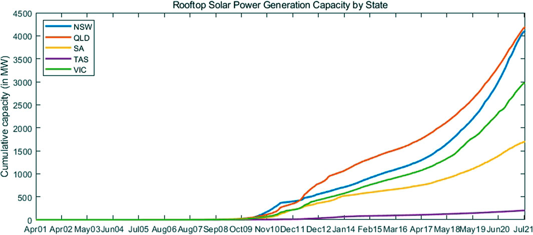
FIGURE 1. Cumulative small-scale solar generation capacity from April 2001 to August 2021. Source: Clean Energy Regulator and the authors’ calculation.

This phenomenon is very likely to contribute to negative daytime electricity prices. For example, South Australia (SA) witnessed a record number of negative prices in December 2020 due to mild weather, record power generation from rooftop solar, and a high level of output from large-scale renewable generation (Australian Energy Market Operator, 2021), with the price even reaching A$–679.30 at 1:30p.m. on 18 December 2021.

Examining whether and how rooftop solar affects intra-day and inter-day patterns of power demand and, more generally, the wholesale electricity market, is of great significance for regulators and investors in utilities.

Much literature addresses how rooftop solar adoption is determined rather than the impact of increasing rooftop solar PV installations. Collier et al. (2023) identify population traits, residential density, size, type and tenure, and power consumption patterns as significant factors influencing solar PV uptake. Zhang et al. (2023) find evidence of neighbourhood-level spatial interaction effects in the determination of residential solar PV adoption. Ros and Sai (2023) establish regression models for household solar PV demand. O’Shaughnessy et al. (2021) investigate the state policy interventions and business models accelerating the rooftop solar adoption in the low-income households. Alrawi et al. (2022) survey the public perception towards rooftop solar PV installations in Qatar, while Zander et al. (2019) examine the impact of financial incentives on residential rooftop solar PV adoption in Australia.

Current literature rarely focuses solely on rooftop solar energy. Most studies examine the impact of renewable energy or distributed energy resources. Shen et al. (2023) analyze the impact of co-adopting EV, rooftop solar PV, and home battery storage. Earle et al. (2023) propose a promising strategy of combining traditional energy-efficiency upgrades and behind-the-meter DERs to achieve residential electrification. López Prol et al. (2020), Sensfuß et al. (2008), Cardenas et al. (2017), and Csereklyei et al. (2019) document that increased adoption of intermittent renewable energy, including rooftop solar, is very likely to reduce wholesale electricity prices.¹ There are also related studies in the Australian context (Blakers et al., 2021; Gonçalves and Menezes, 2022; Srianandarajah et al., 2022). El-Adaway et al. (2020) and Perez-Arriaga (2016) focus on the effect of energy transition and distributed energy resource penetration, while Quint et al. (2019) review various challenges resulting from distributed energy resources.

In the Australian context, the impact of small-scale power generation from renewable energy across the whole national market is under-explored. Higgs et al. (2015), Rai and Nunn (2020), and Alsaedi et al. (2020) investigate the effect of utility-scale VRE generation.² Besides, the literature focusing on regional markets in the NEM is abundant. Wu et al. (2023) try to identify predictors of electricity demand with consideration of COVID-19 lockdowns in Victoria. Wilkinson et al. (2021) demonstrate empirically the impact of rooftop solar on intra-day wholesale electricity prices of Western Australia. Simshauser (2022) discusses the peak load problem associated with high penetration of rooftop solar PVs in the NEM’s Queensland region. Al Khafaf et al. (2022) analyze the impact of smart meters on household energy consumption in Victoria. The exception we are aware of is Mwampashi et al. (2022) who focus on the impact of solar generation, both large-scale and small-scale, on electricity spot prices and the corresponding volatility in the NEM.

Thus, there have been few comprehensive analysis on the impact of rooftop solar generation in the Australian National Electricity Market. We investigate whether and how rooftop solar installations affect wholesale power demand which is the intermediary channel in the relationship between power generation from renewable energy and electricity pricing, complementing the research in this area.

Additionally, most literature in this area has focused on short-term electricity demand projection Hsiao (2014), Aneiros et al. (2016), Lindberg et al. (2019) suggest the feature of more renewable energy sources should be considered in long-term power load forecasting. Nti et al. (2020) point out that most electricity forecasting models with best performances apply artificial intelligence. Al Mamun et al. (2020) review different electric load prediction techniques based on machine learning, while Vanting et al. (2021) evaluate different projection methodologies using deep neural networks. Franco and Sanstad (2008) and McFarland et al. (2015) model and predict electricity consumption in the context of the United States, giving consideration to climate change and consequent temperature increases. Morcillo et al. (2022) estimate nearly 20% saving in future energy bills with the adoption of solar PVs based on a system dynamics model.

However, there are a limited number of studies forecasting the intra-day patterns of electricity spot demand in the long term. We have provided electricity spot demand projection in the post-pandemic era on a half-hourly basis, emphasizing the impact of rooftop solar PV adoption.

To the best of our knowledge, ours is one of the first studies in the context of the NEM that focuses on rooftop solar PV systems as a typical example of small-scale renewable energy generation. We find that a 1 MW increase in rooftop solar generation corresponds with 0.5–0.6 MW decrease of spot-demand deviation from its seasonal patterns on a half-hourly basis in individual state markets of the NEM. Moreover, our study also contributes to predicting intra-day electricity demand patterns in the long term given the impact of increasing solar rooftop uptakes. We conclude that the peak of intra-day electricity consumption will gradually move to form around dusk due to the growth of solar generation from rooftop PVs.

In Section 2 of this paper, we introduce the various methods applied through the analysis, before describing our data in Section 3. Section 4 shows the main results of the study, preceding the conclusion in Section 5.

2 Methodology

Figure 2 demonstrates the procedure of this empirical study. The goal of this study is to visualize (Box 1) and to quantify (Box 4) the impact of rooftop solar installations on the spot demand of individual states in the Australian National Electricity Market. Based on the models with consideration of solar rooftop, we also aim to forecast spot electricity demand during 2019–2034 (Box 7).

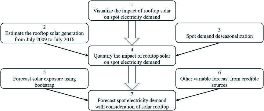
FIGURE 2. Flow chart of the whole analysis.

To achieve the goal of Box 4, we develop a novel approach in Section 2.1 to estimate rooftop solar generation based on total daily global solar exposure and half-hourly effective working hours of rooftop solar PV panels (Box 2). Because the data on rooftop solar generation from July 2009 to July 2016 is missing. Specifically, total daily global solar exposure is referred to as the total amount of solar energy falling on a horizontal surface of unit area for a day. Effective working hours of rooftop solar PV panels are calculated as the ratio of rooftop solar generation over the solar power generation capacity of small-scale PV systems.

Given that seasonal factors may affect the results, half-hourly electricity demand as the dependent variable should be deseasonalized (Box 3) before quantifying the effect of rooftop solar on wholesale electricity demand in the NEM through regression models (Box 4). Section 2.2 details the procedure for deseasonalizing spot-demand data.

The method in Section 2.3 is adopted to speculate on the possible values of daily solar exposure in the future (Box 5). The forecast of other variables is from credible sources (Box 6), such as state governments’ official websites. Section 2.4 presents the models built for capturing the effect of distributed solar power generation facilities on deseasonalized spot demand in each Australian state (Box 4) and also for forecasting spot demand in the next 15 years (Box 7).

2.1 Estimating rooftop solar generation

This section corresponds with Box 2 in the flow chart of Figure 2. We aim to estimate the generation from rooftop PVs for each market, taking into account the generation during the daytime (i.e., half-hourly generation) and information on the small-scale (systems up to 100 kW) solar power generation capacity for each market (available on a monthly basis). Unfortunately, the Australian Energy Market Operator (AEMO) only provides estimates³ on half-hourly rooftop solar generation starting from August 2016. We therefore decided to estimate the half-hourly solar power generation for the remaining sample period, from July 2009 to July 2016.

If power generation from rooftop PVs is not available for a certain 30-min time interval (t, d, y), our estimates are based on total daily global solar exposure and effective working hours of PV panels during a specific 30-min interval (t) on the corresponding date (d) in different benchmark periods (y + n) for each state (i). Benchmark periods are those years where data on rooftop solar PV generation is available from the AEMO.

First, effective working hours of PV panels in benchmark years (h_i,t,d,y+n) can be approximated by using the ratio of rooftop solar power generation (RftPVGen_i,t,d,y+n) to the generation capacity of rooftop PV panels (GenCp_i,m,y+n) in the corresponding month.

RftPVGen_i,t,d,m,y+n is officially estimated by the AEMO, while GenCp_i,m,y+n is collected by the Clean Energy Regulator. Due to it taking 12 months for individuals to register for small-scale technology certificates, at which point their generation capacity appears in the data⁴, rooftop PV panel generation capacity for the most recent year may be underestimated. Therefore, the benchmark period applied here ends in July 2020 to avoid overestimating the effective working time of rooftop PV panels.

Second, by summing the effective working hours for each 30-min interval, we obtain the effective working time for a certain date (d). A constant is inferred from the average ratio of daily effective working time over the corresponding total daily global solar exposure (SolarExpo) from August 2016 to July 2020 when both data are available.

The half-hourly distribution of the effective working time of PV panels during a day is calculated as the proportion of half-hourly working time over total daily working time. To minimize the effect of unusual observations, we first average the effective working duration inferred from the same 30-min intervals in a 31-day window that moves in 1-day steps. Then we take the mean value of the smoothed ratios on the same dates from different benchmark years, i.e., August 2016–July 2017, August 2017–July 2018, August 2018–July 2019, and August 2019–July 2020.

Last, the estimated power generation of rooftop solar PVs is the product of rooftop solar generation capacity for the corresponding month (GenCp_i,m,y), the corresponding total daily global solar exposure (SolarExpo_i,d,y), the constant inferred from historical data, and intra-day patterns of the effective working time of rooftop PV panels (Dist_i,t,d).

2.2 Demand deseasonalization

This section details Box 3 in the flow chart of Figure 2. In estimating the seasonal pattern of power demand, half-hourly demand observations are classified by the days of the week as well as the corresponding month, for example, Mondays in January, Tuesdays in January, …, Wednesdays in February, …, Sundays in December. Public holidays are treated as Sundays. This classification considers weekly as well as yearly patterns. Initially, 84 (7 × 12) groups are classified.

Given that this study deals with half-hourly spot-demand data, we also need to model the intra-day periodicity. In 1 day, there are 48 half-hourly data points, which are again classified by days of the week and months of the year (e.g., 11a.m. on Mondays in January). Thus, the final number of groups is 4,032 (84 × 48). We decided to choose a non-parametric approach, where the seasonal pattern for each group is calculated as the mean value in the group. For example, the average demand during 12–12:30p.m. on Mondays in January is regarded as the typical demand for this specific trading interval. Estimated seasonal components suggest that for each market, spot electricity demand exhibits very different intra-day patterns depending on the season and time of the year.⁵ Demand exhibits more peaks in summer due to periods of extreme temperature, and also the wide use of air conditioners. This is why it seems more appropriate to estimate separate weekly short-term seasonal components (STSCs) for different months of the year instead of just a single weekly intra-day pattern. Note, however, that this estimation method is typically the case for spot electricity markets (see, for example, Pilipovic, 1997; Geman and Roncoroni, 2006; Weron, 2006; Bierbrauer et al., 2007; Janczura et al., 2013; Yan and Trück, 2020).

As we also try to forecast spot demand in the following years, the impact of the COVID-19 pandemic should be taken into consideration. Most countries implemented lockdowns to reduce transmission of the virus at the beginning of the pandemic, including Australia, which announced a “national lockdown” on 23 March 2020. Restrictions commonly seen in lockdowns included “stay at home” orders and work-from-home arrangements. This can be expected to change various aspects of daily routines including electricity usage. Thus, different STSCs are estimated before and after the lockdown date of 23 March 2020.

2.3 Bootstrap forecast

This section describes the steps of Box 5 in the flow chart of Figure 2. The reason why the forecast of future solar exposure is based on a non-parametric approach is that solar exposure has not been the focus of any institution tracking energy prices or consumption to our knowledge. In contrast, forecasted values of most other variables can be found from credible public sources.

Our solar exposure forecast contains two components: one seasonal and the other stochastic. The seasonal component is estimated as the mean monthly pattern. The stochastic component is simulated using the stationary bootstrapping method of Politis and Romano (1994). As pointed out by Laker et al. (2017), stationary bootstrapping has the advantage over traditional block bootstrapping that it retains the stationarity of the original dataset and accounts for potential serial dependence and seasonality.

The bootstrapping procedure contains the following steps. For each forecast day, we locate the same days in historical years in our dataset and apply a ± 45 days window (i.e., 90 days in total) to determine the sample set to bootstrap from.⁶ After that, a random block length is determined from a geometric distribution (G(p)) where the mean block length is $\frac{1}{p}$. We apply the method proposed by Politis and White (2004) and Patton et al. (2009) to choose the mean block length with an automatic procedure by examining the serial dependence in the original time series. This step is repeated until the length of the future period we are interested in is reached. Compared to the standard stationary bootstrapping method, which conducts resampling using the full historical data, the dynamic sampling window provides better information relevance and accounts for potential remaining seasonality. Finally, the estimated seasonal component and the bootstrapping results are combined to construct a forecast of future solar exposure.

2.4 Modelling equations

This section provides the details of Box 4 and Box 7 in the flow chart of Figure 2. To realize the goal in Box 4, we build the following model.

where DesDemand measures the difference between actual half-hourly demand and its seasonal pattern,⁷RooftopSolarGen denotes the estimated half-hourly rooftop solar generation, ⁸ and CtrlVar are control variables.

To quantify the effect of the national lockdown due to COVID-19 on the relationship between deseasonalized spot demand and rooftop solar, we estimate the following model based on the sample data from 1 January 2018 to 30 June 2022 so that the number of dates before and after the national lockdown is similar.

DesDemand measures the difference between actual half-hourly demand and its seasonal pattern.⁹ Different short term seasonal components are estimated before and after the national lockdown due to changes to people’s daily lives. I_covid equals 1 (0) if t is after (before) 23 March 2020. RooftopSolarGen denotes the half-hourly rooftop solar generation, and CtrlVar are control variables.

Concerning the goal in Box 7, we forecast spot demand in the next 15 years following Equation 7, after regressing deseasonalized spot demand on considered independent variables and estimating the coefficients in Equation 5.

where STSC represents short-term seasonal components calculated with the method described in Section 2.2; and $\tilde{\alpha }$, $\tilde{\beta }$, and $\widetilde{{\mathit{\gamma }}^{\prime }}$ are the coefficients estimated through regressions.

3 Data

Data of half-hourly spot demand and estimated solar power generation from rooftop PVs is publicly available from the AEMO. Data of total daily global solar exposure and half-hourly dry-bulb temperature comes from the Bureau of Meteorology, an agency of the Australian federal government. The capacity data for small-scale installations is from the Clean Energy Regulator, an Australian statutory authority. Data on gross state product (GSP), population, the consumer price index (CPI) on electricity, and the number of households for individual state markets is from the Australian Bureau of Statistics. Descriptive statistics of key variables are displayed in Supplementary Tables A2, A3.

Our forecast of rooftop solar generation is based on Equation 4, while we estimate future solar exposure employing the bootstrap method introduced in Section 2.3. The predicted capacity of rooftop PVs is from the Australian Energy Market Operator (2022), and we have averaged the values under four scenarios:¹⁰ “slow change”, “progressive change”, “step change”, and “hydrogen superpower”. The projection of daily temperature for the next 15 years is from the Climate Change in Australia website (http://www.climatechangeinaustralia.gov.au/) which is the joint work of the Commonwealth Scientific and Industrial Research Organisation (CSIRO) and Bureau of Meteorology. The forecast of GSP and CPI is from the treasury of each state. The projection of NSW population is from the NSW Department of Planning and Environment. The forecast of population and GSP for the Australian Capital Territory is from the ACT 2022–2023 Budget Outlook. The population projections for Queensland and Tasmania are from the respective state treasuries, while the projection for SA is from the state’s online planning and development system. The estimated growth rate of the population for Victoria is from the Victorian Department of Environment, Land, Water and Planning. The estimated number of households in the next 15 years are from the Australian Bureau of Statistics.

Given that data on solar power generation from rooftop PVs is not available from July 2009 to July 2016, it is necessary to ensure the estimated solar generation does not deviate too far from actual values before quantifying its impact. Figure 3 shows the comparison between actual and estimated monthly rooftop solar power generation from August 2016 to July 2020, suggesting our method is roughly accurate in estimating aggregate rooftop solar power generation on a monthly basis.

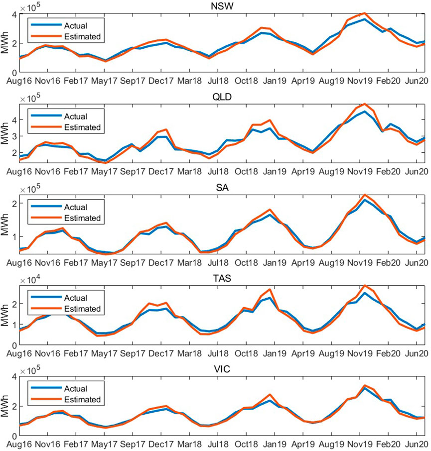
FIGURE 3. Actual and estimated monthly rooftop solar power generation (in MWh). Effective working hours of PV panels are estimated as the average value across the periods from August 2016 to July 2017, August 2017 to July 2018, August 2018 to July 2019, and August 2019 to July 2020.

At the same time, the methodology described in Section 2.1 should not bring systematic errors to the estimation of intra-day solar generation. We have shown the comparison between actual and estimated half-hourly solar generation for each month in Supplementary Figure A1. The actual half-hourly solar generation for each month is the average half-hourly solar generation for the same 30-min intervals, i.e., 12–12:30a.m., 12:30–1a.m., etc., on different days in the same month. The estimated half-hourly solar generation for each month is the product of corresponding rooftop solar generation capacity and the typical working duration calculated as the average working time for the same 30-min intervals, i.e., 12–12:30a.m., 12:30–1a.m., etc., on different days in the same months of four benchmark periods. The comparison suggests that our methodology does not bring substantial biases to the estimation of intra-day patterns for solar generation.

On a half-hourly basis, descriptive statistics of the differences between the rooftop solar power generation estimates inferred from the methodology in Section 2.1 and the corresponding data from the AEMO are displayed in Table 1. Given the scales of actual half-hourly generation from rooftop solar in the third section of Table 1, mean and median values of the (absolute) deviation indicate that our estimates are reasonably good. Among the five states in the NEM, it is most difficult to accurately estimate solar generation in NSW and Queensland, while the inter- and intra-day patterns of solar generation in Tasmania are relatively stable, so that our methodology is better at estimating small-scale solar generation there. More specifically, the average deviation of estimated half-hourly solar generation from its actual values for different 30-min intervals is shown in Supplementary Table A4. Compared to the scale of actual generation, our method does not bring significant biases to the estimation of half-hourly solar generation.

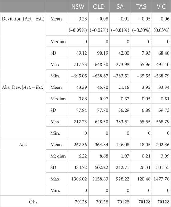
TABLE 1. Descriptive statistics of the differences between the half-hourly rooftop solar generation inferred from effective working hours during benchmark periods and the AEMO generation data. Deviation and absolute deviation are measured in MW.

Therefore, the effective working hours inferred from the method in Section 2.1 can be used to derive estimates for rooftop solar generation on a half-hourly basis for the remaining sample period, i.e., from July 2009 to July 2016, as the comparison from different perspectives does not indicate significant deviation of estimated small-scale solar generation from the actual values. The estimates here are reasonably good.

4 Empirical results

4.1 The effect of rooftop solar generation on demand

As electricity generation from rooftop solar only makes up a small share of total electricity demand in each market, which we will illustrate in the following analysis, to quantify the effect of rooftop solar, first we must confirm whether there is detectable variation in the patterns of power demand due to rooftop solar. This section corresponds with Box 1 in the flow chart of Figure 2.

It is important to acknowledge that despite the significant increase in household installations of solar panels, the energy generated from rooftop solar only accounts for a limited fraction of total demand in most markets between 2009 and 2019. Supplementary Figure A2 shows the percentage of total demand that is generated from solar panels for the markets in NSW, Queensland, SA, Tasmania, and Victoria. These numbers range from less than 3% for Tasmania and a maximum of approximately 6% in NSW and Victoria to a maximum of almost 18% in SA. However, given that the share of actual generation is typically much lower than these maximum values for most of the markets, generation from rooftop solar panels can only be expected to have a limited effect on power demand.

The substantial increase in rooftop solar installations might have played a role in the overall trend of decreasing demand for electricity that is traded through the NEM. Supplementary Figure A3 shows how during our sample period for three major markets—NSW, SA, and Victoria—there has been a declining trend in the market load, i.e., electricity that is traded in the NEM. Interestingly, for Queensland there was an increase in demand throughout 2009–2019.

Given these observations, we would like to have a closer look at the influence of rooftop solar generation on intra-day demand at different times. To do this, we consider two different trading intervals: 1–1:30p.m., when markets are likely to have a maximum share of solar electricity generation, and 8–8:30p.m., when it is very likely that there is no generation from rooftop solar installations.

Figure 4 shows that throughout the sample period the total demand for the 1–1:30p.m. trading interval has decreased more substantially in comparison to the 8–8:30p.m. interval for the markets in NSW, SA, Tasmania, and Victoria. This observation is also proved by the p-values of testing whether the slopes of two trend lines are significantly different. Furthermore, the decrease in demand for the 1–1:30p.m. period is more striking for the markets in SA, Queensland, and Victoria, where a significantly higher share of electricity comes from rooftop solar installations. We also find that demand levels have slightly decreased for the 1–1:30p.m. trading period in Queensland, while demand has increased quite substantially for the 8–8:30p.m. period. Overall, these findings may suggest that the increase in generation from rooftop solar can indeed affect demand patterns.

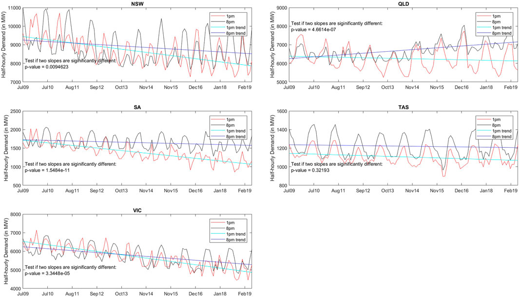
FIGURE 4. Monthly average half-hourly power demand for the 1–1:30p.m. and 8–8:30p.m. trading intervals for NSW, Queensland, SA, Tasmania, and Victoria. The figures also show the corresponding trend line for each trading interval and the considered sample period from 2009 to 2019. Source: AEMO and the authors’ calculations.

The left panels of Figures 5–9 also show the impact of rooftop solar on typical intra-day patterns of electricity demand. We choose two different months: August, a period in winter when electricity is needed for heating, and January, a period in summer when people need electricity for cooling and there is more likely to be sufficient sunshine, longer daytime, and more generation from rooftop solar installations. Both curves display similar patterns, referred to as the duck curve (Simshauser and Akimov, 2019; Wilkinson et al., 2021). Comparing the first (2009–2010), fourth (2012–2013), seventh (2015–2016), and last financial year (2018–2019) of our sample period, we can see deepening troughs in power demand during the daytime in August for NSW, Queensland, SA, and Victoria. Increasing adoption of rooftop solar PV systems and other facilities leads to decreased grid load. Especially for Queensland and SA, which had substantially higher rooftop solar penetration in 2018, the demand trough in the August daytime is almost the same as the daily demand trough around 4a.m. Additionally, the daily demand peak was gradually formed around or even after 4p.m. in January for these states, especially in Queensland and SA, where the demand curve between 8a.m. and 6p.m. changes from convex to concave.

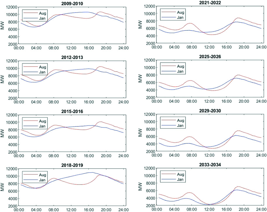
FIGURE 5. The left panel shows intra-day demand patterns in August and January of the first, fourth, seventh, and last financial year of the sample period, i.e., August 2009 and January 2010, August 2012 and January 2013, August 2015 and January 2016, and August 2018 and January 2019. The right panel displays intra-day demand patterns in August and January of the third, seventh, 11th, and last financial year of the forward-looking period, i.e., August 2021 and January 2022, August 2025 and January 2026, August 2029 and January 2030, and August 2033 and January 2034. The half-hourly demand (in MW) is calculated as the average power demand for the same 30-min trading intervals of different days in the corresponding month. The change through time is shown for NSW.

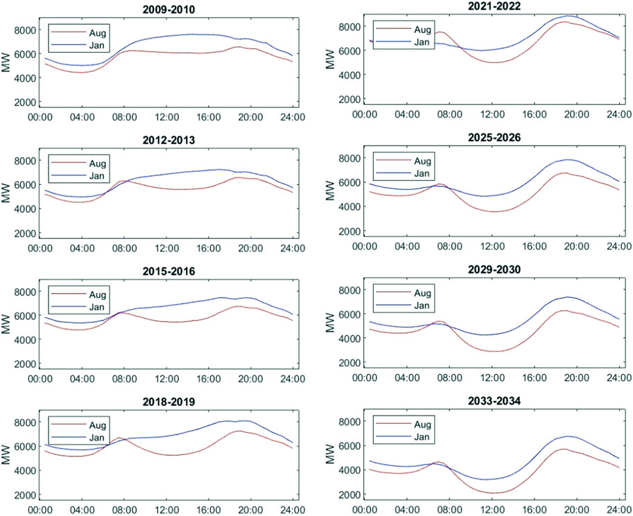
FIGURE 6. The left panel shows intra-day demand patterns in August and January of the first, fourth, seventh, and last financial year of the sample period, i.e., August 2009 and January 2010, August 2012 and January 2013, August 2015 and January 2016, and August 2018 and January 2019. The right panel displays intra-day demand patterns in August and January of the third, seventh, 11th, and last financial year of the forward-looking period, i.e., August 2021 and January 2022, August 2025 and January 2026, August 2029 and January 2030, and August 2033 and January 2034. The half-hourly demand (in MW) is calculated as the average power demand for the same 30-min trading intervals of different days in the corresponding month. The change through time is shown for Queensland.

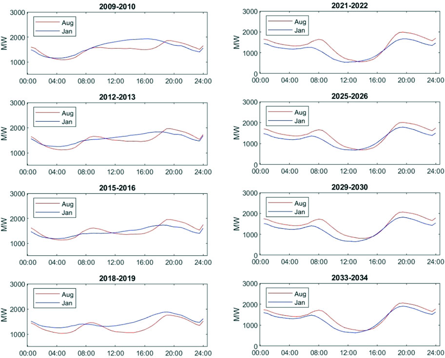
FIGURE 7. The left panel shows intra-day demand patterns in August and January of the first, fourth, seventh, and last financial year of the sample period, i.e., August 2009 and January 2010, August 2012 and January 2013, August 2015 and January 2016, and August 2018 and January 2019. The right panel displays intra-day demand patterns in August and January of the third, seventh, 11th, and last financial year of the forward-looking period, i.e., August 2021 and January 2022, August 2025 and January 2026, August 2029 and January 2030, and August 2033 and January 2034. The half-hourly demand (in MW) is calculated as the average power demand for the same 30-min trading intervals of different days in the corresponding month. The change through time is shown for SA.

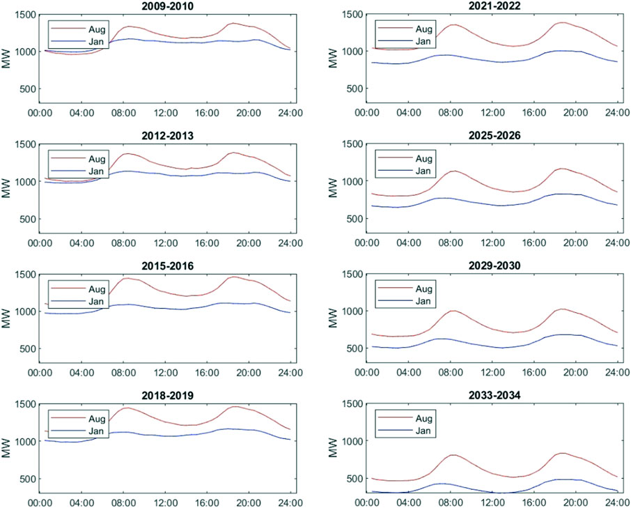
FIGURE 8. The left panel shows intra-day demand patterns in August and January of the first, fourth, seventh, and last financial year of the sample period, i.e., August 2009 and January 2010, August 2012 and January 2013, August 2015 and January 2016, and August 2018 and January 2019. The right panel displays intra-day demand patterns in August and January of the third, seventh, 11th, and last financial year of the forward-looking period, i.e., August 2021 and January 2022, August 2025 and January 2026, August 2029 and January 2030, and August 2033 and January 2034. The half-hourly demand (in MW) is calculated as the average power demand for the same 30-min trading intervals of different days in the corresponding month. The change through time is shown for Tasmania.

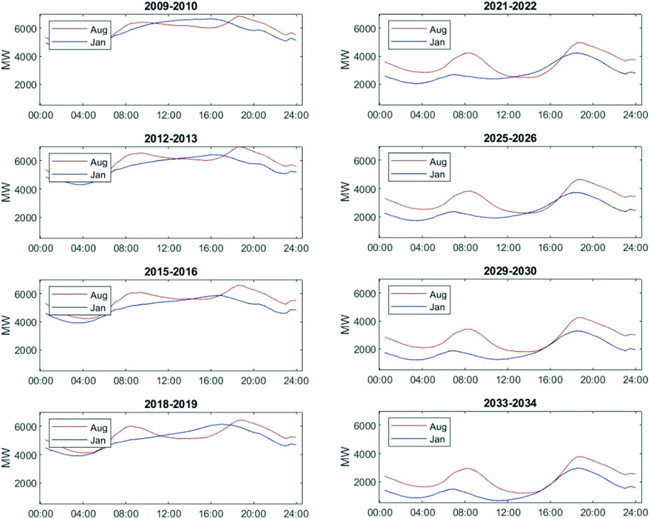
FIGURE 9. The left panel shows intra-day demand patterns in August and January of the first, fourth, seventh, and last financial year of the sample period, i.e., August 2009 and January 2010, August 2012 and January 2013, August 2015 and January 2016, and August 2018 and January 2019. The right panel displays intra-day demand patterns in August and January of the third, seventh, 11th, and last financial year of the forward-looking period, i.e., August 2021 and January 2022, August 2025 and January 2026, August 2029 and January 2030, and August 2033 and January 2034. The half-hourly demand (in MW) is calculated as the average power demand for the same 30-min trading intervals of different days in the corresponding month. The change through time is shown for Victoria.

4.2 Regression results

This section demonstrates the effect of solar generation from rooftop PVs on a half-hourly basis through different regression models, regarding Box 4 in the flow chart of Figure 2. We choose the sample period from 2009 to 2019 to avoid any possible bias arising from the COVID-19 pandemic. We also delete half-hourly observations when there is no rooftop solar generation for five regional markets at the same time, because we are focusing on the periods when generation from small-scale PV systems can make a difference. Some independent variables have a lower frequency, so we use interpolation to make them available on a half-hourly basis. Moreover, it is common to build different models of electricity demand for different states, e.g., the modelling of Al-Musaylh et al. (2018) for Queensland and Ahmed et al. (2012) for NSW.

To rule out the effect of any trends in spot-demand series, we include time passage as a control variable in the model, because the decreasing trend of electricity demand in NSW, SA, Tasmania, and Victoria may affect the results. Moreover, the effect of air temperature on electricity demand is documented in many studies (Apadula et al., 2012; Trotter et al., 2016; Csereklyei et al., 2021). This can arise from the use of energy-draining household appliances, for example if people turn on air conditioning or heating. Heaters will be used more widely in relatively cold areas, being likely to increase power demand if the temperature deviates too much from the level that makes people comfortable, say 18°C. Many socioeconomic variables can also help explain demand deviation from its seasonal trend. Following Hyndman and Fan (2009), Ahmed et al. (2012), and other relevant literature, we consider GSP, state population, the CPI of electricity, and the number of persons per household.

Estimation results in Table 2 confirm that power generation from solar PVs can reduce the deviation of demand from its seasonal patterns in all five states significantly. Based on the full model, a 1 MW increase in rooftop solar generation would reduce around 0.5 MW of spot-demand deviation from its seasonal patterns in Queensland and SA, leading to an even greater impact of more than 0.6 MW in NSW. The last row of Table 2 presents the goodness of fit if the STSCs are added back to the estimated dependent variable. It reaches above 70% in four regional markets, with the exception being SA, where the goodness of fit almost reaches 70%, validating that the model here is well established. Equation 5 is estimated based on data in different half-hourly trading intervals, and the results are shown in Figure 10. The coefficients of rooftop solar generation are quite significant for most of the daytime period. The explanatory power could reach up to 40% in NSW, SA, and Victoria during specific trading intervals, suggesting that rooftop solar has a substantial impact on intra-day patterns of electricity demand, especially in the daytime.

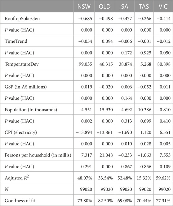
TABLE 2. Results of estimated coefficients in the regression. Dependent variables are the deviation from the seasonal pattern of power demand for five individual states—NSW, Queensland, SA, Tasmania, and Victoria. The explanatory variables are estimates of power generation from rooftop solar, and control variables, including a time trend, temperature deviation from 18°C, GSP, state population, the CPI of electricity, and the number of persons per household. P-Values are based on HAC covariance estimators.

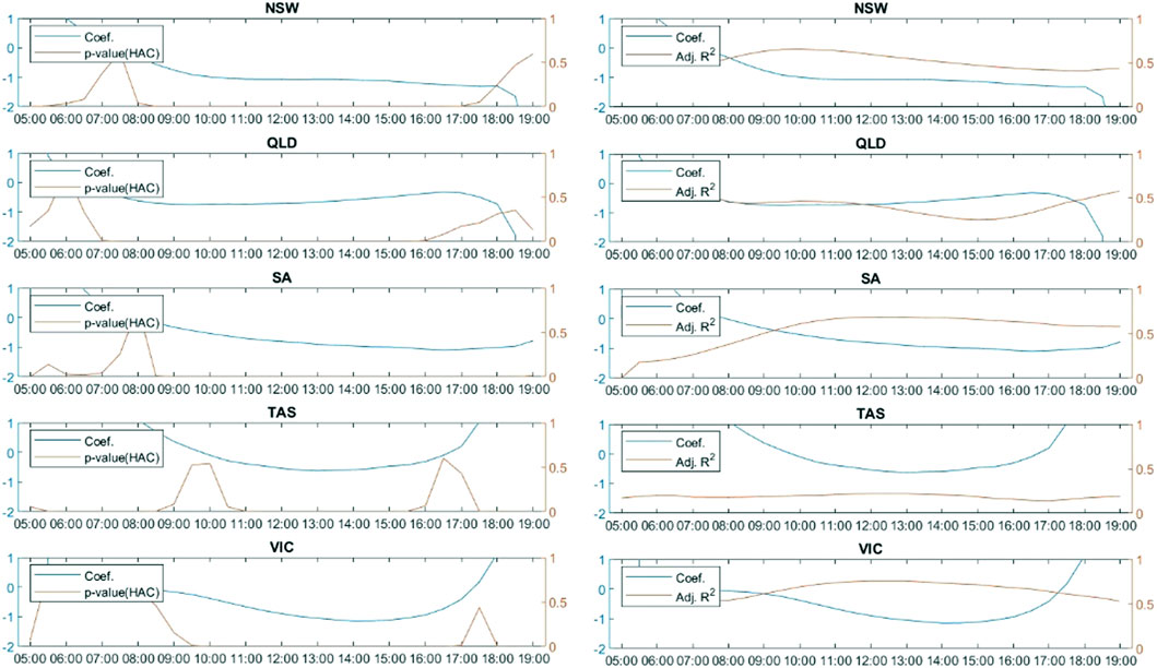
FIGURE 10. Estimation results of the regression model of spot-demand deviation on rooftop solar generation and other control variables, including temperature deviation from 18°C, a time trend, population, GSP, the CPI on electricity, and the number of persons per household. The model is estimated based on data of different half-hourly trading intervals, i.e., 6a.m., 6:30a.m., etc. The left panel presents p-values referring to the probability that the null hypothesis is correct. The null hypothesis is that the coefficient in front of the independent variable equals zero. HAC means the statistics are adjusted in consideration of heteroscedasticity and autocorrelation. The right panel draws adjusted R², which refers to the explanatory power of the model.

Compare with the estimation results of regression models without rooftop solar generation in Supplementary Table A5, we find evidence that solar rooftop plays an important role in explaining the deviation of spot electricity demand from its seasonal patterns. The overall explanatory power of the models without rooftop solar generation as independent variables is relatively lower. Regarding the possible effects of COVID-19, Table 3 suggests that the pandemic does not affect the negative impact of rooftop solar on deseasonalized spot demand in an economically and statistically significant way.

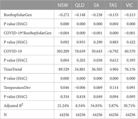
TABLE 3. Estimation results of coefficients in the regression quantifying the impact of COVID-19. Dependent variables are the deviation from the seasonal pattern of power demand for five individual states—NSW, Queensland, SA, Tasmania, and Victoria. The explanatory variables are estimates of power generation from rooftop solar, a dummy indicating the impact of COVID-19, and their cross term. Control variables include a time trend and temperature deviation from 18°C. P-Values are based on HAC covariance estimators.

4.3 Demand forecast for 2019–2034

According to the model built in Section 4.2, we can forecast half-hourly demand from July 2019 onward, which is the goal of Box 7 in the flow chart of Figure 2. Despite actual values being available, we still predict spot demand from July 2019 to June 2022 for two reasons. First, random and temporary events happening to the NEM during this time probably will not have effects in the long term. For example, even though the COVID-19 pandemic has affected patterns of electricity consumption, people’s work and life habits are still expected to go back to normal. Second, the focus of our paper is the effect of rooftop solar, which does not change significantly due to those unpredictable events. Applying estimated coefficients to professional forecasts of explanatory variables in Equation 7, we get deseasonalized spot demand for the five individual states in the NEM. Due to the effects of the COVID-19 pandemic, different STSCs are added back, depending on whether it is before or after the lockdown date of 23 March 2020. Figure 11 and Table 4 show the trend of estimated spot demand from July 2019 to June 2034. On average, spot demand in NSW, Tasmania, and Victoria will keep decreasing after 2019, while Queensland will see spot demand increase for 1 year before the demand declines. Based on our forecast, spot demand in SA will expand gradually after 2 years of falling, which makes it the only state with a different trend.

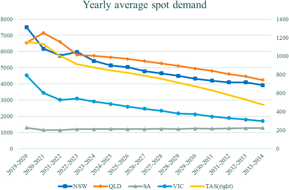
FIGURE 11. Yearly average of forecasted spot demand in megawatts. The values for NSW, Queensland, SA, and Victoria are measured on the left axis while those of Tasmania are shown on the right axis.

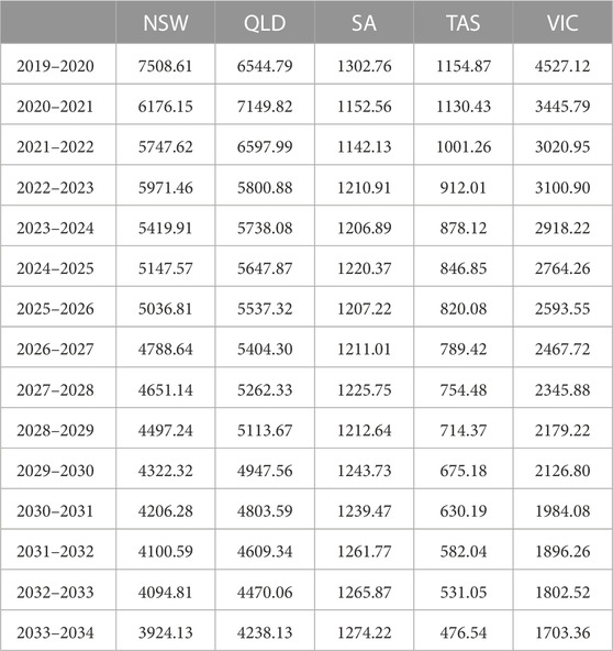
TABLE 4. Yearly average of forecasted spot demand in megawatts.

In the right panels of Figures 5–9, we have also displayed the change to typical intra-day demand patterns due to the effects of rooftop solar under the following assumptions:

1. There will not be significantly massive power storage added to the market during the forecast period.

2. Increasing uptake of electric vehicles (EVs)¹¹ is not considered.

3. Electricity consumption patterns and energy efficiency will not experience significant changes compared with the benchmark period.

The results confirm that total power demand significantly drops for almost every state through the forecasted period, especially in the middle of the daytime, when solar power is more likely to be produced. The concavity in the middle of the intra-day demand pattern becomes lower and lower for both January and August in five states.

In NSW, electricity demand in January was typically highest in the daytime, due to hot weather and the use of air conditioning. This can be obviously seen from intra-day power demand patterns between 2009 and 2019 in the left panel of Figure 5. But according to our forecast, increasing solar power generation from rooftop PVs reduces the load on the grid during daytime in January between 2019 and 2034. The daily highest power demand in January will not be in the middle of the day when it is hottest. Instead, it will be the time when sunshine is not abundant but there is still a need for cooling, usually at dusk.

Similar to the situation in NSW, in Queensland power demand will still increase even after sunrise in the daytime of January between 2009 and 2019. However, forecasted electricity demand starts to go down after sunrise because sunshine can be more efficiently used in the next 15 years thanks to the increasing capacity of rooftop PVs. The intra-day demand pattern in August would also change and the overall level is decreasing. The daily peak of electricity consumption at dusk becomes even more clear.

SA has the highest solar penetration in the NEM, partially replacing fossil fuels with renewables. Its intra-day pattern of spot demand changes more aggressively compared with NSW and Queensland. Due to the application of rooftop solar PVs, electricity demand from the grid drops dramatically after 8a.m., reaching a daily low around 2p.m. that is much lower than any time through the day. It climbs to the daily highest point at about 8p.m., after sunset, and falls afterwards due to people’s declining activity.

Differing from the other four states in the NEM, in the southernmost state of Tasmania, power demand is generally higher in August than in January. There, electricity is consumed more for heating than cooling, especially in winter. Thus, the impact of rooftop solar on half-hourly demand patterns is more profound in August, when the concavity along the corresponding curve is deeper. Apart from that, there is not much variance from the sample period to the next 15 years. The overall demand is decreasing.

Similar to Tasmania, in Victoria, another cooler southern state, the effect of rooftop solar is more prominent in August. There was barely a concavity due to small-scale solar power generation in the daytime along the intra-day demand curve of January—rooftop solar could not significantly reduce electricity demand from the grid before 2020. But the concavity and the daily low along the intra-day power demand curve gradually appear around 12p.m. during the forecast period. Overall, power demand is apparently declining based on our forecast.

To conclude, spot demand will fluctuate considerably during the daytime in the future, which may lead to potential economic losses for coal-fired power plants and also market-wide uncertainty in power supply. In the meantime, uncoordinated charging behavior for an increasing number of EVs may add further uncertainty to the power market. As one solution to this, massive electricity storage could be used to smooth the grid load curve from daytime to nighttime. Alternatively, convenient charging facilities could be installed to encourage people to charge vehicles in the daytime. The situation of uncertainty is likely to worsen if massive storage or coordinated charging behavior does not emerge.

5 Conclusion

This study has analyzed the impact of rooftop solar on demand for power from the electricity grid in the NEM. Based on the novel approach of estimating solar power generation from rooftop PV panels, we have confirmed and quantified the effect of increasing generation capacity from rooftop PV systems. Forecasted spot demand is also provided, given consideration of this profound effect.

To conclude, we find that:

1. Rooftop solar generation has significantly reduced the total market load for the NSW, SA, and Victoria regions over time.

2. Increasing rooftop solar power generation has changed the intra-day patterns of power demand. Its effect is clearer during half-hourly trading intervals in the daytime.

3. A 1 MW increase in rooftop solar generation would subtract more than 0.6 MW of spot-demand deviation from its seasonal patterns in NSW. The reduction caused by 1 MW of added rooftop solar generation reaches about 0.5 MW in Queensland, SA, and Victoria.

4. The COVID-19 pandemic does not affect the impact of rooftop solar on deseasonalized spot demand significantly.

5. The forecasted demand suggests obvious declining trends in four regional markets, namely NSW, Queensland, Tasmania, and Victoria, while overall spot demand grows after a few years’ decline in SA.

6. Due to the growth of solar power generation from rooftop PVs, the peak of intra-day electricity consumption will gradually move from midday to dusk in the near future.

Compared with the results of Mwampashi et al. (2022) whose research setting is similar to us, we both find that the high uptake of rooftop solar PVs can make more power available in the daytime, pushing the electricity consumption peak towards early evening hours. The difference is that we also provide demand forecast for 15 years in addition to analyzing and modelling the impact of solar rooftop.

There are also some uncertainties and limitations of our study. First, other variables that may affect electricity spot demand could be omitted in the built regression models, which would impair the accuracy of our results. Second, there are uncertainties regarding climate change itself as well as the corresponding adaption and mitigation measures. These uncertainties could change the relationships drawn from current datasets. For example, wide-range deployment of home battery storage increases the efficiency of utilizing rooftop solar energy, which would lead to intra-day transfer of electricity consumption. Last but not least, as the focus of our paper is the impact of solar rooftop rather than electricity demand forecast, we do not apply AI-based methods despite their outstanding performances. Future research could take into account the structural changes in energy markets, such as the increase in renewables, EV, and energy efficiency, when employing the forecasting techniques based on deep learning.

Data availability statement

The original contributions presented in the study are included in the article/Supplementary Material, further inquiries can be directed to the corresponding author.

Author contributions

GY and LH contributed to conception and design of the study. GY organized the database, performed the statistical analysis, wrote the first draft of the manuscript, and made revisions. LH wrote one subsection of the manuscript. All authors contributed to the article and approved the submitted version.

Funding

GY appreciates the funding support by China Postdoctoral Science Foundation (Grant No. 2022M710009).

Conflict of interest

The authors declare that the research was conducted in the absence of any commercial or financial relationships that could be construed as a potential conflict of interest.

Publisher’s note

All claims expressed in this article are solely those of the authors and do not necessarily represent those of their affiliated organizations, or those of the publisher, the editors and the reviewers. Any product that may be evaluated in this article, or claim that may be made by its manufacturer, is not guaranteed or endorsed by the publisher.

Supplementary material

The Supplementary Material for this article can be found online at: https://www.frontiersin.org/articles/10.3389/fenrg.2023.1197504/full#supplementary-material

Footnotes

¹It is referred to as the merit order effect. See Bell et al. (2017) for a review concerning the merit order effect from different countries using different methodologies.

²Utility-scale VRE generation increases the supply of low-cost power, while rooftop solar power reduces demand for the electricity that needs to be supplied through the grid. They affect electricity markets in different ways.

³There are three types of estimates in the AEMO’s model: daily, measurement, and satellite. Subject to availability, we always choose the estimate of the best quality, whose indicator equals 1 in most cases.

⁴Detailed instructions on data usage are on the Clean Energy Regulator website, http://www.cleanenergyregulator.gov.au/RET/Forms-and-resources/Postcode-data-for-small-scale-installations.

⁵Detailed results of the estimated seasonal component are not provided here, but are available from the authors on request.

⁶For example, to simulate a block starting on 1 June 2023 with a length of 3 days, the days from 15 April 2009 to 15 July 2009, from 15 April 2010 to 15 July 2010, from 15 April 2011 to 15 July 2011, etc., will be used as the sampling period to bootstrap from.

⁷Seasonal patterns are subtracted from spot demand. It is for investigating more clearly whether and how demand can be explained by increasing adoption of rooftop solar PV systems, reducing the effect of people’s energy-consumption habits.

⁸The estimates from July 2009 to July 2016 are based on the methodology introduced in Section 2.1. We adopt the AEMO estimates from August 2016 on.

⁹We subtract seasonal patterns from demand to investigate more clearly whether and how demand can be explained by increasing adoption of rooftop solar PV systems, reducing the effect of people’s energy-consumption habits.

¹⁰We have also calculated the results under the most likely scenario, “step change”. The difference from those shown in the paper is trivial. These results are available from the authors upon request.

¹¹The results, considering forecasted EV charging patterns, are shown in Supplementary Figures A4, A5. Adopted estimation methods are available from the authors on request. The projection of EV numbers, estimated charging types, and the corresponding charging patterns, is from the Australian Energy Market Operator (2022). We do not discuss the results here in detail because the effects of EVs are trivial until 2030.

References

Ahmed, T., Muttaqi, K., and Agalgaonkar, A. (2012). Climate change impacts on electricity demand in the state of new South wales, Australia. Appl. Energy98, 376–383. doi:10.1016/j.apenergy.2012.03.059
Al Khafaf, N., Rezaei, A. A., Amani, A. M., Jalili, M., McGrath, B., Meegahapola, L., et al. (2022). Impact of battery storage on residential energy consumption: An Australian case study based on smart meter data. Renew. Energy182, 390–400. doi:10.1016/j.renene.2021.10.005
Al Mamun, A., Sohel, M., Mohammad, N., Sunny, M. S. H., Dipta, D. R., and Hossain, E. (2020). A comprehensive review of the load forecasting techniques using single and hybrid predictive models. IEEE Access8, 134911–134939. doi:10.1109/access.2020.3010702
Al-Musaylh, M. S., Deo, R. C., Adamowski, J. F., and Li, Y. (2018). Short-term electricity demand forecasting with MARS, SVR and ARIMA models using aggregated demand data in Queensland, Australia. Adv. Eng. Inf.35, 1–16. doi:10.1016/j.aei.2017.11.002
Alrawi, O. F., Al-Siddiqi, T., Al-Muhannadi, A., Al-Siddiqi, A., and Al-Ghamdi, S. G. (2022). Determining the influencing factors in the residential rooftop solar photovoltaic systems adoption: Evidence from a survey in Qatar. Energy Rep.8, 257–262. doi:10.1016/j.egyr.2022.01.064
Alsaedi, Y., Tularam, G. A., and Wong, V. (2020). Assessing the effects of solar and wind prices on the Australia electricity spot and options markets using a vector autoregression analysis. Int. J. Energy Econ. Policy10 (1), 120–133. doi:10.32479/ijeep.8567
Aneiros, G., Vilar, J., and Raña, P. (2016). Short-term forecast of daily curves of electricity demand and price. Int. J. Electr. Power & Energy Syst.80, 96–108. doi:10.1016/j.ijepes.2016.01.034
Apadula, F., Bassini, A., Elli, A., and Scapin, S. (2012). Relationships between meteorological variables and monthly electricity demand. Appl. Energy98, 346–356. doi:10.1016/j.apenergy.2012.03.053
Australian Energy Market Operator (2022). 2022 integrated system plan for the National Electricity Market [online]. Available at: https://aemo.com.au/energy-systems/major-publications/integrated-system-plan-isp/2022-integrated-system-plan-isp (Released June 2, 2022).
Australian Energy Market Operator, 2021. State of the energy market 2021 [online]. Released 2 July, 2021, Available at: https://www.aer.gov.au/publications/state-of-the-energy-market-reports/state-of-the-energy-market-2021.
Australian Energy Market Operator, Energy Networks Australia (2019). Open energy networks: Required capabilities and recommended actions [online]. Released on Available at: https://www.energynetworks.com.au/projects/open-energy-networks.
Bell, W. P., Wild, P., Foster, J., and Hewson, M. (2017). Revitalising the wind power induced merit order effect to reduce wholesale and retail electricity prices in Australia. Energy Econ.67, 224–241. doi:10.1016/j.eneco.2017.08.003
Bierbrauer, M., Menn, C., Rachev, S., and Trück, S. (2007). Spot and derivative pricing in the EEX power market. J. Bank. Finance31, 3462–3485. doi:10.1016/j.jbankfin.2007.04.011
Blakers, A., Stocks, M., Lu, B., and Cheng, C. (2021). The observed cost of high penetration solar and wind electricity. Energy233, 121150. doi:10.1016/j.energy.2021.121150
Cardenas, L., Zapata, M., Franco, C. J., and Dyner, I. (2017). Assessing the combined effect of the diffusion of solar rooftop generation, energy conservation and efficient appliances in households. J. Clean. Prod.162, 491–503. doi:10.1016/j.jclepro.2017.06.068
Collier, S. H., House, J. I., Connor, P. M., and Harris, R. (2023). Distributed local energy: Assessing the determinants of domestic-scale solar photovoltaic uptake at the local level across England and Wales. Renew. Sustain. Energy Rev.171, 113036. doi:10.1016/j.rser.2022.113036
Csereklyei, Z., Qu, S., and Ancev, T. (2021). Are electricity system outages and the generation mix related? Evidence from NSW, Australia. Energy Econ.99, 105274. doi:10.1016/j.eneco.2021.105274
Csereklyei, Z., Qu, S., and Ancev, T. (2019). The effect of wind and solar power generation on wholesale electricity prices in Australia. Energy Policy131, 358–369. doi:10.1016/j.enpol.2019.04.007
Earle, L., Maguire, J., Munankarmi, P., and Roberts, D. (2023). The impact of energy-efficiency upgrades and other distributed energy resources on a residential neighborhood-scale electrification retrofit. Appl. Energy329, 120256. doi:10.1016/j.apenergy.2022.120256
El-Adaway, I. H., Sims, C., Eid, M. S., Liu, Y., and Ali, G. G. (2020). Preliminary attempt toward better understanding the impact of distributed energy generation: An agent-based computational economics approach. J. Infrastructure Syst.26 (1), 04020002. doi:10.1061/(asce)is.1943-555x.0000527
Franco, G., and Sanstad, A. H. (2008). Climate change and electricity demand in California. Clim. Change87 (1), 139–151. doi:10.1007/s10584-007-9364-y
Geman, H., and Roncoroni, A. (2006). Understanding the fine structure of electricity prices. J. Bus.79 (3), 1225–1261. doi:10.1086/500675
Gonçalves, R., and Menezes, F. (2022). Market-wide impact of renewables on electricity prices in Australia. Econ. Rec.98 (320), 1–21. doi:10.1111/1475-4932.12642
Higgs, H., Lien, G., and Worthington, A. C. (2015). Australian evidence on the role of interregional flows, production capacity, and generation mix in wholesale electricity prices and price volatility. Econ. Analysis Policy48, 172–181. doi:10.1016/j.eap.2015.11.008
Hsiao, Y.-H. (2014). Household electricity demand forecast based on context information and user daily schedule analysis from meter data. IEEE Trans. Industrial Inf.11 (1), 33–43. doi:10.1109/tii.2014.2363584
Hyndman, R. J., and Fan, S. (2009). Density forecasting for long-term peak electricity demand. IEEE Trans. Power Syst.25 (2), 1142–1153. doi:10.1109/tpwrs.2009.2036017
Janczura, J., Trück, S., Weron, R., and Wolff, R. C. (2013). Identifying spikes and seasonal components in electricity spot price data: A guide to robust modeling. Energy Econ.38, 96–110. doi:10.1016/j.eneco.2013.03.013
Laker, I., Huang, C.-K., and Clark, A. E. (2017). Dependent bootstrapping for value-at-risk and expected shortfall. Risk Manag.19 (4), 301–322. doi:10.1057/s41283-017-0023-y
Lindberg, K., Seljom, P., Madsen, H., Fischer, D., and Korpås, M. (2019). Long-term electricity load forecasting: Current and future trends. Util. Policy58, 102–119. doi:10.1016/j.jup.2019.04.001
López Prol, J., Steininger, K. W., and Zilberman, D. (2020). The cannibalization effect of wind and solar in the California wholesale electricity market. Energy Econ.85, 104552. doi:10.1016/j.eneco.2019.104552
McFarland, J., Zhou, Y., Clarke, L., Sullivan, P., Colman, J., Jaglom, W. S., et al. (2015). Impacts of rising air temperatures and emissions mitigation on electricity demand and supply in the United States: A multi-model comparison. Clim. Change131 (1), 111–125. doi:10.1007/s10584-015-1380-8
Morcillo, J., Castaneda, M., Jímenez, M., Zapata, S., Dyner, I., and Aristizabal, A. J. (2022). Assessing the speed, extent, and impact of the diffusion of solar PV. Energy Rep.8, 269–281. doi:10.1016/j.egyr.2022.06.099
Mwampashi, M. M., Nikitopoulos, C. S., Rai, A., Konstandatos, O., and 11, (2022). Large-scale and rooftop solar generation in the NEM: A tale of two renewables strategies. Energy Econ.115, 106372. doi:10.1016/j.eneco.2022.106372
Nti, I. K., Teimeh, M., Nyarko-Boateng, O., and Adekoya, A. F. (2020). Electricity load forecasting: A systematic review. J. Electr. Syst. Inf. Technol.7 (1), 13–19. doi:10.1186/s43067-020-00021-8
O’Shaughnessy, E., Barbose, G., Wiser, R., Forrester, S., and Darghouth, N. (2021). The impact of policies and business models on income equity in rooftop solar adoption. Nat. Energy6 (1), 84–91. doi:10.1038/s41560-020-00724-2
Patton, A., Politis, D. N., and White, H. (2009). Correction to “Automatic block-length selection for the dependent bootstrap” by D. Politis and H. White. Econ. Rev.28 (4), 372–375. doi:10.1080/07474930802459016
Perez-Arriaga, I. J. (2016). The transmission of the future: The impact of distributed energy resources on the network. IEEE Power Energy Mag.14 (4), 41–53. doi:10.1109/mpe.2016.2550398
Politis, D. N., and Romano, J. P. (1994). The stationary bootstrap. J. Am. Stat. Assoc.89 (428), 1303–1313. doi:10.1080/01621459.1994.10476870
Politis, D. N., and White, H. (2004). Automatic block-length selection for the dependent bootstrap. Econ. Rev.23 (1), 53–70. doi:10.1081/etc-120028836
Quint, R., Dangelmaier, L., Green, I., Edelson, D., Ganugula, V., Kaneshiro, R., et al. (2019). Transformation of the grid: The impact of distributed energy resources on bulk power systems. IEEE Power Energy Mag.17 (6), 35–45. doi:10.1109/mpe.2019.2933071
Rai, A., and Nunn, O. (2020). On the impact of increasing penetration of variable renewables on electricity spot price extremes in Australia. Econ. analysis policy67, 67–86. doi:10.1016/j.eap.2020.06.001
Ros, A. J., and Sai, S. S. (2023). Residential rooftop solar demand in the US and the impact of net energy metering and electricity prices. Energy Econ.118, 106491. doi:10.1016/j.eneco.2022.106491
Sensfuß, F., Ragwitz, M., and Genoese, M. (2008). The merit-order effect: A detailed analysis of the price effect of renewable electricity generation on spot market prices in Germany. Energy Policy36 (8), 3086–3094. doi:10.1016/j.enpol.2008.03.035
Shaw-Williams, D., Susilawati, C., Walker, G., and Varendorff, J. (2019). Valuing the impact of residential photovoltaics and batteries on network electricity losses: An Australian case study. Util. Policy60, 100955. doi:10.1016/j.jup.2019.100955
Shen, X., Qiu, Y. L., Bo, X., Patwardhan, A., Hultman, N., and Dong, B. (2023). The impact of co-adopting electric vehicles, solar photovoltaics, and battery storage on electricity consumption patterns: Empirical evidence from Arizona. Resour. Conservation Recycl.192, 106914. doi:10.1016/j.resconrec.2023.106914
Simshauser, P., and Akimov, A. (2019). Regulated electricity networks, investment mistakes in retrospect and stranded assets under uncertainty. Energy Econ.81, 117–133. doi:10.1016/j.eneco.2019.03.027
Simshauser, P. (2022). Rooftop solar PV and the peak load problem in the NEM’s Queensland region. Energy Econ.109, 106002. doi:10.1016/j.eneco.2022.106002
Srianandarajah, N., Wilson, S. J., and Chapman, A. C. (2022). From green to amber: Is Australia’s national electricity market signalling a financial warning for wind and solar power?Energy Policy167, 113052. doi:10.1016/j.enpol.2022.113052
Trotter, I. M., Bolkesjø, T. F., Féres, J. G., and Hollanda, L. (2016). Climate change and electricity demand in Brazil: A stochastic approach. Energy102, 596–604. doi:10.1016/j.energy.2016.02.120
Vanting, N. B., Ma, Z., and Jørgensen, B. N. (2021). A scoping review of deep neural networks for electric load forecasting. Energy Inf.4, 49–13. doi:10.1186/s42162-021-00148-6
Weron, R. (2006). Modeling and forecasting loads and prices in deregulated electricity markets. Chichester: Wiley.
Wilkinson, S., Maticka, M. J., Liu, Y., and John, M. (2021). The duck curve in a drying pond: The impact of rooftop PV on the Western Australian electricity market transition. Util. Policy71, 101232. doi:10.1016/j.jup.2021.101232
Wu, J., Levi, N., Araujo, R., and Wang, Y.-G. (2023). An evaluation of the impact of Covid-19 lockdowns on electricity demand. Electr. Power Syst. Res.216, 109015. doi:10.1016/j.epsr.2022.109015
Yan, G., and Trück, S. (2020). A dynamic network analysis of spot electricity prices in the Australian national electricity market. Energy Econ.92, 104972. doi:10.1016/j.eneco.2020.104972
Zander, K. K., Simpson, G., Mathew, S., Nepal, R., and Garnett, S. T. (2019). Preferences for and potential impacts of financial incentives to install residential rooftop solar photovoltaic systems in Australia. J. Clean. Prod.230, 328–338. doi:10.1016/j.jclepro.2019.05.133
Keywords: solar energy, energy transition, spot electricity demand, rooftop PV, renewable energy
Citation: Yan G and Han L (2023) The impact of rooftop solar on wholesale electricity demand in the Australian National Electricity Market. Front. Energy Res. 11:1197504. doi: 10.3389/fenrg.2023.1197504
Received: 03 April 2023; Accepted: 07 June 2023;
Published: 26 June 2023.
Edited by:
Nallapaneni Manoj Kumar, City University of Hong Kong, Hong Kong SAR, ChinaReviewed by:
Sonali Goel, Independent Researcher, Bhubaneswar, IndiaNeeraj Kumar Singh, NeST Digital, India
Copyright © 2023 Yan and Han. This is an open-access article distributed under the terms of the Creative Commons Attribution License (CC BY). The use, distribution or reproduction in other forums is permitted, provided the original author(s) and the copyright owner(s) are credited and that the original publication in this journal is cited, in accordance with accepted academic practice. No use, distribution or reproduction is permitted which does not comply with these terms.
*Correspondence: Guan Yan, yanguan@ustb.edu.cn