Unmanned Aerial Vehicle (UAV)-Based Thermal Infra-Red (TIR) and Optical Imagery Reveals Multi-Spatial Scale Controls of Cold-Water Areas Over a Groundwater-Dominated Riverscape
 Roser Casas-Mulet
 Joachim Pander
 Dongryeol Ryu
 Michael J. Stewardson
 Juergen Geist
- 1Aquatic Systems Biology Unit, School of Life Sciences Weihenstephan, Technical University of Munich, Freising, Germany
- 2Department of Infrastructure Engineering, School of Engineering, University of Melbourne, Melbourne, VIC, Australia
- 3Water Research Institute, Cardiff University, Cardiff, United Kingdom
The forecast of warmer weather, and reduced precipitation and streamflow under climate change makes freshwater biota particularly vulnerable to being exposed to temperature extremes. Given the importance of temperature to regulate vital physiological processes, the availability of discrete cold-water patches (CWPs) in rivers to act as potential thermal refugia is critical to support freshwater ecosystem function. Being able to predict their spatial distribution at riverscape scales is the first step to understanding the capacity to maintain thermal refuges and to inform future river management strategies. Novel Unmanned Aerial Vehicle (UAV)-based Thermal Infra-Red (TIR) imagery technologies provide an opportunity to assess riverscape stream temperature. On the example of a 50 km linear length of the groundwater-dominated Upper Ovens River (Australia), this study presents a methodology addressing critical challenges in UAV-based TIR and optical data acquisition, processing, and interpretation. Our methodological approach generated 49 georeferenced high-resolution TIR and optical orthomosaicked imagery sets. The imagery sets allowed us to identify river-length longitudinal patterns of temperature and to detect, characterize, and classify 260 CWPs. Both stream and CWPs temperatures increased but presented considerable variability with downstream distance. CWPs were non-uniformly distributed along the riverscape, with emergent hyporheic water types dominating, followed by deep pools, shading, side channels, and tributaries. We found associations between CWPs and key physical controls including land use, riparian vegetation, longitudinal and lateral CWP location, and CWP area size, illustrating processes acting at multiple spatial scales. This study provides a basis for future works on the thermal associations with physical controls over a riverscape, and it highlights the major challenges and limitations of the use of UAV-based TIR and optical imagery to be used in future applications. In conjunction with studies of thermally linked ecological processes, the predictions of CWPs can help prioritize river restoration measures as effective climate adaptation tools.
Introduction
The forecast of continued durations of warmer weather, altered precipitation, and modified streamflow patterns driven by climate change will be exacerbated by local anthropogenic pressures in rivers, exposing freshwater ecosystems to a severe threat worldwide (Vörösmarty et al., 2010; Reid et al., 2019). Land-use change, water abstractions, and stream regulation pose severe alterations to rivers, with increased drought severity, high stream temperatures and habitat degradation of most concern (Bond et al., 2008; van Vliet et al., 2013; Geist and Hawkins, 2016). Such unprecedented changes in aquatic systems call for action to develop effective management and mitigation approaches to support river resilience (Palmer et al., 2008; Wilby et al., 2010; McCluney et al., 2014).
As river temperatures are expected to increase globally (Kaushal et al., 2010; van Vliet et al., 2013; Orr et al., 2015), cold-water thermal refugia are increasingly considered as a targeted climate adaptation strategy in the northern hemisphere (Kurylyk et al., 2014; Isaak et al., 2015). Adapted from the definition of climatic refuges by James et al. (2013), here we consider thermal refuges as discrete patches of water at either lower or higher temperature than the main stream, in which biota can persist during periods of unfavorable thermal conditions. Here, we will focus on cold-water patches (CWPs), most relevant as potential thermal refuges during summer. Based on the recognition that stream temperature is the “master” variable controlling biochemical processes in rivers (Caissie, 2006; Webb et al., 2008), thermal refuges need to be incorporated as a key aspect of river habitat structure, and to be considered in freshwater climate adaptation management strategies around the world (Palmer et al., 2008; Keppel et al., 2015; Morelli et al., 2016).
Rivers are complex dynamic ecosystems that vary significantly along their spatial course (Wohl, 2016). Their physical structure can be represented as a hierarchical organization of interconnected spatial scales (Frissell et al., 1986; Thorp et al., 2006; Braun et al., 2012). Such array of physical features play an essential role in determining how heat is distributed (Fausch et al., 2002; Carbonneau et al., 2012). Whilst river temperature is driven by climatic, topographic, and hydrological controls at the air-water interface (Caissie, 2006; Webb et al., 2008); dynamic groundwater inputs (Poole et al., 2006; Arrigoni et al., 2008; Dugdale et al., 2013), in-channel physical complexity (Tonolla et al., 2010; Sawyer and Cardenas, 2012), and shading (Torgersen et al., 1999; Garner et al., 2017) may alter its longitudinal variability. Understanding the spatial variations of stream temperature and the processes governing CWPs within the riverscape is of key concern for managers (Kurylyk et al., 2014; Steel et al., 2017). Whilst the spatial distribution of CWPs was earlier considered by Ebersole et al. (2003b) and Torgersen et al. (1999), recent technological advances in Thermal Infra-Red (TIR) imagery acquisition have propelled investigations of their driving processes at larger spatial scales including entire riverscapes (Handcock et al., 2012; Dugdale, 2016; Dugdale et al., 2019). Monk et al. (2013), for example, demonstrated the links between a range of physical environmental variables and cold-tributary areas using TIR imagery coupled with geospatial landscape information over a reach of the Cains River in Canada. Dugdale et al. (2015), on the other hand, studied the spatial variability of groundwater-based cold-water refuges and their associations with watershed hydromorphology combining TIR and optical imagery in the Restigouche River, Canada. Both TIR and optical imagery were also used along a ca. 50 km river length of the Ain River, in France, to (i) find that CWPs were associated to fluvial geomorphic features (Wawrzyniak et al., 2016); and (ii) demonstrate TIR mapping efficiency to detect groundwater-driven cold upwellings (Dole-Olivier et al., 2019). Whilst the clear effect of controls such as riparian shading, land use and in-channel fluvial geomorphology on stream temperature has been demonstrated (e.g., land use, Allan, 2004; riparian shading, Ebersole et al., 2003a; Garner et al., 2017; geomorphic features, Ouellet et al., 2017), studies of their combined influence over large spatial scales are rare. The incorporation of such key mechanisms into integrated predictive models of thermal refuge distribution will be key to understand and manage future climatic conditions (Fullerton et al., 2018).
Recent advances in the development of UAVs – or drones – equipped with TIR cameras provide small, inexpensive, fast, and flexible solutions to obtain high-resolution TIR and optical (RGB) imagery data (Corti Meneses et al., 2018a, b). UAVs are also capable of surveying large areas that, to date, were primarily carried out using manned aerial vehicles (i.e., helicopter). The use of light-weight uncooled thermal cameras in drones, however, comes with some limitations including sensor and environmentally derived errors (Dugdale et al., 2019; Kelly et al., 2019), and the difficulty in orthomosaicking in the photogrammetric process due to the inherent low contrast of surface features in TIR images (Ribeiro-Gomes et al., 2017). To address these and other issues affecting TIR imagery quality, it is crucial to develop a functional methodology during data acquisition and processing that helps obtain high precision quantitative stream temperature information for its correct interpretation.
To date, most literature on the identification, distribution and use of cold-water refuges is found in the northern hemisphere, focusing in particular on their role to aid salmonids’ thermoregulation during hot extremes (Ebersole et al., 2001; McCullough et al., 2009). In contrast, in the southern hemisphere, in south-eastern Australia, significant research progress has been made in understanding flow-associated “climatic” or “drought” refuges (Bond, 2007; James et al., 2013; Robson et al., 2013; Ning et al., 2015), driven by the predicted increased recurrence of droughts due to climate change (Boulton, 2003; Murray-Darling Basin Commission, 2007; Bond et al., 2008). However, such research progress has focused on ephemeral or near-ephemeral streams, leaving an open gap on stream thermal refuge research in perennial rivers in Australia.
The perennial Upper Ovens River (Victoria, Australia) is one of the least modified catchments within the Murray-Darling Basin (Miller and Barbee, 2003). It supports high ecological values due to its distinctly connected surface and groundwater sources (Yu et al., 2013). However, future climatic predictions will make it extremely vulnerable during summer low flows, as the heightened anthropogenic groundwater extractions are likely to create cease-to-flow events with high risk to freshwater biota (Goulburn Murray Water, 2011). Since 2008, the Upper Ovens River has been declared a Water Supply Protection Area, with a priority goal to reduce the risk of aquatic habitat loss during critical low flow periods, by restricting water demands when necessary (Goulburn Murray Water, 2011; Hart and Doolan, 2017). Identifying and understanding the capacity of the system to hold thermal refuges is therefore essential to enable the implementation of well-informed and targeted restrictions, and to support long-term climate adaption and mitigation strategies in the system.
To tackle the above-mentioned gaps, this study takes the Upper Ovens River as a riverscape model to (i) present a methodology addressing the key challenges during UAV-based TIR and optical imagery acquisition, processing and interpretation; (ii) investigate patterns of riverscape stream temperature and CWPs, and (iii) model the associations of CWPs with physical controls at multiple spatial scales. We also discuss the implications of the findings in the context of freshwater conservation and management.
Materials and Methods
The Upper Ovens River
The Upper Ovens River (Australia) is part of a vast anabranching system across the south-east Murray-Darling Basin (Figure 1) that emerges from the northern part of the Victorian Alps and flows north-westwards (Judd et al., 2007). With a steep surface gradient, the Upper Ovens River presents a variety of landscapes ranging from narrow V-shaped mountain valley forming a single channel, covered by native forests and extensive pine forestry plantations, to a broad flat alluvial floodplain with a meandering multi-channel river, surrounded predominately by agricultural land (Sinclair Knight Merz, 2013).
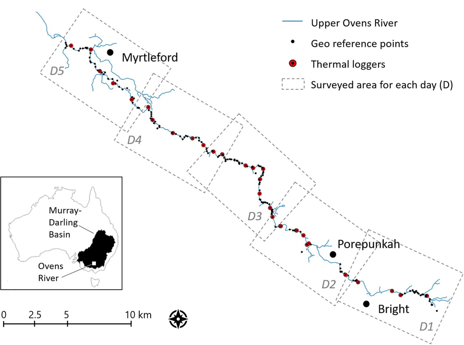
Figure 1. Location of the Upper Ovens River with the position of all Ground Control Points (GCPs) and thermal references, and the delimitation of the areas surveyed each day (D).
The average annual rainfall in the Upper Ovens is 1000 mm, with a monthly average between 57 mm in February and 181 mm in July. These result in seasonal stream water level fluctuations of up to 2 m with the highest levels coinciding with maximum peak spring rainfall (Sinclair Knight Merz, 2007).
The geology of the Upper Ovens catchment is characterized by ancestral incision into Ordovician bedrock, which was infilled by alluvial deposits comprising the deeper, coarse-grained Calivil Formation; shallower sands, silts, and clays of the Shepparton Formation; and the recent alluvium of the Coonambidgal Formation (Shugg, unpublished). Groundwater flows both regionally in the Ordovician fractured rock aquifer and locally in the alluvial sediments in the valley. The river and floodplain were dredged over the last 150 years to mine gold. The dredging process involved significant disturbance of shallow sediments by successive excavation, mixing, re-constitution, and re-deposition resulting in substantial changes in stream morphology (Sinclair Knight Merz, 2007).
The Upper Ovens River flows to the northwest, dominated by gaining reaches consistent with topography and aquifer lithology. Groundwater constitutes most of the river flow during baseflow conditions in summer, with total groundwater inflow increasing with river flow. Estimates of the contribution of groundwater to the total flow vary greatly depending on the method but are considered higher in the Upper Ovens River compared to other parts of the catchment (Yu et al., 2013). Rapid groundwater recharge through the permeable aquifers rises the water table. In turn, the hydraulic head gradient toward the river increases and hence causes high baseflow to the river during high flow (wet) periods (Yu et al., 2013). Surface water and groundwater extraction, and change in land use (such as clearing, re-afforestation, or increasing irrigation) can influence the volume of groundwater discharging to the river (Owuor et al., 2016). During summer months, when flows are at their minimum but demand for surface and groundwater are at their highest, the Upper Ovens River experiences significant water stress (Goulburn Murray Water, 2011; Yu et al., 2013).
Methodological Approach
A combination of ground data collection and desktop works are usually required for the acquisition, calibration, correction, orthomosaick stitching, and interpretation of airborne imagery. In this study, we applied a step-by-step approach subdivided into three phases comprising data acquisition, processing, and interpretation (Figure 1). In summary, we deployed ground control points (GCPs) and thermal loggers for calibration/validation along the survey area, and we measured them before dual UAV-based flights for thermal and optical imagery data acquisition were carried out. Desktop-based processing encompassed thermal calibration via linear models; temperature drift correction using Partially Overlapped Histogram Equalization (POHE); imagery georeferencing; raster photogrammetric orthomosaicking; georectification; longitudinal temperature adjustment; and thermal validation using temperature logger data. As part of data interpretation, orthomosaicked raster TIR images were polygonized to help CWPs identification based on established thermal thresholds; both physical and thermal attributes were extracted from optical, and TIR imagery, respectively; and the overlapping of both imagery provided the basis of CWPs classification.
Data Acquisition
Field data acquisition via UAV-based TIR and optical (RGB) imagery took place over five consecutive days with stable warm summer weather conditions (2–7 April 2017), and low flows in the Upper Ovens River (2.4 ± 0.17 m3.s–1, Myrtleford station, Australian Government Bureau of Meteorology, 2018). We covered 7–10 km of linear distance per day including the river length from above Bright to below Myrtleford (50 km in linear length, and ca 95 km in total river length).
Each day, prior to the UAV-surveys, a total of 40–60 GCPs were distributed along the planned surveyed area (Figure 1), and their location was recorded using Leica® Viva GS14 RTK differential global positioning system (DGPS), for georectification (Figure 2). They consisted of a combination of cold and warm targets to enable their detection by TIR images. The targets were made of 50 × 50 cm metallic sheets (cold) and rubber tiles (warm) marked with a “ + ” in the middle. We located them in non-vegetated riparian areas or on exposed gravel bars to enable easy visualization from the air, and we retrieved them at the end of each daily survey. A total of 31 Cyclops® temperature loggers were distributed along the surveyed river length for thermal validation over the water target (Figure 1). Five to seven loggers were installed across the planned surveyed area prior to the UAV flights, geo-located with DGPS, and retrieved at the end of the day with the time series of water temperature over the flight duration. They were installed approximately 5 cm below the water surface with the aid of a metallic stack located in the river thalweg, and recorded temperatures at 10 min intervals. The logger located further downstream each day was left in the river for the next day survey to enable modeling of temperatures at all logger locations.
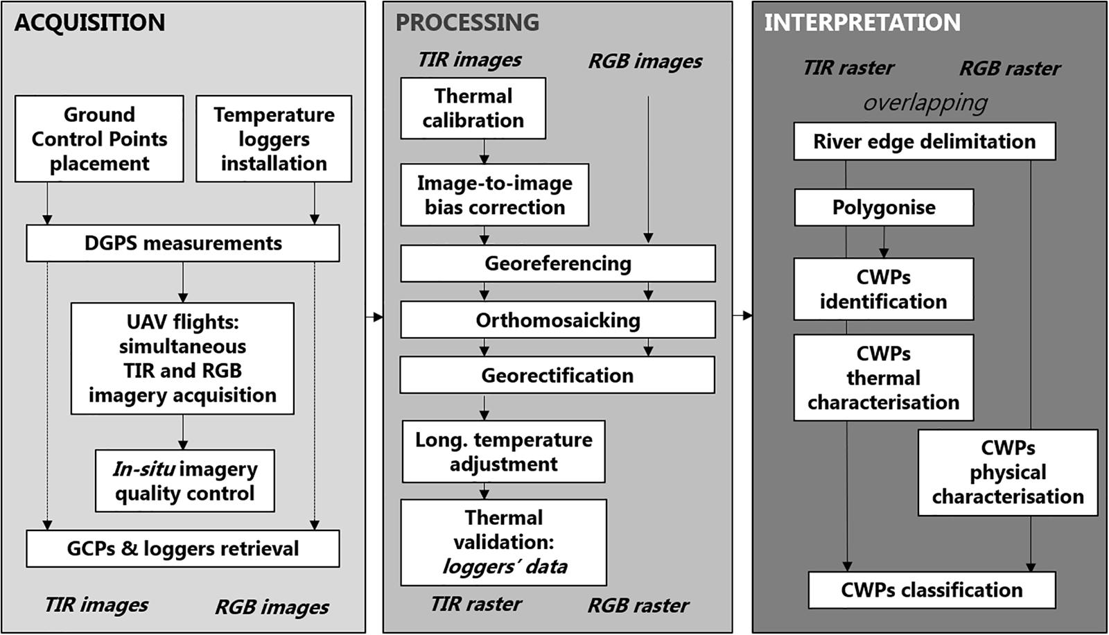
Figure 2. Diagram of the methodological approach for UAV-based TIR and optical (RGB) imagery data acquisition, processing, and interpretation.
We used two drones (Phantom 4 Pro and DJI Inspire 1 Pro of DJI) to collect close-to-nadir optical and TIR imagery simultaneously. Phantom 4 Pro was used to carry a Zenmuse X5 RGB camera to acquire optical photos; and Inspire 1 Pro a Zenmuse XT-Radiometric thermal camera (640 × 512 pixels), with 13 mm wide lenses, for TIR imagery acquisition. We used 23 bases along the surveyed length from which we took off a total of 49 paired flights. Flights were carried out between 12:00 and 14:00 h each day, when the sun reaches its highest position, to allow higher air-water thermal contrast and less shading effect (Dugdale et al., 2015). Some earlier (11:00 h) and later (15:30 h) flights were taken to maximize the daily flight time. They were considered suitable for the detection of thermal differences as continuous logging devices revealed minimum changes in stream temperature within these time thresholds. Besides, in situ imagery checks revealed no major differences in stream temperature between these and later or earlier flights. At each base, two professional drone pilots carried out the flights. The use of professional drone pilots was required to comply with the strict Civil Aviation Safety Authority (CASA) regulations in Australia, given that the total drone payload was over 2 kg and the survey areas were public land. The drones flew at a maximum altitude of 120 m above the ground at a speed of 4 m s–1 collecting images during both the outward and return flights, allowing 80% longitudinal and 60% transversal overlap between adjacent images along and across the river, respectively. The average time of each flight was approximately 5 min covering an average of 990 m river. The UAV flights were carefully planned in advance, and as a safety precaution, the urban areas of Bright and Porepunkah had to be excluded from the survey (Figure 1).
To enable thermal calibration, at least three thermal references were deployed and measured at each base. They consisted of two hot references made of black rubber (6 mm thick; R1 and R2 in Figure 3) whose temperature was measured using a digital infrared thermometer gun (TN410LCE, ZyTemp, Radiant Innovation Inc., HsinChu, Taiwan), and one cold reference made of a white foam container filled with cooled water (W, Figure 3) measured via a YSI® ProDSS handheld multiparameter unit. The radiometric temperature from the TIR thermometer gun was calibrated in the lab using an active blackbody target to yield equivalent physical temperature of targets. When possible, additional river water temperatures (WT1, WT2, WT3, Figure 3) were measured to use as additional references for the calibration. All thermal reference measurements were taken both at the beginning and end of each flight to account for any temperature changes during the flight.
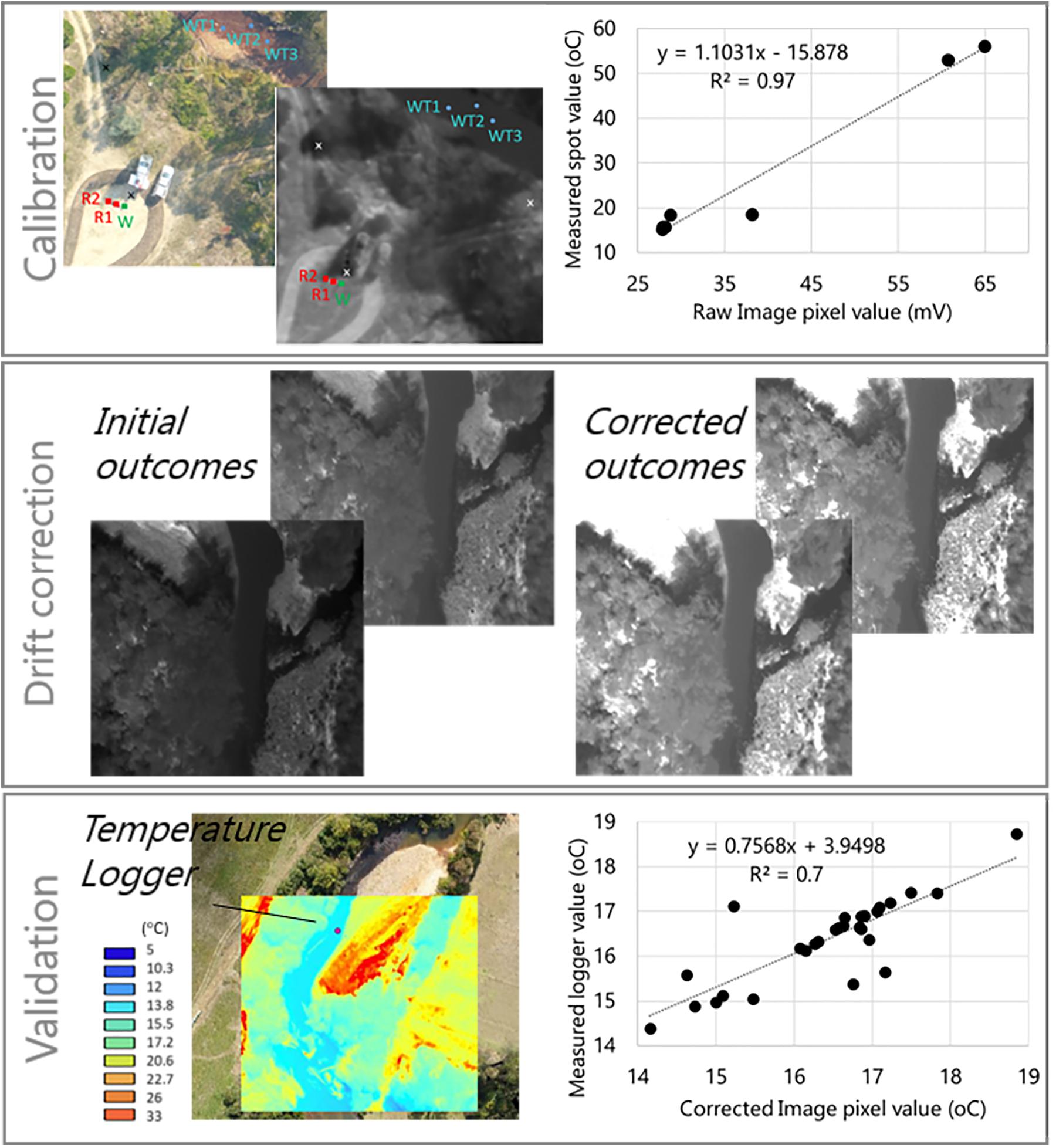
Figure 3. Illustration of the ground thermal calibration targets used in one of the flights as an input to the linear model for TIR imagery thermal calibration (top), outputs of the thermal drift correction (middle), and example of one of the temperature logger location (bottom, left) used as one of the inputs for the final thermal validation (bottom, right).
After each flight, each set of R-JPEG format TIR and RGB images were quickly mosaicked in situ and quality-checked using the Pix4D® (Pix4D, Lausanne, Switzerland) software (Figure 2). For low-quality results, the flights were repeated. Final imagery data was safely stored and organized by type (RGB or TIR), downstream order, day and flight number.
Processing
For the initial thermal calibration, we used the ResearchIR Max® software to convert brightness readings (in mV) from the raw images (R-JPEG format) to temperatures. We took the first image from the base of each TIR flight (Figure 2) and compared it to the ground-truth data (hot, cold, and river ground calibration targets, Figure 3) to fit a linear model to the brightness vs. temperature (all resulting R2-values were between 0.9 and 1, Figure 3). Assuming no change in temperatures during the duration of the flight, the linear model was applied to the subsequent images of the flight in Matlab®. In practice, however, thermal correction of the calibrated images was required where image-level temperature drifting was detected. Image-level temperature drifting is frequently observed for uncooled TIR detectors due to the variable conversion parameters from the raw power values to the temperature output (Ribeiro-Gomes et al., 2017; Dugdale et al., 2019). We corrected image-to-image temperature bias using a Partially Overlapped Histogram Equalization or POHE (Drusch et al., 2005; Su and Ryu, 2015) adapted to TIR imagery processing. POHE removed image-to-image bias from a reference image by equalizing histograms over their overlapping part. We corrected individual images against the reference images that contained the ground thermal targets by matching histograms of the pixel-level brightness in the image overlaps. The thermal reference image was usually the first or the last photo taken at each flight, and we used it to correct all successive images within. Despite showing some loss in pixel resolution, the correction successfully removed the image-level thermal drifting without changing the temperature variation (Figure 3).
Following image-level correction, we used the Pix4D® software to orthomosaick individual images of each flight into 49 of each optical (RGB) and TIR raster tiles. Initial orthomosaicking was based on the imagery onboard GPS data. We used more accurate DGPS locations of the GCPs for georectification to ensure correct overlapping between RGB and TIR raster imagery (Figure 2).
Although the timeseries of stream temperature measured by loggers indicated very low temperature changes within the flight time windows, the potential temporal temperature variation was adjusted to enable the spatial assessment of stream temperature patterns along the river length. The stream temperature logger data on 5 April 2017 at 12:10 h (middle of the survey) was used as the reference to convert TIR imagery collected over the duration of the survey to a temporal-variation-removed image that is equivalent to a snapshot at the reference time. We assumed that the distribution and size of CWPs between the start and the end of the survey time windows remained invariant. We applied a simple linear adjustment to each entire raster based on the data available from the loggers and the pixel values of their location. Thirty-one logger data points (Figure 3) could be used and were visible for approximately 40 TIR raster images (between 1 and 3 loggers per raster, with several loggers visible over two rasters). For those raster imagery with no visible logger data, we used the corrected overlapping imagery from the previous flight to correct the raster. The linear adjustment was done using ArcGIS® 10.4 (Esri) software.
For thermal validation, we used the corrected thermal imagery data prior to adjustment. Temperature values recorded from loggers at the time of imagery acquisition with the corrected pixel values (average 4–6 pixels) of their location within each TIR tiles. The comparison between logger value and corrected pixel data resulted in R2 = 0.7 (Figure 3).
Data Interpretation
Visibility of the Upper Ovens river was possible for the totality of the waterbody in most reaches, given the openness of the channel. Only along the lower reaches, where more constrained channels were partially covered by overhanging vegetation, visibility was still possible for more than three-quarters of the water body. The high matching overlap between both TIR and optical imagery sets allowed the delimitation of the river edge (or visible water pixels). We used optical imagery to draw the edge, and we then applied such delimitation to the TIR raster, so that the terrestrial area could be cut out and only riverine water temperature visible (Figure 2). Each riverine TIR raster was then polygonized into groups of temperature pixels rounded to the closest whole number to achieve an adequate clustering.
We considered the available range of thresholds to identify CWPs in the literature from 2 to 3°C (Ebersole et al., 2001; U.S. Environmental Protection Agency, 2003; Torgersen and Ebersole, 2012) to 0.5°C (Dugdale et al., 2013; Monk et al., 2013; Wawrzyniak et al., 2016; Fullerton et al., 2018) difference with the main channel temperature. After some preliminary testing on data coherence, we selected the polygons presenting variations in temperature higher than 1°C between the minimum temperatures in the CWPs and the mean stream temperature, and we only included polygons >1 m2. We visually checked the optical imagery for each of the identified CWPs and removed artifacts or non-true water patches (e.g., shade on the edge of the gravel).
We obtained the minimum temperature for each CWPs by overlapping the identified polygons to their corresponding corrected TIR raster tile and extracting pixel values statistics (CWPs thermal characterization). We calculated mean stream water temperature by extracting pixel point values at 50 m intervals along the river thalweg from the corrected TIR raster tile. We then averaged the extracted temperature values (between 12 and 20 data points) for each tile.
CWPs were classified into five types based on several existing classifications (Ebersole et al., 2003a; Torgersen and Ebersole, 2012; Dugdale et al., 2013; Kurylyk et al., 2014). They included deep pools, tributaries, cold side channels, emergent hyporheic water, and shading (Figure 4). Tributary plumes are generated by cold tributaries joining the (warmer) main river channel. Cold side channels are lateral channels that usually emerge from seasonally scoured flood channels. Emergent hyporheic water results from the resurgence of hyporheic flow from the streambed, and it is generally detected at the downstream ends of gravel bars, mid-channel islands, or in sequence with pool-riffle bedforms (Wawrzyniak et al., 2016). Although deep pools are usually formed as a result of stratification, their presence in the Upper Ovens were most likely linked to hyporheic water emerging in pool-riffle sequences, but we did not differentiate between the two. In the case of shading, we considered shading was the sole driver of CWP when the CWP delimitation had the same shape and extent of the visible shading in the RGB image. In addition, we considered shade as a potentially added effect promoting other types of CWPs when shade was observed but differed from the extent and shape of the CWP.
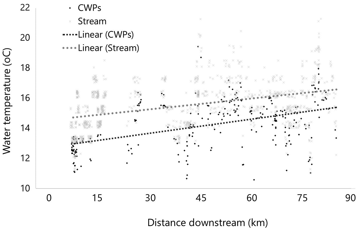
Figure 4. Longitudinal changes in mean stream water temperatures and minimum CWPs temperatures. Note the clusters of no data in the graph reflect the urban areas of Bright and Porepunkah, where no data could be collected, due to flight safety restrictions.
The classification of CWPs helped interpret the potential origin of the cooler water and allowed comparisons to similar studies. We used QGIS (QGIS Development Team, 2019) to enable the visualization of the selected CWP over the optical imagery, so we classified CWPs based on their definition and characterized all key physical attributes associated with each CWP. The exercise was carried out by the same person throughout the whole dataset to minimize its subjectivity.
Associations of CWPs With Physical Controls at Multiple Spatial Scales
A total of 17 physical controls potentially influencing the distribution of CWPs in the Upper Ovens at multiple spatial scales were investigated, including a suite of geomorphological variables and metrics, channel characteristics, riparian vegetation types, land use, and geology (Table 1).
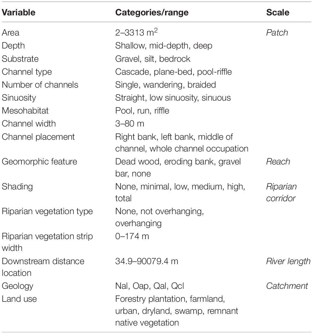
Table 1. Multi-spatial physical controls of cold-water patches considered.
At the patch scale (within each CWP), physical controls were characterized using optical (RGB) imagery data. They included the area occupied by each CWP (polygon area in m2); dominant substrate type within the CWPs (gravel, silt, bedrock) and CWPs depth (shallow, mid-depth, deep), both visible thanks to low flows and clear water conditions. At the reach scale (∼50–500 m), surrounding each CWP, the following qualitative and quantitative information was extracted from optical imagery: channel type (cascade, plane-bed, and pool-riffle, Montgomery and Buffington, 1998); number of channels (single, wandering, braided); sinuosity (straight, low, sinuous); mesohabitat type (pool, run, riffle); channel width (in m); and the CWPs placement and occupation in the channel (right bank, left bank, middle of channel, whole channel occupation). In addition, any key geomorphic feature located within or nearby each CWPs (gravel bar, eroding bank, dead wood, none) were recorded. Physical controls at the riparian corridor scale (along the river) were characterized based on the information provided by optical imagery. The riparian vegetation strip width (ranging from 0 to 174 m) was measured; and the riparian vegetation type was classified for each bank into combinations of none, not overhanging and overhanging vegetation, represented by numerical levels from 1 to 6 (e.g., none in either banks = 1, overhanging vegetation in both banks = 6). In addition, we considered important to characterize the degree of shading present at each CWP at the time of the flight to account for a potential combination of cooling effects. Shading was characterized into six categories including total for 81–100% of CWP area occupied by shade, high for 61–80% shade occupation, medium for 41–60%, low for 21–40%, minimal for 11–20%, and none, for 0–10%. At the river-length scale, the downstream distance location of each CWP was calculated by computing the cumulative linear distance between successive CWPs. At the catchment scale (∼50–100 km), both geology and the surrounding land use were considered catchment controls. Geology information was extracted from the GIS layers provided by the Victorian State Government. It included four main groups: Quaternary non-marine colluvial (Qc1) and alluvial (Qa1) sedimentary rocks, Ordovician marine sedimentary rock (Oap), and Neogene non-marine alluvial sedimentary rock (Na2). Land use was characterized for each of the banks based on optical imagery. To simplify the long list of classes from the original classification, we grouped them into two main groups: anthropogenic (forestry plantation, farmland, urban, industrial) and natural (dryland, swamp, remnant native vegetation). When one of each group was present at each of the banks surrounding the CWPs, a third group (mixed) was assigned (Table 1).
To assess the relationship between the above mentioned physical controls and CWPs, we used a general linear model approach (with normal -Gaussian- errors) using the function glm() in R (R Core Team, 2019). To enable relative comparisons, we used the difference between the mean stream temperature and the minimum temperature of each selected CWP as the response variable. Histograms of the temperature difference suggested a weak right skew, so the response variable was square-root transformed.
The 17 predictor factors (Table 1) consisted of 5 continuous and 12 categorical variables. Of the categorical variables, we treated those with no ordered relationship as factors in the analysis. Categorical variables with a clearly ordered relationship (e.g., high, medium, low) were coded in the analysis as numeric variables representing their ranked order. Scatterplots of temperature difference against the ordered categories showed that any associations were monotonic (i.e., decreasing, increasing level), so we considered a regression on the ranked order to represent the underlying association. We examined continuous variables for normality and collinearity. Distance downstream was weakly positively skewed and was centralized by a square root transformation. Area was also positively skewed, and a log transformation centralized its distribution. A combination of variance inflation factors (VIF) and bivariate scatterplots was used to assess collinearity between numeric variables. With all VIFs < 5, no evidence of collinearity was found. Linear dependence in the categorical regressors was evaluated by examining the model parameterization via the alias() function in R, which found no evidence of dependence between categorical factors and levels.
We calculated an initial linear model of temperature difference against all the hypothesized predictor variables. Initial diagnostics showed that a standard linear model with normal errors was appropriate. Many predictors did not contribute to the analysis, so we reduced the model using a full-stepwise regression with the MASS:stepAIC() function in R. The stepAIC() function uses Akaike’s Information Criterion to compare competing models and penalizes models for numbers of variables retained. Automated stepwise approaches are not guaranteed to find the most appropriate model, so we examined the entry and exits of variables in the model and explored alternative models in a structured approach. Extensive examination of alternatives showed that stepwise selection retained a consistent set of reliable predictors. Analytical assumptions of the final model were assessed graphically by plots of residuals vs. expected values, and normality residuals. We found no critical deviations from analytical assumptions. The effects of the variables in the model were assessed for significance with a threshold of 0.05.
Results
Spatial Patterns of CWPs
A total of 264 CWPs were identified along the 50 km stretch (ca. 95 km in total river length) of the Upper River. CWPs showed highly variable minimum temperatures ranging from 10.5 to 19.4°C along the river length, with relatively lower temperatures compared to mean stream temperature (12.5–19.6°C). Despite high local variability, both CWPs and mean stream temperature showed an increasing trend with downstream distance estimated in 0.14 and 0.17°C per linear kilometer (Figure 4).
Classification based on optical imagery was possible for 260 of the CWPs. Of those, 130 were classified as emergent hyporheic waters, 74 as deep pools, 41 as shading, 11 as side channels, and 4 as tributaries (Figure 5). CWPs promoted thermal differences that ranged between 0.15 and 5°C (based on the pixel data extracted post CWP identification) when compared to the mean stream temperature. Mean thermal differences changed notably depending on the CWPs type, with tributary being the highest and emergent hyporheic water the lowest (Figure 6).
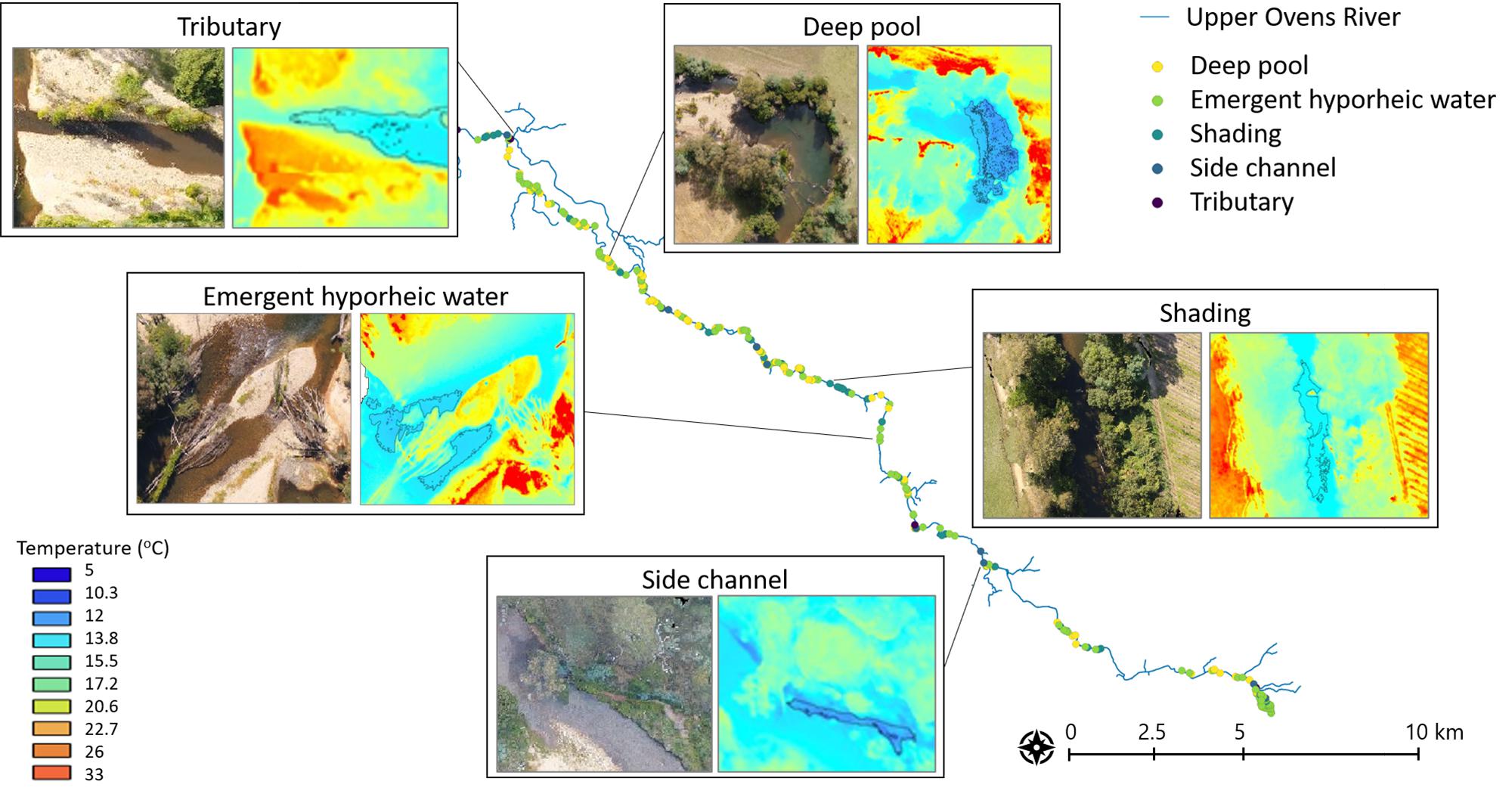
Figure 5. Illustrations of examples for each of the four CWPs types identified, and their locations, along the Upper Ovens River.
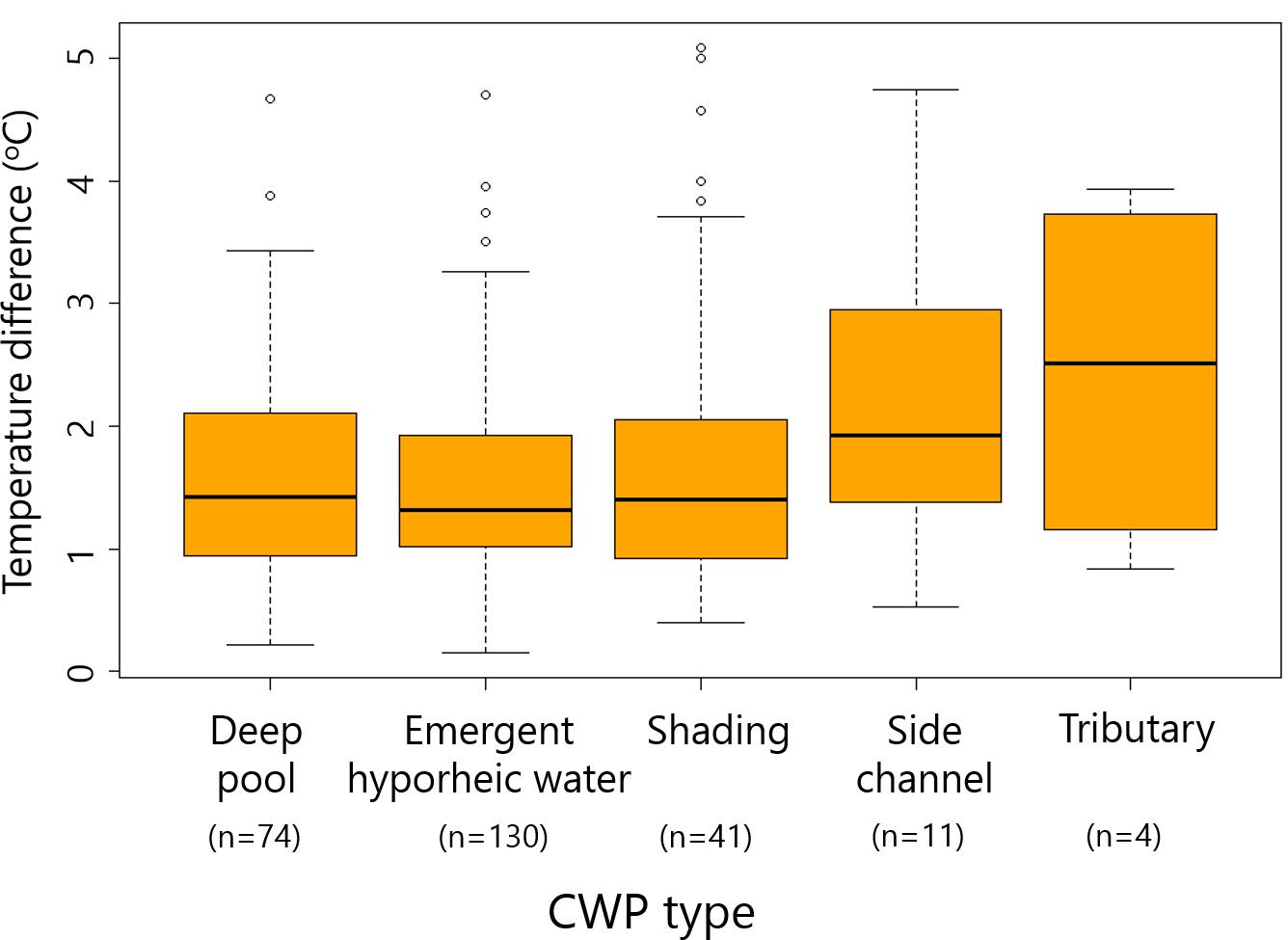
Figure 6. Range of temperature differences promoted by each CWP type in relation to the main channel average temperature. Note that n refers to the number of data points for each CWP type.
CWPs were non-uniformly distributed along the ca 95 km Upper Ovens River length (Figure 7). As with CWPs numbers, the total area occupation by CWPs was higher for emergent hyporheic water types (48,377 m2), followed by deep pools (27,671 m2), shading (16,961 m2), side channels (4,325 m2), and tributaries (632 m2). Individual CWPs presented a broad range or area size, but shading types showed the highest average (4,134 m2), closely followed by side channels (3,934 m2), deep pools (374 m2) and emergent hyporheic water (3,724 m2); and tributary types being again the lowest (158 m2). In terms of relative abundance, the number of emergent hyporheic water CWPs decreased, while deep pools, shading, and tributaries showed an increase with downstream distance (Figure 7).
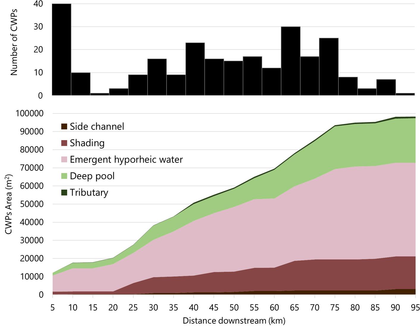
Figure 7. Distribution of CWP numbers (top) and cumulative distribution of CWP types by occupied area (bottom) along the Upper Ovens River.
Most side channels, emergent hyporheic water, and tributaries were associated with gravel bars (91, 77, and 67%, respectively). To a lower degree, deep pools were also associated with gravel bars (42%), and with dead wood (27% of occasions). In contrast, shading was not associated with any geomorphic feature in most cases (63%).
Key Physical Controls Influencing Thermal Differences Promoted by CWPs
An initial variable assessment excluded channel type from the model analysis as it did not show any significant association, possibly because pool-riffle type dominated in all except a few samples. The remaining variables were progressively excluded to achieve the best performing model.
The relative thermal difference promoted by CWPs changed with their channel location, riparian vegetation level or type, area, distance from the source, and land use (Table 2). The standardized regression coefficients enable comparison of relative strengths of each numeric factor. The area of the CWP had the most considerable effect of the continuous variables, with the relative thermal difference promoted by CWP increasing with their area. The magnitude of this difference was in the order of 2°C from the smallest (bottom five, 2–3 m2) to the largest (top five, 2,700–3,317 m2) patches (Figure 8A). Temperature differences were greater in higher levels of riparian vegetation (e.g., with overhanging vegetation in both banks). Average temperature differences from the least to the most vegetated were in the order of 1°C. However, the spread of values and extremes of the differences ranged up to 5°C in areas with dominating overhanging vegetation (Figure 8B). In contrast, relative temperature differences – after taking other factors into account – were lower than expected with increased distance away from the source (Figure 8C). This effect was relatively weak, however.
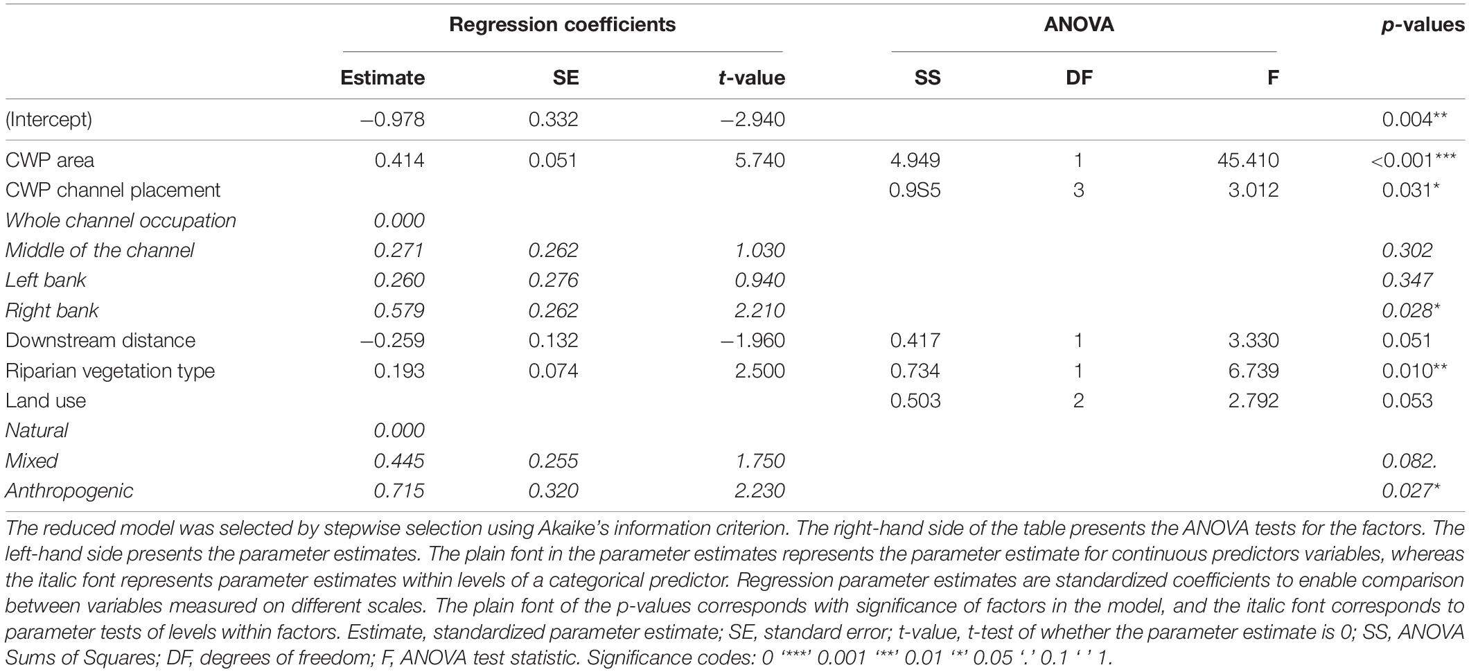
Table 2. Outputs of the general linear model of the relationship between thermal differences promoted by CWPs (square-root transformed) and hypothesized predictions.
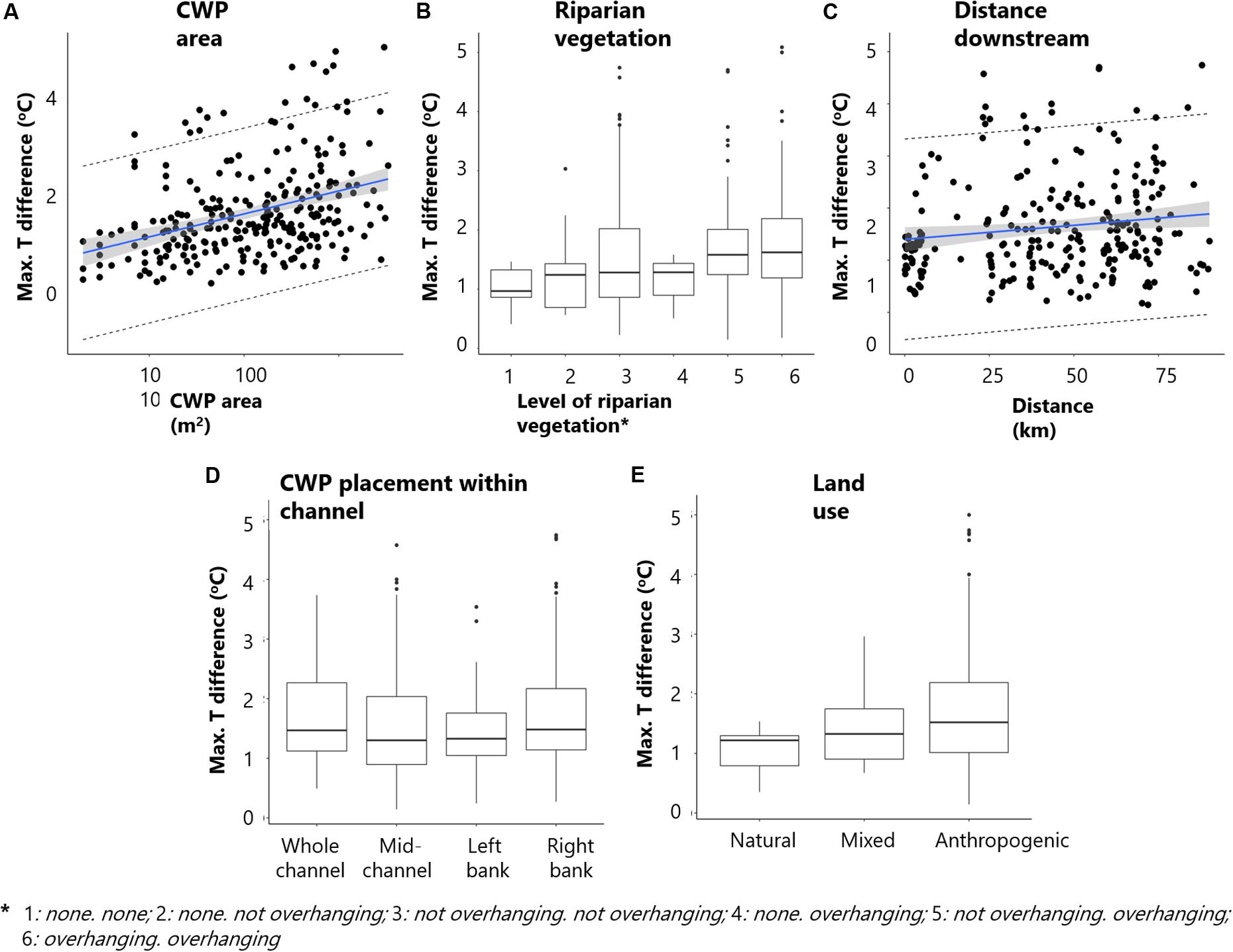
Figure 8. Key variables influencing the maximum thermal difference promoted by CWPs, according to the final selected model. They include CWP area (A), Riparian vegetation (B), distance downstream (C), CWP placement within channel (D), and land use (E).
Channel placement had a weak but significant effect on temperature difference promoted by CWPs (Table 2). Differences in temperature promoted by CWPs that occupied the whole channel were similar to those CWPs located in the right bank. Both were higher than those that were in the middle of the channel and left bank, respectively (Figure 8D). Model outputs suggest that land use had a marginal effect on the overall analysis, with a p-value just above the minimum 0.05 significance threshold. However, an apparent effect was evident between land use levels (Figure 8E). Temperature differences promoted by CWPs increased with the degree of anthropogenic changes to the landscape, with a maximum range of 5°C in the most modified areas. The range of such thermal differences was narrower or more similar within Natural land use types. In contrast, the thermal range was broader, or more variable, within Anthropogenic land use types (Figure 8E).
Discussion
Challenges and Opportunities of the Methodological Approach
We used simultaneous UAV flights to acquire and generate 95 km river length of georeferenced high-resolution TIR and optical orthomosaicked imagery sets, distributed into 49 raster tiles. With these data, it was possible to identify riverscape spatial patterns of temperature and CWPs, and to detect, characterize, classify, and compare discrete CWPs.
The survey in the Ovens river was carried out during the lowest flow period with water still running through, allowing for full hydraulic mixing. In addition, spot temperature measurements in selected accessible deep pools showed almost identical temperatures across the water column (see more details in Casas-Mulet, 2018). Based on these, we assumed no thermal stratification and considered that the caption of surface water temperatures could be used as a representative measurement across the whole water depth. Given the high groundwater dominance in the system, we acknowledge, however, that other methods may be most appropriate for the purposes of direct measurements of groundwater inflow locally (e.g., Gaona et al., 2019). The assessment of river-length scale longitudinal stream temperature patterns can only be realized using absolute values (Loheide and Gorelick, 2006; Wawrzyniak et al., 2013). In this study, this was possible based on the assumption that minimal changes in thermal heterogeneity composition occurred between and within the daily time window of TIR data acquisition. We considered it a reasonable assumption since we carried out all UAV flights during constant low flows on five consecutive days of near-identical climatic conditions, using the same equipment throughout the survey. Minimal changes in stream temperature during the surveying period, confirmed by continuous logging temperature data, also support the assumption. However, to enable comparable interpretations of the outcomes without having to rely on assumptions, the identification of CWPs was based on relative thermal values, taking mean stream temperature as a reference.
Low flows in the Upper Ovens promoted high thermal contrasts between surface and groundwater that enabled the detection of CWPs. The use of adequate cameras and relatively low altitude (sufficient to visualize land features to allow orthomosaicking) drone flights produced high-resolution on-ground pixel size imagery. The ground sample (pixel) distance, or GSD, was approximately 0.1 m for TIR, and 0.05 m for optical (RGB) imagery. Such resolutions greatly aided the detection and identification of CWPs. Low-velocity flights ensured clear color contrast within images and allowed high imagery overlap, both reducing the risks of failure in photogrammetric orthomosaicking reported in Ribeiro-Gomes et al. (2017). High-quality imagery also supported the physical characterization and classification of CWPs. It provided a clear visualization of the river bottom to qualitatively differentiate physical characteristics such as depth and substrate, to identify key geomorphic features such as dead wood and fallen trees, and to assess the degree of shade within all CWPs types.
The delineation of water pixels can be achieved using TIR when water temperature values are within a different range from the surrounding land. Since this was not the case in this study, we took the co-registered TIR and RGB images and used RGB imagery to delineate the river boundaries manually. Given the high matching overlap between both imagery sets, this approach was considered suitable to help identify CWPs polygons. However, the inclusion of co-registered multispectral (VISNIR)-TIR imagery (e.g., Turner et al., 2014) should be considered in future studies to accurately delineate true-water pixels through automatic detection.
The linear models used for TIR calibration were based on in situ ground data (hot, cold, and river water thermal references) taken simultaneously during the flights and implemented consistently throughout the dataset. The linear models provided satisfactory outcomes with high R-square values and accurate TIR imagery. High R-square numbers from a small number of data points needs to be interpreted with caution, however, this is a common limitation in remote sensing, particularly when data collection needs to be completed within a very short time window. Our calibration approach can be compared to the reportedly improved accuracy calibration based on in situ data in Wawrzyniak et al. (2013), only that the use of different media/material for cold (water) vs. hot (rubber) targets, whose temperature were measured using various measurement equipment, might have caused errors originating from varying emissivity between the targets and different nature of radiometric and thermo-couple-based sensors. Ideally, multiple calibration targets that have emissivity values close to the primary survey target (e.g., water in this case) should be used, despite the potential logistical inconveniences.
Almost all calibrated TIR imagery presented some thermal drift that required further correction, a common issue for uncooled bolometer, and reported in Dugdale et al. (2019) and Ribeiro-Gomes et al. (2017). The partially overlapped histogram equalization (POHE) approach used in this study provides a trade-off solution between removing thermal drifting with resulting unchanged actual temperature values and the loss of pixel resolution. The loss of pixel resolution may produce issues in detecting GCPs when orthomosaicking in the photogrammetric process (Ribeiro-Gomes et al., 2017), however, in this study, this was not an issue, as a result of the high-resolution imagery acquired originally. Besides, TIR validation using temperature logger data suggest satisfactory results, albeit the difficulty of processing such an extensive dataset.
Despite the limitations of currently available UAV-based imagery acquisition devices described in Dugdale et al. (2019), this study demonstrated that with the adequate data acquisition, processing, and interpretation approaches, a reliable assessment of river-length patterns of CWPs could be achieved. Overall, the methodological approach described in this study enabled the exploration of CWPs distribution and supported the development of a preliminary model to investigate patterns of potential thermal refuges at multiple spatial scales, contributing to a better understanding of stream thermal heterogeneity drivers (Webb et al., 2008; Monk et al., 2013). This study also provides an opportunity to explore the potential of integrated UAV-TIR systems to assess CWPs patterns across rivescapes.
Spatial Patterns and Controls of CWPs
The non-homogeneous distribution of CWPs aligns with the study of Wawrzyniak et al. (2016) in the Ain River, of comparable dimensions and total CWPs area occupation. The dominance of emergent hyporheic water CWPs seems consistent with the expected groundwater inputs in a gaining system as the Upper Ovens (Yu et al., 2013). Higher thermal differences in tributary CWPs suggest that air-water or altitude-controlled processes may provide cooler waters, either due to the higher shading in such narrower streams (Monk et al., 2013) or their steepness (Webb et al., 2008; Dugdale et al., 2015).
The outputs of the general linear model illustrate a combination of five key physical controls associated with thermal differences in CWPs at multiple spatial scales. They include catchment-scale land use, type of riparian vegetation along the river corridor, downstream distance, reach-scale CWP channel placement, and patch-scale CWP area. While we acknowledge that the model assigns similar larger scale physical controls to different CWPs (e.g., same catchment control > 1 km2, over several CWPs < 1 m2), this approach is based on a thorough assessment of the importance of the control variables and their influences at different spatial scales. Surprisingly, the presence of geomorphic features at the reach scale did not appear to be a key driving factor of CWPs in our modeling, despite evidence of individual associations between gravel bars and emergent hyporheic water CWPs types, as per in Wawrzyniak et al. (2016). However, our modeling approach did not target specific CWPs types; it instead aimed at providing an overall view of driving factors; therefore, the data resolution could have played a role in the analysis.
According to the model outcomes, Anthropogenic land use types seem to promote cooler CWPs. However, in the Upper Ovens, the effects of land use cannot be interpreted without considering its links to both the riparian corridor (LeBlanc et al., 1997; Allan, 2004) and distance downstream. The upper reaches were dominated by natural open riparian forests surrounding multiple-channel braided and wandering reaches with limited shading. In contrast, the lower reaches were surrounded by anthropogenic land use (e.g., arable land) and presented more constrained channels with narrow, but heavily overhanging shading riparian vegetation. Such a local shading effect in the downstream reaches could potentially have increased thermal differences between the river and any type of CWPs, as opposed to the upstream reaches. At the reach scale, the slightly greater cooling effect on the right vs. left bank could reflect the river east-west flow direction, with less sun exposure and increased shading on the right (north-looking). Based on these, it is counterintuitive that the model did not consider shading as an important physical control. We can only assume that the complex physical structure in the Upper Ovens River, combined with the surveying timings and locations played a role, resulting in shading not being strong enough to dent all the other factors, and therefore not represented in the model outcome. At the patch-scale, thermal differences promoted by CWPs increase with the CWPs area. The spatial variation in groundwater influx can likely explain the lack of homogeneous longitudinal patterns in CWPs areas. Patch-scale CWPs area could be interpreted as the local manifestations of larger-scale patterns. Groundwater influxes were variable along the Upper Ovens length, with peaks in the upper and middle reaches (Bright and Porepunkah), as indicated in Casas-Mulet (2018) and Yu et al. (2013). Historical anthropogenic activities could have further influenced such variations (e.g., river dredging, Sinclair Knight Merz, 2007; Yu et al., 2013) by modifying the groundwater inputs mechanisms. For example fine sediment accumulation in the riverbed gravels over time (Casas-Mulet et al., 2017; Auerswald and Geist, 2018; Wilkes et al., 2019) could have clogged the gravels and decrease the amount of emergent hyporheic flow (Poole et al., 2006; Arrigoni et al., 2008). Consequently, the methodological approach described here may also be useful when it comes to assess the effects of river management actions on the distribution and persistence of CWPs, such as streambed restoration actions or groundwater extraction restrictions.
The outcomes of this study illustrate the influence of several multi-spatial scale physical controls on CWPs that had not been assessed in conjunction before. Future works should focus on integrating ecological processes into spatio-temporal riverscape patterns, so the true thermal refugia potential of CWPs is understood.
Applications in Freshwater Conservation and Management
In Australia, an increased recurrence of drought conditions will intensify cease-to-flow events and potentially lower ground-water levels (CSIRO and Bureau of Meteorology (BOM), 2007; IPCC, 2012). Although extreme events are crucial elements of the natural variability shaping the ecology of rivers that enable freshwater organisms recovering from disturbances, intensified pressures could hinder the capacity of communities to persist (Leigh et al., 2015). In addition, anthropogenic threats such as the increasing demands of water retention, diversion and extraction for agricultural irrigation (Pratchett et al., 2011; van Dijk et al., 2013) put increasing pressure on freshwater habitats, lessening the potential resilience of aquatic organisms (Kohen, 2011; Leigh et al., 2015).
Associated effects of increased stream temperature include reduced dissolved oxygen and can result in the physiological tolerance of some species being exceeded (e.g., McNeil and Closs, 2007). Increased stream temperatures may also affect development, growth rates, reproduction, and behavior of organisms. These could favor species with wider thermal windows (Pörtner and Farrell, 2008), or promote the establishment of and spread alien species of fish when coupled with other stressors such as the reduction in discharge (Morrongiello et al., 2011). The availability of CWPs may buffer the effects of extreme events and prevent pushing some ecological processes beyond critical thresholds, protecting species persistence, and maintaining ecosystem functioning (Leigh et al., 2015).
The identification of CWPs is, therefore, the first step toward their conservation and sustainable management (Kurylyk et al., 2014; Geist, 2015). Predictions of CWPs locations and distribution can help prioritize river restoration measures such as targeted riparian vegetation planting to increase shading (Ebersole et al., 2015; Morelli et al., 2016; Fullerton et al., 2018), or in-stream habitat restoration (Gilvear et al., 2013; Pander et al., 2018) with a focus on promoting hyporheic upwelling (Boulton et al., 2010; Pander et al., 2015). Identification and prioritization of the most effective ways of conserving or restoring CWPs also greatly benefit from an evidence-based management approach (Geist and Hawkins, 2016) that requires comparison with baseline data. The identification of water quality thresholds will be required to inform water-allocation decision making (Goulburn Murray Water, 2011) and to manage and protect surface and subsurface induced CWPs. Identifying the factors that give alien species competitive advantages or disadvantages over native species will be key requirements for managing CWPs under climate change. In particular, it will be essential to consider that some aliens will benefit from warmer temperatures, whereas others will be detrimentally affected (e.g., Costelloe et al., 2010).
Further work is needed, building on this and other exploratory studies, to develop tools to predict the distribution of potential thermal refugia at the riverscape, which will be critical to inform long-term measures that maintain resilient thermal landscapes (Bond et al., 2008; Monk et al., 2013; Fullerton et al., 2018). A better understanding of the spatio-temporal extent over which promoting stream thermal refugia can be an effective adaptation tool is required (Morrongiello et al., 2011), and it will enable its integration into legislation and policy frameworks.
Data Availability Statement
The datasets generated for this study are available on request to the corresponding author.
Author Contributions
RC-M designed the study, planned and supervised the fieldwork, and carried out the data processing and analysis in consultation with DR. RC-M, JG, and JP conceived the idea of the manuscript and wrote the manuscript in consultation with DR and MS. All authors read and approved the final version of the manuscript.
Funding
The funding for the data acquisition and post-processing of this study came from the North East Catchment Management Authority (NECMA, Victoria, Australia). Data acquisition was also supported by MS’s ARC Discovery Project DP130103619. The writing part of the work by RC-M was done as part of her Alexander von Humboldt Fellowship at TUM.
Conflict of Interest
The authors declare that the research was conducted in the absence of any commercial or financial relationships that could be construed as a potential conflict of interest.
Acknowledgments
The authors would like to thank Catherine McInerney at NECMA for the logistic support throughout the data collection, and the Murray-Darling Freshwater Research Centre for data provision. UAV-based data acquisition was carried out by XM3 Aerial. We are grateful to the whole team of professionals, and several helpers for the enthusiasm and flexibility shown during the enduring field campaign. Special thanks to Anne Yue Wang and Kate Suyoung Park to help organise and quality-check imagery data prior, during, and after the field campaign. Many special thanks as well to Lance Larr for the valuable help developing the partial overlapping histogram equalisation Matlab-based tool suited to the dataset. Finally, we thank Aimee H. Fullerton and Jens Kiesel for their thorough and constructive review of the manuscript.
References
Allan, J. D. (2004). Landscapes and riverscapes: the influence of land use on stream ecosystems. Annu. Rev. Ecol. Evol. Syst. 35, 257–284. doi: 10.1146/annurev.ecolsys.35.120202.110122
Arrigoni, A. S., Poole, G. C., Mertes, L. A. K., O’Daniel, S. J., Woessner, W. W., and Thomas, S. A. (2008). Buffered, lagged, or cooled? Disentangling hyporheic influences on temperature cycles in stream channels. Water Resour. Res. 44, 1–13. doi: 10.1029/2007WR006480
Auerswald, K., and Geist, J. (2018). Extent and causes of siltation in a headwater stream bed: catchment soil erosion is less important than internal stream processes. Land Degrad. Dev. 29, 737–748. doi: 10.1002/ldr.2779
Australian Government Bureau of Meteorology, (2018). Water Discharge Data [WWW Document]. Available at: http://www.bom.gov.au/waterdata/ (accessed March 22, 2018).
Bond, N. (2007). Identifying, Mapping and Managing Drought Refuges : A Brief Summary of Issues and Approaches eWater Cooperative Research Centre Technical Report. Canberra: eWater Cooperative Research Centre.
Bond, N. R., Lake, P. S., and Arthington, A. H. (2008). The impacts of drought on freshwater ecosystems: an Australian perspective. Hydrobiologia 600, 3–16. doi: 10.1007/s10750-008-9326-z
Boulton, A. J. (2003). Parallels and contrasts in the effects of drought on stream macroinvertebrate assemblages. Freshw. Biol. 48, 1173–1185.
Boulton, A. J., Datry, T., Kasahara, T., Mutz, M., and Stanford, J. A. (2010). Ecology and management of the hyporheic zone: stream-groundwater interactions of running waters and their floodplains. J. North Am. Benthol. Soc. 29, 26–40. doi: 10.1899/08-017.1
Braun, A., Auerswald, K., and Geist, J. (2012). Drivers and spatio-temporal extent of hyporheic patch variation: implications for sampling. PLoS One 7:e42046. doi: 10.1371/journal.pone.0042046
Caissie, D. (2006). The thermal regime of rivers: a review. Freshw. Biol. 51, 1389–1406. doi: 10.1111/j.1365-2427.2006.01597.x
Carbonneau, P., Fonstad, M. A., Marcus, W. A., and Dugdale, S. J. (2012). Making riverscapes real. Geomorphology 137, 74–86. doi: 10.1016/j.geomorph.2010.09.030
Casas-Mulet, R. (2018). Assessment of Potential Drought Refuges in the Upper Ovens River Based on UAV Thermal InfraRred Imagery (TIR). Melbourne: MUASIP.
Casas-Mulet, R., Alfredsen, K. T., McCluskey, A. H., and Stewardson, M. J. (2017). Key hydraulic drivers and patterns of fine sediment accumulation in gravel streambeds: a conceptual framework illustrated with a case study from the Kiewa River, Australia. Geomorphology 299, 152–164. doi: 10.1016/j.geomorph.2017.08.032
Corti Meneses, N., Baier, S., Reidelstürz, P., Geist, J., and Schneider, T. (2018a). Modelling heights of sparse aquatic reed (Phragmites australis) using Structure from Motion point clouds derived from Rotary- and Fixed-Wing Unmanned Aerial Vehicle (UAV) data. Limnologica 72, 10–21. doi: 10.1016/j.limno.2018.07.001
Corti Meneses, N., Brunner, F., Baier, S., Geist, J., and Schneider, T. (2018b). Quantification of extent, density, and status of aquatic reed beds using point clouds derived from UAV–RGB imagery. Remote Sens. 10:1869. doi: 10.3390/rs10121869
Costelloe, J. F., Reid, J. R. W., Pritchard, J. C., Puckridge, J. T., Bailey, V. E., and Hudson, P. J. (2010). Are alien fish disadvantaged by extremely variable flow regimes in arid-zone rivers? Mar. Freshw. Res. 61, 857–863. doi: 10.1071/MF09090
Dole-Olivier, M. J., Wawzyniak, V., Creuzé des Châtelliers, M., and Marmonier, P. (2019). Do thermal infrared (TIR) remote sensing and direct hyporheic measurements (DHM) similarly detect river-groundwater exchanges? Study along a 40 km-section of the Ain River (France). Sci. Total Environ. 646, 1097–1110. doi: 10.1016/j.scitotenv.2018.07.294
Drusch, M., Wood, E. F., and Gao, H. (2005). Observation operators for the direct assimilation of TRMM microwave imager retrieved soil moisture. Geophys. Res. Lett. 32, 32–35. doi: 10.1029/2005GL023623
Dugdale, S. J. (2016). A practitioner’s guide to thermal infrared remote sensing of rivers and streams: recent advances, precautions and considerations. Wiley Interdiscip. Rev. Water 3, 251–268. doi: 10.1002/wat2.1135
Dugdale, S. J., Bergeron, N. E., and St-Hilaire, A. (2013). Temporal variability of thermal refuges and water temperature patterns in an Atlantic salmon river. Remote Sens. Environ. 136, 358–373. doi: 10.1016/J.RSE.2013.05.018
Dugdale, S. J., Bergeron, N. E., and St-Hilaire, A. (2015). Spatial distribution of thermal refuges analysed in relation to riverscape hydromorphology using airborne thermal infrared imagery. Remote Sens. Environ. 160, 43–55. doi: 10.1016/J.RSE.2014.12.021
Dugdale, S. J., Kelleher, C. A., Malcolm, I. A., Caldwell, S., and Hannah, D. M. (2019). Assessing the potential of drone-based thermal infrared imagery for quantifying river temperature heterogeneity. Hydrol. Process. 33, 1152–1163. doi: 10.1002/hyp.13395
Ebersole, J. L., Liss, W. J., and Frissell, C. A. (2001). Relationship between stream temperature, thermal refugia and rainbow trout Oncorhynchus mykiss abundance in arid-land streams in the northwestern United States. Ecol. Freshw. Fish 10, 1–10. doi: 10.1034/j.1600-0633.2001.100101.x
Ebersole, J. L., Liss, W. J., and Frissell, C. A. (2003a). Cold water patches in warm streams: physicochemical characteristics and the influence of shading. J. Am. Water Resour. Assoc. 39, 355–368. doi: 10.1111/j.1752-1688.2003.tb04390.x
Ebersole, J. L., Liss, W. J., and Frissell, C. A. (2003b). Thermal heterogeneity, stream channel morphology, and salmonid abundance in northeastern Oregon streams. Can. J. Fish. Aquat. Sci. 60, 1266–1280.
Ebersole, J. L., Wigington, P. J., Leibowitz, S. G., Comeleo, R. L., and Van Sickle, J. (2015). Predicting the occurrence of cold-water patches at intermittent and ephemeral tributary confluences with warm rivers. Freshw. Sci. 34, 111–124. doi: 10.1086/678127
Fausch, K. D., Torgersen, C. E., Baxter, C. V., and Li, H. W. (2002). Landscapes to riverscapes : bridging the gap between research and conservation of stream fishes. Bioscience 52, 483–498.
Frissell, C. A., Liss, W. J., Warren, C. E., and Hurley, M. D. (1986). A hierarchical framework for stream habitat classification: viewing streams in a watershed context. Environ. Manage. 10, 199–214. doi: 10.1007/BF01867358
Fullerton, A. H., Torgersen, C. E., Lawler, J. J., Steel, E. A., Ebersole, J. L., and Lee, S. Y. (2018). Longitudinal thermal heterogeneity in rivers and refugia for coldwater species: effects of scale and climate change. Aquat. Sci. 80, 1–15. doi: 10.1007/s00027-017-0557-9
Gaona, J., Meinikmann, K., and Lewandowski, J. (2019). Identification of groundwater exfiltration, interflow discharge, and hyporheic exchange flows by fibre optic distributed temperature sensing supported by electromagnetic induction geophysics. Hydrol. Process. 33, 1390–1402. doi: 10.1002/hyp.13408
Garner, G., Malcolm, I. A., Sadler, J. P., and Hannah, D. M. (2017). The role of riparian vegetation density, channel orientation and water velocity in determining river temperature dynamics. J. Hydrol. 553, 471–485. doi: 10.1016/j.jhydrol.2017.03.024
Geist, J. (2015). Seven steps towards improving freshwater conservation. Aquat. Conserv. Mar. Freshw. Ecosyst. 25, 447–453. doi: 10.1002/aqc.2576
Geist, J., and Hawkins, S. J. (2016). Habitat recovery and restoration in aquatic ecosystems: current progress and future challenges. Aquat. Conserv. Mar. Freshw. Ecosyst. 26, 942–962. doi: 10.1002/aqc.2702
Gilvear, D. J., Spray, C. J., and Casas-Mulet, R. (2013). River rehabilitation for the delivery of multiple ecosystem services at the river network scale. J. Environ. Manage. 126, 30–43. doi: 10.1016/j.jenvman.2013.03.026
Goulburn Murray Water, (2011). Upper Ovens River Water Supply Protection Area Water Management Plan. Tatura: Goulburn Murray Water.
Handcock, R. N., Torgersen, C. E., Cherkauer, K. A., Gillespie, A. R., Tockner, K., Faux, R. N., et al. (2012). “Thermal Infrared Remote Sensing of Water Temperature in Riverine Landscapes,” in Fluvial Remote Sensing for Science and Management, eds P. E. Carbonneau, and H. Piégay, (Chichester: John Wiley & Sons, Ltd), doi: 10.1002/9781119940791.ch
Hart, B. T., and Doolan, J. (2017). Decision Making in Water Resources Policy and Management: An Australian Perspective, 1st Edn. Amsterdam: Academic Press.
IPCC, (2012). Managing the Risks of Extreme Events and Disasters to Advance Climate Change Adaptation: Special Report of the Intergovernmental Panel on Climate Change, Managing the Risks of Extreme Events and Disasters to Advance Climate Change Adaptation: Special Report of the Intergovernmental Panel on Climate Change. Geneva: IPCC. doi: 10.1017/CBO9781139177245
Isaak, D. J., Young, M. K., Nagel, D. E., Horan, D. L., and Groce, M. C. (2015). The cold-water climate shield: delineating refugia for preserving salmonid fishes through the 21st century. Glob. Chang. Biol. 21, 2540–2553. doi: 10.1111/gcb.12879
James, C., VanDerWal, J., Capon, S., Hodgson, L., Waltham, N., Ward, D., et al. (2013). Identifying Climate Refuges for Freshwater Biodiversity Across Australia, Gold Coast. Gold Coast: National Climate Change Adaptation Research Facility.
Judd, D., Rutherfurd, I. D., Tilleard, J. W., and Keller, R. J. (2007). A case study of the processes displacing flow from the anabranching Ovens River, Victoria, Australia. Earth Surf. Process. Landforms 32, 2120–2132. doi: 10.1002/esp.1516
Kaushal, S. S., Likens, G. E., Jaworski, N. A., Pace, M. L., Sides, A. M., Seekell, D., et al. (2010). Rising stream and river temperatures in the United States. Front. Ecol. Environ. 8, 461–466. doi: 10.1890/090037
Kelly, J., Kljun, N., Olsson, P. O., Mihai, L., Liljeblad, B., Weslien, P., et al. (2019). Challenges and best practices for deriving temperature data from an uncalibrated UAV thermal infrared camera. Remote Sens. 11:567. doi: 10.3390/rs11050567
Keppel, G., Mokany, K., Wardell-Johnson, G. W., Phillips, B. L., Welbergen, J. A., and Reside, A. E. (2015). The capacity of refugia for conservation planning under climate change. Front. Ecol. Environ. 13:106–112. doi: 10.1890/140055
Kohen, J. D. (2011). Climate change and Australian marine and freshwater environments, fishes and fisheries: introduction. Mar. Freshw. Res. 62, 981–983. doi: 10.1071/MF09285
Kurylyk, B. L., Macquarrie, K. T. B., Linnansaari, T., Cunjak, R. A., and Curry, R. A. (2014). Preserving, augmenting and creating cold-water thermal refugia in rivers: Concepts derived from research on the Miramichi River, New Brunswick (Canada). Ecohydrology 8, 1095-1108. doi: 10.1002/eco.1566/abstract
LeBlanc, R. T., Brown, R. D., and FitzGibbon, J. E. (1997). Modeling the effects of land use change on the water temperature in unregulated urban streams. J. Environ. Manage 49, 445–469. doi: 10.1006/jema.1996.0106
Leigh, C., Bush, A., Harrison, E. T., Ho, S. S., Luke, L., Rolls, R. J., et al. (2015). Ecological effects of extreme climatic events on riverine ecosystems: insights from Australia. Freshw. Biol. 60, 2620–2638. doi: 10.1111/fwb.12515
Loheide, S. P., and Gorelick, S. M. (2006). Quantifying stream-aquifer interactions through the analysis of remotely sensed thermographic profiles and in situ temperature histories. Environ. Sci. Technol. 60, 3336–3341. doi: 10.1021/ES0522074
McCluney, K. E., Poff, N. L., Palmer, M. A., Thorp, J. H., Poole, G. C., Williams, B. S., et al. (2014). Riverine macrosystems ecology: sensitivity, resistance, and resilience of whole river basins with human alterations. Front. Ecol. Environ. 12, 48–58. doi: 10.1890/120367
McCullough, D. A., Bartholow, J. M., Jager, H. I., Beschta, R. L., Cheslak, E. F., Deas, M. L., et al. (2009). Research in thermal biology: burning questions for coldwater stream fishes. Rev. Fish. Sci. 17, 90–115. doi: 10.1080/10641260802590152
McNeil, D. G., and Closs, G. P. (2007). Behavioural responses of a south-east Australian floodplain fish community to gradual hypoxia. Freshw. Biol. 52, 412–420. doi: 10.1111/j.1365-2427.2006.01705.x
Miller, L., and Barbee, N. (2003). Environmental Condition of Rivers and Streams in the Ovens Catchment. Seatle, WA: Environmental Protection Agency.
Monk, W. A., Wilbur, N. M., Curry, R. A., Gagnon, R., and Faux, R. N. (2013). Linking landscape variables to cold water refugia in rivers. J. Environ. Manage. 118, 170–176. doi: 10.1016/j.jenvman.2012.12.024
Montgomery, D. R., and Buffington, J. M. (1998). “Channel processes, classification, and response,” in River Ecology and Management, eds R. J. Naiman, and R. E. Bilby, (New York, NY: Springer-Verlag), 13–42.
Morelli, T. L., Daly, C., Dobrowski, S. Z., Dulen, D. M., Ebersole, J. L., Jackson, S. T., et al. (2016). Managing climate change refugia for climate adaptation. PLoS One 11:e0159909. doi: 10.1371/journal.pone.0159909
Morrongiello, J. R., Beatty, S. J., Bennett, J. C., Crook, D. A., Ikedife, D. N. E. N., Kennard, M. J., et al. (2011). Climate change and its implications for Australia’s freshwater fish. Mar. Freshw. Res. 62, 1082–1098. doi: 10.1071/MF10308
Murray-Darling Basin Commission, (2007). River Murray system–Drought Update No. 7 April 2007. Canberra: Murray-Darling Basin Commission.
Ning, N., Stratford, D., Nielsen, D., Baldwin, D., Brown, P., Davis, J., et al. (2015). A Review of Climate Refuge Science and its Applciation in the Murray-Darling Basin. Wodonga, VIC: MDFRC Publication.
Orr, H. G., Simpson, G. L., des Clers, S., Watts, G., Hughes, M., Hannaford, J., et al. (2015). Detecting changing river temperatures in England and Wales. Hydrol. Process. 29, 752–766. doi: 10.1002/hyp.10181
Ouellet, V., Gibson, E. E., Daniels, M. D., and Watson, N. A. (2017). Riparian and geomorphic controls on thermal habitat dynamics of pools in a temperate headwater stream. Ecohydrology 10:e1891. doi: 10.1002/eco.1891
Owuor, S. O., Butterbach-Bahl, K., Guzha, A. C., Rufino, M. C., Pelster, D. E., Díaz-Pinés, E., et al. (2016). Groundwater recharge rates and surface runoff response to land use and land cover changes in semi-arid environments. Ecol. Process. 5:16. doi: 10.1186/s13717-016-0060-6
Palmer, M. A., Reidy Liermann, C. A., Nilsson, C., Flörke, M., Alcamo, J., Lake, P. S., et al. (2008). Climate change and the world’s river basins: anticipating management options. Front. Ecol. Environ. 6, 81–89. doi: 10.1890/060148
Pander, J., Mueller, M., and Geist, J. (2015). A comparison of four stream substratum restoration techniques concerning interstitial conditions and downstream effects. River Res. Appl. 31, 239–255. doi: 10.1002/rra.2732
Pander, J., Mueller, M., and Geist, J. (2018). Habitat diversity and connectivity govern the conservation value of restored aquatic floodplain habitats. Biol. Conserv. 217, 1–10. doi: 10.1016/J.BIOCON.2017.10.024
Poole, G. C., Stanford, J. A., Running, S. W., and Frissell, C. A. (2006). Multiscale geomorphic drivers of groundwater flow paths: subsurface hydrologic dynamics and hyporheic habitat diversity. J. North Am. Benthol. Soc. 25, 288–303.
Pörtner, H. O., and Farrell, A. P. (2008). Ecology: physiology and climate change. Science 322, 690–692. doi: 10.1126/science.1163156
Pratchett, M. S., Bay, L. K., Gehrke, P. C., Koehn, J. D., Osborne, K., Pressey, R. L., et al. (2011). Contribution of climate change to degradation and loss of critical fish habitats in Australian marine and freshwater environments. Mar. Freshw. Res. 62, 1062–1081.
QGIS Development Team, (2019). QGIS Geographic Information System. Open Source Geospatial Foundation Project. Available at: http://qgis.osgeo.org (accessed April 16, 2019)Google Scholar
R Core Team, (2019). R: A Language and Environment for Statistical Computing. Vienna: R Foundation for Statistical Computing.
Reid, A. J., Carlson, A. K., Creed, I. F., Eliason, E. J., Gell, P. A., Johnson, P. T. J., et al. (2019). Emerging threats and persistent conservation challenges for freshwater biodiversity. Biol. Rev. 94, 849–873. doi: 10.1111/brv.12480
Ribeiro-Gomes, K., Hernández-López, D., Ortega, J. F., Ballesteros, R., Poblete, T., and Moreno, M. A. (2017). Uncooled thermal camera calibration and optimization of the photogrammetry process for UAV applications in agriculture. Sensors 17, 9–11. doi: 10.3390/s17102173
Robson, B., Chester, E., Allen, M., Beatty, S., Chambers, J., Close, P., et al. (2013). Novel Methods for Managing Freshwater Refuges Against Climate Change in Southern Australia. Final Report. Gold Coast: National Climate Change Adaptation Research Facility, 59.
Sawyer, A. H., and Cardenas, M. B. (2012). Effect of experimental wood addition on hyporheic exchange and thermal dynamics in a losing meadow stream. Water Resour. Res. 48:W10537. doi: 10.1029/2011WR011776
Sinclair Knight Merz, (2007). Upper Ovens Conceptual Hydrogeological Model. Sydney: Sinclair Knight Merz.
Sinclair Knight Merz, (2013). Upper Ovens River : Ecological Monitoring and Review of FLOWS Reaches and Hydrological Models: Ecological Impacts of Low Flows. Sydney: Sinclair Knight Merz Report VW06797.
Steel, E. A., Beechie, T. J., Torgersen, C. E., and Fullerton, A. H. (2017). Envisioning, Quantifying, and Managing Thermal Regimes on River Networks. Bioscience 67, 506–522. doi: 10.1093/biosci/bix047
Su, C. H., and Ryu, D. (2015). Multi-scale analysis of bias correction of soil moisture. Hydrol. Earth Syst. Sci. 19, 17–31. doi: 10.5194/hess-19-17-2015
Thorp, J. H., Thoms, M. C., and Delong, M. D. (2006). The riverine ecosystem synthesis: biocomplexity in river networks across space and time. River Res. Appl. 22, 123–147. doi: 10.1002/rra.901
Tonolla, D., Acuña, V., Uehlinger, U., Frank, T., and Tockner, K. (2010). Thermal Heterogeneity in River Floodplains. Ecosystems 13, 727–740. doi: 10.1007/s10021-010-9350-5
Torgersen, C. E., Price, D. M., Li, H. W., and Mcintosh, B. A. (1999). Multiscale Thermal Refugia and Stream Habitat Associations of Chinook Salmon in Northeastern Oregon. Ecol. Appl. 9, 301–319.
Torgersen, C., and Ebersole, J. (2012). Primer for identifying cold-water refuges to protect and restore thermal diversity in riverine landscapes. EPA Sci. Guid. Handb. 91:91.
Turner, D., Lucieer, A., Malenovský, Z., King, D. H., and Robinson, S. A. (2014). Spatial co-registration of ultra-high resolution visible, multispectral and thermal images acquired with a micro-UAV over antarctic moss beds. Remote Sens. 6, 4003–4024. doi: 10.3390/rs6054003
U.S. Environmental Protection Agency, (2003). EPA Region 10 Guidance for Pacific Northwest State and Tribal Water Quality Standards. EPA 910-B-03-002. Seatle, WA: Environmental Protection Agency.
van Dijk, A. I. J. M., Beck, H. E., Crosbie, R. S., de Jeu, R. A. M., Liu, Y. Y., Podger, G. M., et al. (2013). The Millennium Drought in southeast Australia (2001–2009): Natural and human causes and implications for water resources, ecosystems, economy, and society. Water Resour. Res. 49, 1040–1057. doi: 10.1002/wrcr.20123
van Vliet, M. T. H., Franssen, W. H. P., Yearsley, J. R., Ludwig, F., Haddeland, I., Lettenmaier, D. P., et al. (2013). Global river discharge and water temperature under climate change. Glob. Environ. Chang. 23, 450–464. doi: 10.1016/j.gloenvcha.2012.11.002
Vörösmarty, C. J., McIntyre, P. B., Gessner, M. O., Dudgeon, D., Prusevich, A., Green, P., et al. (2010). Global threats to human water security and river biodiversity. Nature 467, 555–561. doi: 10.1038/nature09440
Wawrzyniak, V., Piégay, H., Allemand, P., Vaudor, L., and Grandjean, P. (2013). Prediction of water temperature heterogeneity of braided rivers using very high resolution thermal infrared (TIR) images. Int. J. Remote Sens. 34, 4812–4831. doi: 10.1080/01431161.2013.782113
Wawrzyniak, V., Piégay, H., Allemand, P., Vaudor, L., Goma, R., and Grandjean, P. (2016). Effects of geomorphology and groundwater level on the spatio-temporal variability of riverine cold water patches assessed using thermal infrared (TIR) remote sensing. Remote Sens. Environ. 175, 337–348. doi: 10.1016/j.rse.2015.12.050
Webb, B. W., Hannah, D. M., Moore, R. D., Brown, L. E., and Nobilis, F. (2008). Recent advances in stream and river temperature research. Hydrol. Process. 22, 902–918. doi: 10.1002/hyp.6994
Wilby, R. L., Orr, H., Watts, G., Battarbee, R. W., Berry, P. M., Chadd, R., et al. (2010). Evidence needed to manage freshwater ecosystems in a changing climate: Turning adaptation principles into practice. Sci. Total Environ. 408, 4150–4164. doi: 10.1016/j.scitotenv.2010.05.014
Wilkes, M. A., Gittins, J. R., Mathers, K. L., Mason, R., Casas-Mulet, R., Vanzo, D., et al. (2019). Physical and biological controls on fine sediment transport and storage in rivers. Wiley Interdiscip. Rev. Water 6:e1331. doi: 10.1002/wat2.1331
Wohl, E. (2016). Spatial heterogeneity as a component of river geomorphic complexity. Prog. Phys. Geogr. Earth Environ. 40, 598–615. doi: 10.1177/0309133316658615
Yu, M. C. L., Cartwright, I., Braden, J. L., and De Bree, S. T. (2013). Examining the spatial and temporal variation of groundwater inflows to a valley-to-floodplain river using 222Rn, geochemistry and river discharge: the ovens river, southeast Australia. Hydrol. Earth Syst. Sci. 17, 4907–4924. doi: 10.5194/hess-17-4907-2013
Keywords: river resilience, climate adaptation, cold-water spots, thermal refuges, stream temperature, habitat heterogeneity, riparian vegetation, remote sensing
Citation: Casas-Mulet R, Pander J, Ryu D, Stewardson MJ and Geist J (2020) Unmanned Aerial Vehicle (UAV)-Based Thermal Infra-Red (TIR) and Optical Imagery Reveals Multi-Spatial Scale Controls of Cold-Water Areas Over a Groundwater-Dominated Riverscape. Front. Environ. Sci. 8:64. doi: 10.3389/fenvs.2020.00064
Received: 14 February 2020; Accepted: 06 May 2020;
Published: 27 May 2020.
Edited by:
Rafaela Schinegger, University of Natural Resources and Life Sciences Vienna, AustriaReviewed by:
Aimee H. Fullerton, National Oceanic and Atmospheric Administration (NOAA), United StatesJens Kiesel, Leibniz-Institute of Freshwater Ecology and Inland Fisheries (IGB), Germany
Copyright © 2020 Casas-Mulet, Pander, Ryu, Stewardson and Geist. This is an open-access article distributed under the terms of the Creative Commons Attribution License (CC BY). The use, distribution or reproduction in other forums is permitted, provided the original author(s) and the copyright owner(s) are credited and that the original publication in this journal is cited, in accordance with accepted academic practice. No use, distribution or reproduction is permitted which does not comply with these terms.
*Correspondence: Roser Casas-Mulet, roser.casas-mulet@tum.de