One-year spatiotemporal variations of air pollutants in a major chemical-industry park in the Yangtze River Delta, China by 30 miniature air quality monitoring stations

1 Introduction

With the acceleration of urbanization, the number of chemical industrial parks (CIP) in China is growing rapidly at a rate of about 5% every year (An et al., 2021). CIP is characterized with of large area, numerous and densely distributed enterprises, a great amount of dangerous chemicals, complex production processes, etc. (Pascal et al., 2013; Wu et al., 2021). The intermittent and fugitive emissions of air pollutants had caused serious air pollution in CIP and the surroundings, which had caused many complaints from residents (Chen et al., 2019). In recent years, a number of studies on air pollutants in industrial parks mainly focused on the petrochemical industry (Zheng et al., 2020; Jia et al., 2021; Lin et al., 2021), and the iron and steel industry (Wang et al., 2019; Baek et al., 2020; Zhang et al., 2020), etc. Fine chemical industry is one of the most rapidly developing chemical fields today. Fine chemical industry Parks (FCIPs)are non-ignorable sources of air pollutants due to a huge of gaseous pollutants emitted from their production processes. Therefore, it was particularly important to monitor air pollutants in the long-term in FCIP to know the negative effects of air pollutants on surrounding residents and the environment.

At present, the FCIPs generally built one station integrating several monitoring instruments to monitor air quality (Zhang T et al., 2021). It is hard to build enough air quality monitoring stations in high spatial resolution throughout the whole industrial park due to the high costs of apparatuses and the maintenance of stations (Schneider et al., 2017). Most FCIPs have not realized that the dense air quality monitoring network is extremely important for fine pollution control. A dense air quality monitoring network can be the basic for the accurate air quality modelling and mapping on a high spatial and temporal resolution. In recent years, with the technological advances of gas sensor, lower-cost and smaller air quality monitoring devices based on sensors came into being (Spinelle et al., 2015; Borrego et al., 2018; Pang et al., 2019; Chen and Pang 2020). Sensors can be used to realize the monitoring of air pollutants and meteorological parameters simultaneously with high temporal and spatial resolution. Moreover, the sensors use general packet radio service (GPRS)Remote Wireless data transmission to realize cloud database storage (Piedrahita et al., 2014; Kumar et al., 2015). During in-situ work, it can be powered by solar energy and equipped with high-capacity lithium polymer battery and keep working for more than 6 h after power failure. Furthermore, the grid-based monitoring network can be realized due to low costs and small sizes of sensors.

In this study, a total of thirty sensor-based air quality monitoring stations (AQMSs)were built around a typical FCIP in the Yangtze River Delta (YRD), China to form a grid-based monitoring platform with high spatial and temporal resolution to observe the spatiotemporal variations of air pollutants. Those AQMSs had been employed simultaneously to measure TVOCs, CO, NO₂, O₃, PM_2.5, and PM₁₀ from December 2019 to November 2020. The purpose of this study is to use spatial and temporal variations in air pollutants to explore in detail the effects of various industries and meteorological conditions on air pollutants, as well as to analyze the effects of industrial park sources on residential areas and provide guidance for FCIPs to adequately manage air pollution and reduce human health impacts.

2 Materials and methods

2.1 Sampling sites

The typical FCIP dominated by fine chemical industry was selected as the field campaign area, which is located on the south bank of Hangzhou Bay with an area of about 21 square kilometers in the YRD, China, as shown in Figure 1. It is mainly distributed in a long strip area of about 3 km × 7 km (30°13′-30°17′ N, 120°86′-120°93′ E). The FCIP is dominated by the development of the pharmaceuticals industry, textile dyeing industry, and chemicals industry, etc.

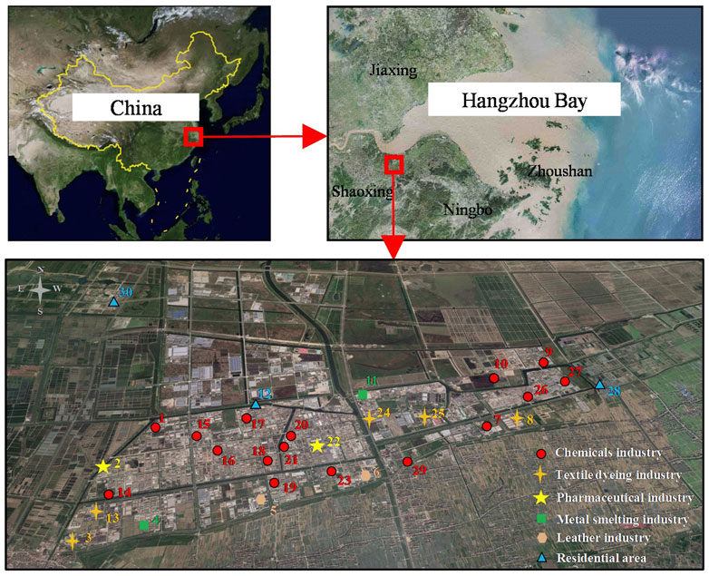
FIGURE 1. Layout of the study area demonstrating locations of the sampling sites (chemicals industry: , Textile dyeing industry: , Pharmaceuticals industry: , Metal smelting industry: , Leather industry: , Residential area: ) (from Google Maps).

Ambient air pollutants had been monitored by 30 AQMSs across the FCIP from December 2019 to November 2020. To investigate the spatial distribution of the pollutants in the area, 30 sampling sites were selected over a grid system based on their different category. These sampling sites were distributed in different industrial enterprises, including the chemicals industry (n = 16), textile dyeing industry (n = 5), pharmaceuticals industry (n = 2), metal smelting industry (n = 2), leather industry (n = 2) and residential area (n = 3), as illustrated in Figure 1.

2.2 Apparatus

In this study, a total of thirty AQMSs based on gas sensors (AQMS-1100, Beijing SDL Technology Co., Ltd., China) were employed. The device is shown in Figure 2. The whole device with a size of 330 × 120 × 230 mm (L×W×H) has a power consumption of 5W over each analytical cycle powered by 12 VDC batteries (Figure 2A). There are two layers in the device, and the lower layer is the installation position of the host, the schematic diagram of the host is shown in Figure 2B. All sensors are housed in the host, through which the calibration gas or sampled air is introduced to the sensor heads under controlled conditions. TVOCs, CO, NO₂, O₃, PM and meteorological parameters are simultaneously monitored. The technical parameters of the sensors are shown in Supplementary Table S1 including accuracy, detection deviation and time resolution. The upper layer is reserved for the installation position of the power supply equipment. The outer part of the cabinet has wind speed (WS) and wind direction (WD) measurement unit. The monitoring data can be recorded and transmitted in real-time. In this study, the sensors were regularly maintained and calibrated monthly by our dedicated maintenance staff as described in the previous study (Pang et al., 2021). If the AQMSs monitoring data shows negative values or if the span exceeds the monitoring limits of the sensor, the data collected at that point will be considered erroneous and will not be used for statistical purposes. Also, if there is a temporary power failure at the AQMSs, the data should be considered invalid from the time of the power failure until power is restored and the instrument has gone through a 24-h warm-up period. In addition, previous experiments have demonstrated that the sensors data agreed well with the reference data, with R² values ranging from 0.81 to 0.93 (Pang et al., 2021).

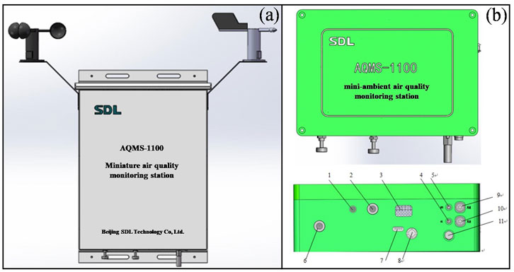
FIGURE 2. The overall appearance of AQMS (A). The host of AQMS (B). the air sensors are installed inside the device host. The interfaces of the device are introduced as the following: 1 air outlet, 2 PMS15 template air inlet, 3 air outlet, 4 4G antenna interface, 5 GPS antenna interface, 6 air inlet of gas monitoring unit, 7 air inlet of PM monitoring unit, 8 air outlet of PM monitoring unit, 9 WS sensor interface, 10 WD sensor interface, 11 temperature and relative humanity (RH) sensors.

2.3 Mapping and pollutants distribution

The natural neighborhood method in the geographic information system (ArcGIS 10.8) was used to map the distribution of air pollutants in the four seasons to assess the spatial distribution of pollutants in FCIP. The mean concentration of individual pollutants at each site during four seasons was used. The sampling periods were divided into December 2019 to February 2020, March to May 2020, Jun to August 2020, and September to November 2020, representing the seasons of winter, spring, summer, and autumn, respectively.

3 Results and discussion

3.1 Temporal variations of air pollutants

Through the established air quality monitoring network, sampling campaigns were performed across four seasons, and the concentrations of TVOCs, CO, NO₂, O₃, PM_2.5, and PM₁₀ were obtained. The temporal variations of air pollutant concentrations during the whole sampling campaign period are presented in Figure 3 and Supplementary Table S2. In general, air pollutants except for TVOCs and O₃ had the highest concentration levels in winter compared to other seasons. The higher concentrations of air pollutants in winter are most plausibly due to the frequent occurrence of inversion layers and lower atmospheric boundary heights (Bozkurt et al., 2018). In Figure 3A, Supplementary Figure S2, TVOCs concentration shows an overall tendency of a single peak, with the highest monthly average concentration in August, with an average concentration of 1978 ppb, as listed in Supplementary Table S2. Generally, TVOCs concentration was higher in summer (1954 ppb) than in winter (1,509 ppb), as the same phenomena were found in other studies (Hoque et al., 2008; Dumanoglu et al., 2014), probably due to increased volatilization of VOCs from organic products at higher ambient temperature (30 ± 4°C) in summer (Supplementary Table S4). However, the temporal distributions of TVOCs at some sampling sites are inconsistent with the above phenomenon, as shown in Figure 4, Supplementary Figure S3. In Figure 4A, TVOCs concentration increased rapidly in March and then fell to its original concentration level after maintaining a stable period. At site 13, the concentration of TVOCs showed an intermittent increase (Figure 4B), which may be related to the daily production output. As shown in Figures 4C,D, at sites 20 and 27, the concentrations of TVOCs decreased sharply in June and November, respectively, and then remained stable. The sudden increase or decrease of TVOCs concentration during the monitoring period could be the result of a change in production mode in industries or a risk of be leakage, providing companies with a basis for appropriate control measures. On the whole, the hourly concentration of TVOCs in FCIP was mainly concentrated in a range between 1,255 and 2,165 ppb accounting for 89.0% of the total range as shown in Supplementary Figure S1A, which were much higher than the concentrations of TVOCs in many urban areas (38.2–67.0 ppb) (Han et al., 2019; Huang et al., 2022; Li et al., 2023).

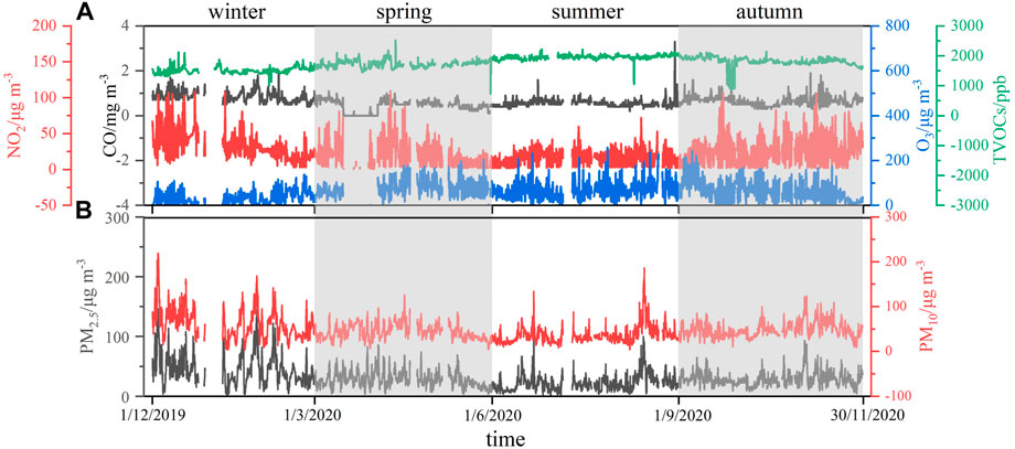
FIGURE 3. Temporal variation of TVOCs, CO, NO₂, and O₃ (A), PM_2.5, and PM₁₀ (B) at station NO1, which represents the general temporal variations of air pollutants in FCIP.

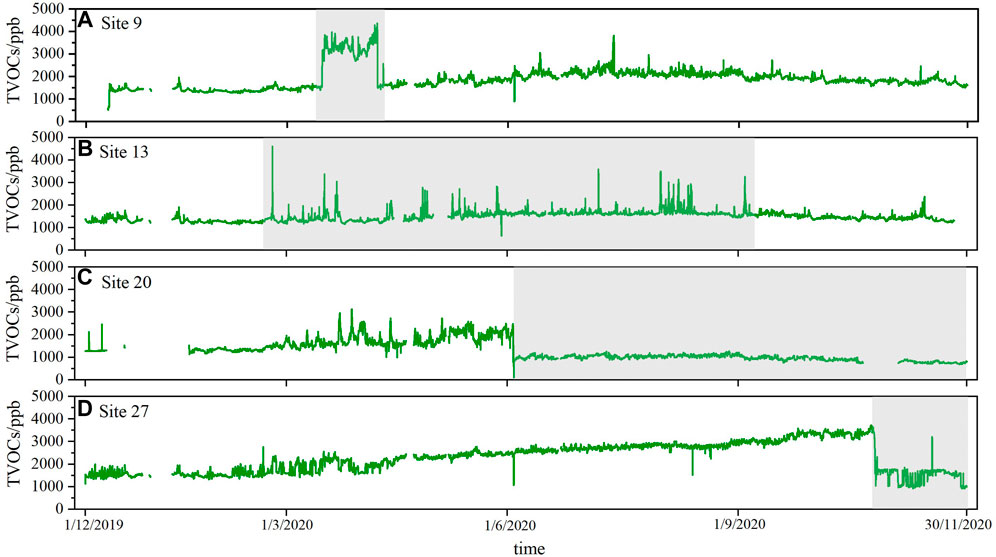
FIGURE 4. Temporal variation of TVOCs at monitoring stations of site 9 (A), site 13 (B), site 20 (C) and site 27 (D), TVOCs concentrations showed a trend of sudden increase or decrease in a certain monitoring period.

Supplementary Figures S4, S5 show the temporal variations of air pollutant concentrations at the three residential sites during the sampling campaign and their correlation with the other source sites in the FCIP (site 12, site 28, site 30). Overall, these three sites had persistently high concentrations of pollutants that undoubtedly posed a risk to people who were permanently exposed to this environment (Supplementary Table S3). Several studies have shown that there is a link between living near industrial complexes and the occurrence of adverse health outcomes (Al-Wahaibi and Zeka 2015; Broitman and Portnov 2020; Marquès et al., 2020). It is worth noting that the trends in pollutant concentrations at these three sites were strongly consistent with the other sources in the park, with R² up to 0.979 (p < 0.01). As with other source sites in the FCIP, the residential sites reached their highest concentrations of TVOCs in the summer season and higher concentrations of CO in the winter. We also found that for a primary pollutant such as CO, sites 12 and 28, which were located near dense facilities, correlate better with the source sites than site 30, which was located farther away. Since we did not have access to the concentrations of the individual VOC species, we cannot provide any further information on the degree of hazard, but it can be inferred that the residents of the industrial park were permanently exposed to pollutant emissions from industrial sources and may be more affected by their primary pollutants closer to the sources. Therefore, we strongly recommend that factories take measures such as changing their processes to significantly reduce air pollution emissions, thereby reducing the risks to human health.

During the monitoring period, the hourly concentrations of O₃ and NO₂ were mainly concentrated in a range between 31 and 79 μg m⁻³ and 4–28 μg m⁻³, which accounted for 62.0% and 72.2% of the whole concentration ranges, respectively (Supplementary Figures S1B,C). Notably, the O₃ concentrations were higher in April (88.8 μg m⁻³) and September (78.5 μg m⁻³) (in spring and early autumn) (Supplementary Table S2), which is more different from the seasonal variation of other pollutants. It might be attributable to the accumulation of pollutants in winter when radiation is lower compared to other seasons, followed by enhanced photochemistry in spring when solar radiation is higher (Fernández-Fernández et al., 2011). And in a monsoon climate, more precipitations lead to lower O₃ concentrations in summer (Yu et al., 2020). By comparison, the lowest O₃ concentration occurred in winter (34.0 μg m⁻³) due to the fact that O₃, as a secondary pollutant, depends heavily on solar compliance and temperature, with weaker sunlight and lower temperatures in winter ultimately inhibiting the formation of O₃ (Zhang et al., 2015; Song et al., 2022).

The concentration of CO was relatively low in spring and summer and high in winter (Figure 3, Supplementary Table S2). This is explained by the fact that the photochemistry of CO almost disappears in winter, mainly due to the direct influence of anthropogenic activities, and CO concentrations are increased by continuous emissions from factories in winter (Koike et al., 2006). Whereas, photochemistry is greater in spring and summer and the emitted CO is dispersed by OH radicals, additionally to stronger convection and good diffusion in summer and autumn, which also leads to relatively low CO concentrations in the atmosphere (Li et al., 2019). As can be seen in Figure 3B, the concentrations of PM₁₀ and PM_2.5 have a good consistent trend, which reflects the similarity of the two sources. The concentrations of PM_2.5 covered a range between 16 and 46 μg m⁻³ accounting for 72.4% of the total concentration range (Supplementary Figure S1E)., indicating that the concentration of PM_2.5 in the atmosphere of the industrial park was basically in line with the national air quality standards (75 μg m⁻³). VOCs as the important precursors of secondary PM_2.5 showed a negative correlation to PM_2.5 (Supplementary Table S2) (Chen et al., 2017), PM_2.5 concentrations were higher in winter and lower in summer, which was opposite to the trend of TVOCs concentration, above phenomenon was contrary to some other studies (Han et al., 2017; Li et al., 2020). However, this is similar to CO and could be attributed to the fact that PM accumulates less during the summer monsoon when dispersion conditions are good, which ultimately leads to low PM concentrations in the summer (Tian et al., 2020).

In addition, a comparison of monitoring results from the FCIP with those from the urban region reveals a consistent overall trend in Supplementary Table S5, but with the exception of O₃, the lowest concentrations in the FCIP appear primarily in May and July, while in the urban region they appear in July and August. Interestingly, the FCIP has significantly higher NO₂ and PM concentrations in December and November than the urban region, while concentrations in the FCIP are lower in the other months.

3.2 Spatial variation of air pollutants

Mapping was performed with the seasonal mean values of the whole sampling campaigns at each sampling site. Spatial distribution maps of TVOCs and air pollutants are prepared to interpolate their concentrations measured at 29 sites by the GIS software, shown in Figure 5 and Figure 6. The site excluded was located outside the FCIP as the background site.

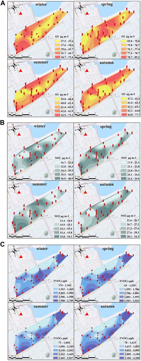
FIGURE 5. Spatial distribution of O₃ (A), NO₂ (B), and TVOCs (C) from December 2019 to November 2020, including 29 air monitoring stations in FCIP. One site is not included because it is located outside the FCIP (the red triangle represents that site).

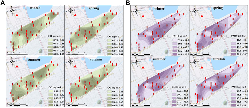
FIGURE 6. Spatial distribution of CO (A), PM₁₀ (B) from December 2019 to November 2020, including 29 air monitoring stations in FCIP. One site is not included because it is located outside the FCIP (the red triangle represents that site).

As seen in Figure 5, the spatial distributions of TVOCs, NO₂ and O₃ have a significant negative correlation and the concentrations of TVOCs and NO₂ were lower in the area with high O₃ concentration, which indicated that the atmospheric photochemical reaction of O₃ was significantly affected by local pollutants in the pollution process. In FCIP, TVOCs and NO₂ emitted by transportation and industries were the main sources of O₃ concentrations as the main precursors of O₃. NO₂ produces NO and O atoms through photolysis and then O atoms react with O₂ to produce O₃. In addition, NO reacts with O₃ to produce NO₂ and O₂. Through the above reaction, a dynamic equilibrium is formed between NO₂ and O₃. When VOCs exist in the atmosphere, hydroxyl radical (OH) reacts with active VOCs to produce organic radicals (R). R combines with O₂ to produce RO₂·, which will react with NO to consume NO and produce NO₂, thus breaking the dynamic equilibrium between NO₂ and O₃ and increasing the concentration of O₃.

The area is NO₂-limited for the O₃ formation if the ratio between VOCs and NO₂ concentration is higher than 8, otherwise, that is VOCs-limited (Mozaffar et al., 2020). In this study, the ratios were higher than 8 in four seasons, and O₃ formation was more sensitive to the NO₂ concentrations than the VOCs concentrations. Under this circumstance, the efficient strategy to reduce O₃ formation rates will be the reduction of NO₂ concentration in the air. NO₂ concentrations were higher in the middle region of FCIP (Figure 5B), which provides direction for FCIP to reduce NO₂ pollution. Based on the in-situ survey, the area has a long history of emissions from heavy-duty trucks, which in turn contain a large amount of NO_x, thus increased traffic control in the area can be effective in reducing NO_x and VOCs (Ximinis et al., 2021). In Figure 5C, it was noteworthy that TVOCs concentration was higher in the middle and southeast region of the FCIP in four seasons. But the highest concentration of TVOCs was site 27 in the northeast corner (geographical position shown in Figure 1), which also results in generally higher concentrations at site 28 and has a significant impact on the residents living there. The spatial distribution patterns of CO and PM₁₀ were obtained and shown in Figure 6. Although concentrations of species varied seasonally, the distribution patterns were not significantly different. It is interesting to note that higher CO and PM₁₀ concentrations are also observed in the intermediate area of the FCIP (Figure 6), as they are primary pollutants that are probably emitted directly from the surrounding intensive chemical factories and complex production processes in this region.

3.3 Pollutant emissions analysis of different industries

The FCIP is dotted with all types of factories, but the sampling sites can be divided into five main categories depending on the industrial categories and the residential area. The mean concentrations of pollutants for each category are given in Table 1. The highest atmospheric TVOCs concentrations were observed in the textile dyeing industry (3,088.9 ± 1,507.7 ppb), followed by the pharmaceuticals industry (2,192.3 ± 368.4 ppb). It’s related to the fact that VOCs emission from the textile dyeing and pharmaceutical industries was characterized by great intermittent and fugitive emissions from many leakage sites in producing processes, resulting in higher concentrations of pollutants in the atmosphere (Hou et al., 2020; Khattab et al., 2020; Zhou et al., 2020; Cheng et al., 2021). Moreover, the concentrations of NO₂ were very similar in the different industrial categories, but significantly higher concentrations were measured in the pharmaceutical industry, with an annual mean of 28.3 ± 13.6 μg m⁻³ (Table 1), so that further study of the pharmaceutical industry in terms of NO₂ characteristics could be conducted to effectively reduce pollution. O₃ concentrations reached the highest levels in the textile dyeing industry with an annual average O₃ concentration was 62.6 ± 18.1 μg m⁻³ (Table 1), which can be attributed to the fact that the concentrations of O₃ as a secondary pollutant are strongly influenced by its precursors (NO₂ and VOCs) and the textile printing and dyeing industry emitted far more TVOCs. Although none of the precursors (VOCs and NO₂) were as high as in the pharmaceutical industry, the leather industry was second only to the textile printing and dyeing industry in O₃ concentrations, likely related to more species with high ozone formation potential in the VOCs emitted by the leather industry. The environmental background value of CO is relatively high with longer lifetime. In FCIP, CO concentration was found to be slightly higher in the pharmaceuticals industry (0.66 ± 0.16 μg m⁻³) and textile dyeing industry (0.65 ± 0.18 μg m⁻³) than in other industrial categories. In FCIP, the high concentrations of PM in the metal smelting industry are noteworthy, which was similar to the results reported in other studies (Wei et al., 2019). It has been shown by studies that almost every stage of the metal smelting process produces PM, including organic carbon, black carbon, and heavy and trace metals, all of which are the main components of PM in the atmosphere (Owoade et al., 2015). Therefore, it is urged that the metal smelting industry should focus on reducing PM as a priority measure to decrease pollution. Taken together, the textile dyeing and pharmaceuticals industries were the enterprises with serious air pollution in FCIP and their emissions polluted the living areas nearby to some extent.

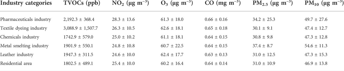
TABLE 1. The annual mean values of air pollutants in different industries were calculated.

3.4 Diurnal variation characteristics of O₃, TVOCs and NO₂

As the most concerned pollutant, VOCs have an important influence on O₃ formation (Xing et al., 2011). Hence, the influence rule of VOCs on O₃ was further discussed, together with NO₂ as another precursor of O₃. As shown in Figure 7A and Figure 8C, the winter and summer average statistics of the monitoring data were carried out by each other. The diurnal variation of O₃ concentration showed a distinct unimodal pattern, reaching its maximum at 15:00 LT, which was about 1 h later than the peak of O₃ in Tianjin and Guangzhou (Zou et al., 2015; Liu et al., 2016), but consistent with the time of O₃ peak in cities such as Beijing and Shandong (Wang et al., 2015; Zhang et al., 2019). Due to the complex generation mechanisms of O₃ (VOCs and NO₂-limited), the above phenomena may be related to local VOCs and NO₂ emissions and solar radiation. Besides, NO₂ and TVOCs showed bimodal variation. To further understand the O₃, NO₂, and TVOCs concentration change in FCIP, we analyzed the daily change rate of O₃ and its precursors. The calculation is as followed (Liu et al., 2016),

Where, ${\left[\mathrm{X}\right]}_{\mathrm{t}}$ represents the concentrations of O₃, NO₂, and TVOCs at time t, and ${\left[\mathrm{X}\right]}_{\mathrm{t}+1}$ represents the concentration of O₃, NO₂, and TVOCs 1 hour after time t.

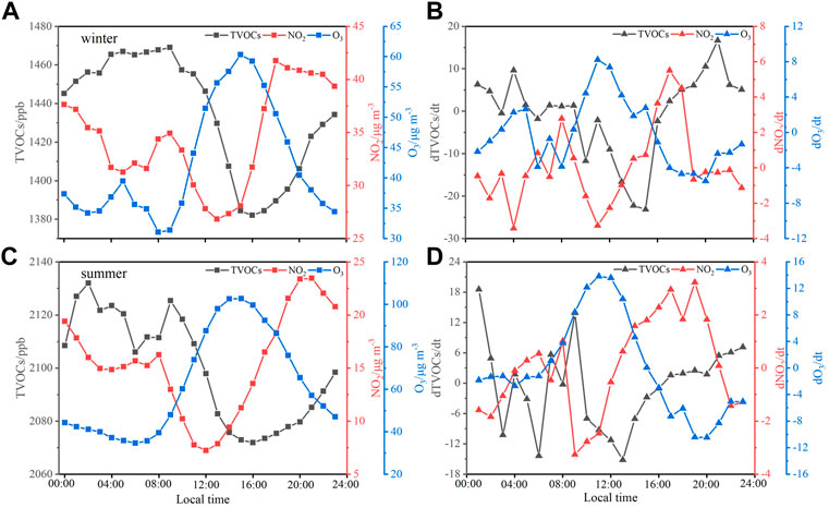
FIGURE 7. The diurnal variations ((A) summer, (C) winter) and change rate ((B) summer, (D) winter) of O₃, TVOCs, and NO₂ during summer and winter in FCIP.

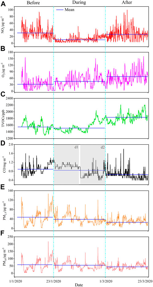
FIGURE 8. Concentration distribution of NO₂ (A), O₃ (B), TVOCs (C), CO (D), PM2.5 (E) PM10 (F) before, during and after the epidemic in a chemical industrial park.

The timely variation rate of O₃ and its precursors were shown in Figures 7B, 8D. The negative variation rate of O₃ concentration indicates that the chemical loss dominates the change, while the positive rate of change in O₃ concentration indicates that the photochemical production of O₃ plays a key role (Zou et al., 2015). Averagely, the negative change rate of O₃ concentration occurred after 16:00 LT. At this time, the sunlight and photochemical reaction began to decrease, resulting in the decrease of OH radicals. After that, because sunlight abated and finally disappeared, OH radical stopped producing, while NO₂ titration continued to consume O₃. During the night in winter, the concentration of O₃ appeared as a weaker peak. This may be caused by vertical O₃ transportation in the stratosphere or accumulation of O₃ due to the low boundary-layer height at night (Cheung and Wang 2001). From 00:00 to 07:00 LT in summer, the variation rate was relatively stable and slightly negative. Due to diffusion of the atmospheric boundary layer and increased photochemistry, the concentration of O₃ showed a positive change rate after 07:00 and reached a peak at approximately 11:00.

The trends of O₃, NO₂, and TVOCs were significantly negatively correlated, and the diurnal variations of TVOCs and NO₂ were bimodal (Figures 7A,C). The concentration of TVOCs showed an obvious increase in the early morning due to human activity (e.g., factory emissions, vehicle exhaust, etc.) and plant emission, reaching a peak at 09:00. Then it gradually decreased and reached the lowest value at 16:00 LT, which may be caused by the synergistic effect of strong photochemical reaction of OH and diffusion. The lowering of the mixed boundary layer in the evening again lead to an increase in TVOCs pollutants. Variations in NO₂ were similar to TVOCs, with peak concentrations occurring between 08:00 and 09:00. A negative rate of change in NO₂ followed from 09:00 as a result of O₃ production and continued NO₂ consumption, with concentrations decreasing rapidly. The pollutant accumulated after the evening traffic peak, with a peak around 19:00 to 20:00. In general, the increase in daytime O₃ concentrations is due to photochemical production of O₃ from its precursors, so the trend in ozone changes is unimodal, in contrast to TVOCs and NO₂.

3.5 Correlation between air pollutants and meteorological conditions

The concentrations of TVOCs, CO, NO₂, O₃, PM_2.5, PM₁₀ and meteorological parameters were counted separately by season, and the correlation analysis between pollutants and temperature, RH, WS was carried out. Supplementary Figure S6 showed the statistics of meteorological conditions for each season at the sites during the observation period. Except for summer, the prevailing wind directions of observation sites were southeast, whereas the dominant wind direction in summer was southeast and southwest. During the different seasons the average WS remained close to 1.7 m s⁻¹, while the average temperature ranged from 11°C in winter to 30°C in summer (Supplementary Table S4).

The relationship between pollutants and meteorological factors was quantified using Pearson correlation coefficient as shown in Table 2. The correlations between all pollutant concentrations and the temperature, RH and WS throughout the year were calculated. PM_2.5, PM₁₀, CO and NO₂ were negatively correlated with WS in all seasons except winter, which indicates horizontal dispersion plays an important role in modulating their concentrations. The concentrations of PM_2.5, PM₁₀, CO and NO₂ positively correlated with RH in all seasons. High RH favors the partition of semi-volatile species into the aerosol phase leading to high PM concentrations (Zhang et al., 2015). Moister atmosphere normally accompanies lower boundary layer further enhancing the concentrations of primary pollutants (Sandeep et al., 2014). The O₃ showed positive correlations with WS in all seasons, which indicated WS promoted O₃ formation through long transportation (Mohamad Nazir et al., 2020). The positive correlations with air temperatures in all seasons implied high air temperature helped the ambient O₃ formation (Wang et al., 2015). The RH had negative correlations with O₃ in all seasons.

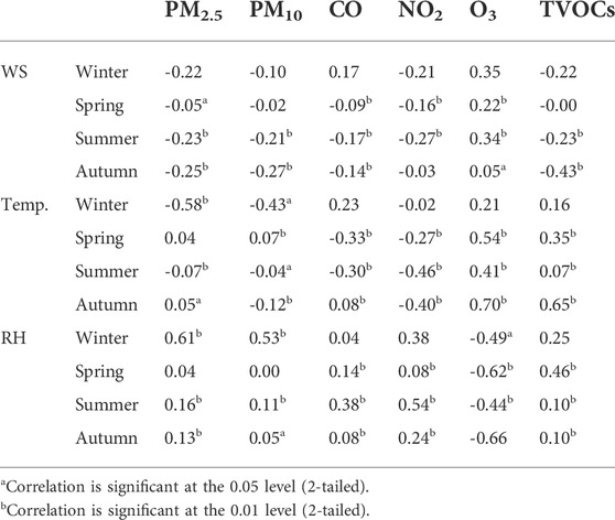
TABLE 2. Summary of pearson correlation coefficient values between air pollutants and temperature, RH and WS.

3.6 Impact of the COVID-19 outbreak on the air pollutants concentration levels

Several cases of “unknown viral pneumonia” were first reported in Wuhan, China, in December 2019, identified in January 2020, and subsequently designated as COVID-19 (Zhang., Li. et al., 2021). Local governments imposed a strict citywide lockdown since the end of January 2020, with many factories closed and road traffic restricted. With the outbreak under control, Shaoxing gradually lifted its blockade measures from late February. Figure 8 shows the variations of concentrations of NO₂, O₃, TVOCs, CO, PM_2.5, and PM₁₀ in a chemical park in Shaoxing City before (January 1, 2020 to January 22, 2020), during (January 23, 2020 to March 1, 2020), and after (March 2, 2020 to March 23, 2020) the outbreak. As shown in Figure 8A, NO₂ concentrations decreased significantly during the epidemic period due to the slowdown of plant transportation and production. After the epidemic, the average TVOCs concentration was up to 1821 ppb (Figure 8C), which was directly related to the increase in TVOCs emissions from the factories after the resumption of work and production in the chemical park. On days 1 through 14 of the outbreak periods, the mean CO concentrations were higher (Figure 8d1), background CO levels were high, and CO had a longer lifetime than NO₂. During the epidemic period from February 5 to March 1, mean CO concentrations were lower (Figure 8d2), reflecting the continued decline in CO emissions resulting from the epidemic. There was a trend for PM_2.5 similar to PM₁₀ (Figures 8E,F), and airborne PM concentrations are mainly influenced by meteorological conditions. The significant decreased in PM after the epidemic period may be due to increased air turbulence from rising temperatures and the improved ability of air to dilute pollutants. It is noteworthy that O₃ concentrations increased during the epidemic period due to a decrease in the concentration of anthropogenic NO₂ emissions from the chemical park during the epidemic period, and the decreased NO concentration slowed the rate of O₃ degradation, resulting in an increase in O₃ concentrations (Figure 8B). In addition, the formation of O₃ in the environment is mainly influenced by NO_x, VOCs concentrations, and gas phase parameters, causing O₃ concentrations to continue to increase after the epidemic period.

In general, NO₂, TVOCs, CO, PM_2.5, and PM₁₀ concentrations were lower on a mean basis during the epidemic than before the epidemic due to the slowdown of production and transport in epidemic factories, while O3 concentrations were higher during the epidemic than before the epidemic on account of their precursors.

4 Conclusion

A 1-year field campaign had firstly been conducted in a typical chemical industrial park in Yangtz River Delta, China from December 2019 to November 2020 based on thirty miniature AQMSs and the concentrations of TVOCs, PM, NO₂, O₃ and CO as well as meteorological conditions were continuously measured. The observations showed that NO₂, CO and PM concentrations were higher in winter than that in other seasons. Such a seasonal variation was likely partly due to the seasonal variation of the atmospheric boundary layer. The concentration of TVOCs was higher in summer due to increased volatilization from their sources at high temperatures. The hourly concentration of TVOCs varied between 1,255 and 2,165 ppb which accounted for 89.0%. During the monitoring period, the concentrations of TVOCs at some sampling sites suddenly decreased or increased, which may be related to production modes and the existence of leakage. Sites in residential areas were significantly correlated with sites from other industrial sources, therefore it is strongly recommended that the factories improve their processes to reduce the health impact on nearby residents. The peak values of O₃ concentration occurred in April (88.8 μg m⁻³) and September (78.5 μg m⁻³) (in spring and early autumn) due to the summer monsoon climate more precipitations lead to lower O₃ concentration in summer. We found similar seasonal variations for CO and particulate matter, which also suggests that good convective diffuse conditions can reduce pollution. The O₃ concentration was higher in the area with low TVOCs and NO₂ concentrations, which indicated that the spatial distributions of O₃ and its precursors had a significant negative correlation and the formation of O₃ was significantly affected by local pollutants in the pollution process. Based on the ratio of NO₂ to TVOCs, it was also determined that the FCIP was in the NO₂-limited region during the monitoring period and that an effective strategy to reduce O₃ formation was to lower the NO₂ concentration in the air. The analysis of pollutant emissions from different industries showed that O₃ pollution was more serious in t textile dyeing industry, NO₂ emissions were more serious in the pharmaceutical industry, and the reduction of PM pollution must focus on the metal smelting industry.

The daily change of O₃ concentration reached its peak at 15:00 LT and appeared a weaker peak during the night in winter which may be caused by vertical O₃ transportation and low boundary layer height. The trends of O₃ precursors (TVOCs and NO₂) were clearly negatively correlated with O₃ and showed a bimodal peak due to anthropogenic activities, plant emissions, lowering of the mixed boundary layer, etc. In particular, it was found that high relative humidity favored the entry of semi-volatiles into the aerosol phase, resulting in high PM concentrations, and that WS with high temperatures contributed to the formation of O₃ in the environment.

This study generates important information and methods for the study of air pollutant characteristics in FCIP, suggesting the need to focus research on different pollutants for different industries to further reduce the health impacts on the surrounding residents. Further analysis based on the time of epidemic prevention and control revealed that O₃ concentrations were higher during the epidemic than before the epidemic due to its precursors, while other pollutants were affected by the slowdown in production and transportation of epidemic plants, and their mean concentrations were lower during the epidemic than before the epidemic. In conclusion, the grid-based monitoring research of FCIP is essential for formulating emission control strategies, recognizing the impact of pollution sources, and supporting the related applications of government, local institutions, and enterprises.

Data availability statement

The raw data supporting the conclusions of this article will be made available by the authors, without undue reservation.

Author contributions

XP: Conceptualization, Writing-review and editing, Funding acquisition. YL: Conceptualization, Formal analysis, Writing-original draft. BW: Project administration, Funding acquisition. HW: Writing-review and editing, Supervision. KS: Conceptualization, Formal analysis, Methodology, Writing-original draft. JL: Investigation, Visualization. BX: Supervision. LC: Data curation. ZW: Investigation, Data curation. SD: Investigation. WZ: Software. XC: Software. DC: Writing-review and editing, Supervision. JC: Supervision.

Funding

This work was supported by National Key R&D Program of China (2021YFF0600202), National Natural Science Foundation of China (41727805), Zhejiang Province “Lingyan” Research and Development Project (2022C03073), the Natural Science Foundation of Zhejiang Province, China (LZ20D050002), Key Research Program of Zhejiang Province (2021C03165), Key project of Scientific and Technological Research Program of Chongqing Municipal Education Commission (KJZD-M202201402 and KJZD-K201901403) and General project of Natural Science Foundation of Chongqing Bureau of science and technology (cstc2019jcyj-msxmX0879).

Conflict of interest

Authors WZ and XC are employed by Beijing SDL Technology Co.

The remaining authors declare that the research was conducted in the absence of any commercial or financial relationships that could be construed as a potential conflict of interest.

Publisher’s note

All claims expressed in this article are solely those of the authors and do not necessarily represent those of their affiliated organizations, or those of the publisher, the editors and the reviewers. Any product that may be evaluated in this article, or claim that may be made by its manufacturer, is not guaranteed or endorsed by the publisher.

Supplementary material

The Supplementary Material for this article can be found online at: https://www.frontiersin.org/articles/10.3389/fenvs.2022.1026842/full#supplementary-material

References

Al-Wahaibi, A., and Zeka, A. (2015). Health impacts from living near a major industrial park in Oman. BMC Public Health 15, 524. doi:10.1186/s12889-015-1866-3
An, Z., Wang, N., Bai, D., Yu, X., and Liu, S. (2021). The enlightenment on emergency management of chemical parks. IOP Conf. Ser. Earth Environ. Sci. 791, 012181. doi:10.1088/1755-1315/791/1/012181
Baek, K.-M., Kim, M.-J., Kim, J.-Y., Seo, Y.-K., and Baek, S.-O. (2020). Characterization and health impact assessment of hazardous air pollutants in residential areas near a large iron-steel industrial complex in Korea. Atmos. Pollut. Res. 11, 1754–1766. doi:10.1016/j.apr.2020.07.009
Borrego, C., Ginja, J., Coutinho, M., Ribeiro, C., Karatzas, K., Sioumis, T., et al. (2018). Assessment of air quality microsensors versus reference methods: The EuNetAir Joint Exercise – Part II. Atmos. Environ. 193, 127–142. doi:10.1016/j.atmosenv.2018.08.028
Bozkurt, Z., Üzmez, Ö. Ö., Döğeroğlu, T., Artun, G., and Gaga, E. O. (2018). Atmospheric concentrations of SO2, NO2, ozone and VOCs in Düzce, Turkey using passive air samplers: Sources, spatial and seasonal variations and health risk estimation. Atmos. Pollut. Res. 9, 1146–1156. doi:10.1016/j.apr.2018.05.001
Broitman, D., and Portnov, B. A. (2020). Forecasting health effects potentially associated with the relocation of a major air pollution source. Environ. Res. 182, 109088. doi:10.1016/j.envres.2019.109088
Chen, C., Chuang, Y., Hsieh, C., and Lee, C. (2019). VOC characteristics and source apportionment at a PAMS site near an industrial complex in central Taiwan. Atmos. Pollut. Res. 10, 1060–1074. doi:10.1016/j.apr.2019.01.014
Chen, L., and Pang, X. (2020). Photo-ionization sensors as detectors in GC×GC systems for ambient VOCs measurements. Ecolo. Environ. Monit. Three Gorges 5, 62–70. doi:10.19478/j.cnki.2096-2347.2020.03.07
Chen, Q., Fu, T., Hu, J., Ying, Q., and Zhang, L. (2017). Modelling secondary organic aerosols in China. Natl. Sci. Rev. 4, 806–809. doi:10.1093/nsr/nwx143
Cheng, N., Jing, D., Zhang, C., Chen, Z., Li, W., Li, S., et al. (2021). Process-based VOCs source profiles and contributions to ozone formation and carcinogenic risk in a typical chemical synthesis pharmaceutical industry in China. Sci. Total Environ. 752, 141899. doi:10.1016/j.scitotenv.2020.141899
Cheung, V. T. F., and Wang, T. (2001). Observational study of ozone pollution at a rural site in the Yangtze Delta of China. Atmos. Environ. 35, 4947–4958. doi:10.1016/s1352-2310(01)00351-x
Dumanoglu, Y., Kara, M., Altiok, H., Odabasi, M., Elbir, T., and Bayram, A. (2014). Spatial and seasonal variation and source apportionment of volatile organic compounds (VOCs) in a heavily industrialized region. Atmos. Environ. 98, 168–178. doi:10.1016/j.atmosenv.2014.08.048
Fernández-Fernández, M. I., Gallego, M. C., García, J. A., and Acero, F. J. (2011). A study of surface ozone variability over the Iberian Peninsula during the last fifty years. Atmos. Environ. 45, 1946–1959. doi:10.1016/j.atmosenv.2011.01.027
Han, C., Liu, R., Luo, H., Li, G., Ma, S., Chen, J., et al. (2019). Pollution profiles of volatile organic compounds from different urban functional areas in Guangzhou China based on GC/MS and PTR-TOF-MS: Atmospheric environmental implications. Atmos. Environ. 214, 116843. doi:10.1016/j.atmosenv.2019.116843
Han, D., Wang, Z., Cheng, J., Wang, Q., Chen, X., and Wang, H. (2017). Volatile organic compounds (VOCs) during non-haze and haze days in shanghai: Characterization and secondary organic aerosol (SOA) formation. Environ. Sci. Pollut. Res. 24, 18619–18629. doi:10.1007/s11356-017-9433-3
Hoque, R. R., Khillare, P. S., Agarwal, T., Shridhar, V., and Balachandran, S. (2008). Spatial and temporal variation of BTEX in the urban atmosphere of Delhi, India. Sci. Total Environ. 392, 30–40. doi:10.1016/j.scitotenv.2007.08.036
Hou, X., Guo, B., and Ren, T. (2020). Performance evaluation methods and effect analysis of VOCs-related enterprises in key industries. IOP Conf. Ser. Earth Environ. Sci. 474, 052062. doi:10.1088/1755-1315/474/5/052062
Huang, H., Wang, Z., Guo, J., Wang, C., and Zhang, X. (2022). Composition, seasonal variation and sources attribution of volatile organic compounds in urban air in southwestern China. Urban Clim. 45, 101241. doi:10.1016/j.uclim.2022.101241
Jia, H., Gao, S., Duan, Y., Fu, Q., Che, X., Xu, H., et al. (2021). Investigation of health risk assessment and odor pollution of volatile organic compounds from industrial activities in the Yangtze River Delta region, China. Ecotoxicol. Environ. Saf. 208, 111474. doi:10.1016/j.ecoenv.2020.111474
Khattab, T. A., Abdelrahman, M. S., and Rehan, M. (2020). Textile dyeing industry: Environmental impacts and remediation. Environ. Sci. Pollut. Res. 27, 3803–3818. doi:10.1007/s11356-019-07137-z
Koike, M., Jones, N. B., Palmer, P. I., Matsui, H., Zhao, Y., Kondo, Y., et al. (2006). Seasonal variation of carbon monoxide in northern Japan: Fourier transform IR measurements and source-labeled model calculations. J. Geophys. Res. 111, D15306. doi:10.1029/2005JD006643
Kumar, P., Morawska, L., Martani, C., Biskos, G., Neophytou, M., Di Sabatino, S., et al. (2015). The rise of low-cost sensing for managing air pollution in cities. Environ. Int. 75, 199–205. doi:10.1016/j.envint.2014.11.019
Li, B., Ho, S. S. H., Li, X., Guo, L., Feng, R., and Fang, X. (2023). Pioneering observation of atmospheric volatile organic compounds in Hangzhou in eastern China and implications for upcoming 2022 Asian Games. J. Environ. Sci. 124, 723–734. doi:10.1016/j.jes.2021.12.029
Li, B., Yang, L., and Tang, S. H. (2019). Intraseasonal variations of summer convection over the Tibetan Plateau revealed by geostationary satellite FY-2E in 2010-14. J. Meteorol. Res. 33, 478–490. doi:10.1007/s13351-019-8610-3
Li, Q., Su, G., Li, C., Liu, P., Zhao, X., Zhang, C., et al. (2020). An investigation into the role of VOCs in SOA and ozone production in Beijing, China. Sci. Total Environ. 720, 137536. doi:10.1016/j.scitotenv.2020.137536
Lin, Y. C., Lai, C. Y., and Chu, C. P. (2021). Air pollution diffusion simulation and seasonal spatial risk analysis for industrial areas. Environ. Res. 194, 110693. doi:10.1016/j.envres.2020.110693
Liu, B., Liang, D., Yang, J., Dai, Q., Bi, X., Feng, Y., et al. (2016). Characterization and source apportionment of volatile organic compounds based on 1-year of observational data in Tianjin, China. Environ. Pollut. 218, 757–769. doi:10.1016/j.envpol.2016.07.072
Marquès, M., Domingo, J. L., Nadal, M., and Schuhmacher, M. (2020). Health risks for the population living near petrochemical industrial complexes. 2. Adverse health outcomes other than cancer. Sci. Total Environ. 730, 139122. doi:10.1016/j.scitotenv.2020.139122
Mohamad Nazir, A. U., Awang, N. R., Ramli, N. A., Daliman, S., and Aziz, H. A. (2020). Effect of monsoonal period toward night-time ground level ozone in East Coast Malaysia. IOP Conf. Ser. Earth Environ. Sci. 549, 012003. doi:10.1088/1755-1315/549/1/012003
Mozaffar, A., Zhang, Y.-L., Fan, M., Cao, F., and Lin, Y.-C. (2020). Characteristics of summertime ambient VOCs and their contributions to O3 and SOA formation in a suburban area of Nanjing, China. Atmos. Res. 240, 104923. doi:10.1016/j.atmosres.2020.104923
Owoade, K. O., Hopke, P. K., Olise, F. S., Ogundele, L. T., Fawole, O. G., Olaniyi, B. H., et al. (2015). Chemical compositions and source identification of particulate matter (PM2.5 and PM2.5–10) from a scrap iron and steel smelting industry along the Ife–Ibadan highway, Nigeria. Atmos. Pollut. Res. 6, 107–119. doi:10.5094/APR.2015.013
Pang, X., Chen, L., Shi, K., Wu, F., Chen, J., Fang, S., et al. (2021). A lightweight low-cost and multipollutant sensor package for aerial observations of air pollutants in atmospheric boundary layer. Sci. Total Environ. 764, 142828. doi:10.1016/j.scitotenv.2020.142828
Pang, X., Nan, H., Zhong, J., Ye, D., Shaw, M. D., and Lewis, A. C. (2019). Low-cost photoionization sensors as detectors in GC × GC systems designed for ambient VOC measurements. Sci. Total Environ. 664, 771–779. doi:10.1016/j.scitotenv.2019.01.348
Pascal, M., Pascal, L., Bidondo, M. L., Cochet, A., Sarter, H., Stempfelet, M., et al. (2013). A review of the epidemiological methods used to investigate the health impacts of air pollution around major industrial areas. J. Environ. Public Health 2013, 1–17. doi:10.1155/2013/737926
Piedrahita, R., Xiang, Y., Masson, N., Ortega, J., Collier, A., Jiang, Y., et al. (2014). The next generation of low-cost personal air quality sensors for quantitative exposure monitoring. Atmos. Meas. Tech. 7, 3325–3336. doi:10.5194/amt-7-3325-2014
Sandeep, A., Rao, T. N., Ramkiran, C. N., and Rao, S. V. B. (2014). Differences in atmospheric boundary-layer characteristics between wet and dry episodes of the indian summer monsoon. Bound. Layer. Meteorol. 153, 217–236. doi:10.1007/s10546-014-9945-z
Schneider, P., Castell, N., Vogt, M., Dauge, F. R., Lahoz, W. A., and Bartonova, A. (2017). Mapping urban air quality in near real-time using observations from low-cost sensors and model information. Environ. Int. 106, 234–247. doi:10.1016/j.envint.2017.05.005
Song, Y., Zhang, Y., Liu, J., Zhang, C., Liu, C., Liu, P., et al. (2022). Rural vehicle emission as an important driver for the variations of summertime tropospheric ozone in the Beijing-Tianjin-Hebei region during 2014–2019. J. Environ. Sci. 114, 126–135. doi:10.1016/j.jes.2021.08.015
Spinelle, L., Gerboles, M., Villani, M. G., Aleixandre, M., and Bonavitacola, F. (2015). Field calibration of a cluster of low-cost available sensors for air quality monitoring. Part A: Ozone and nitrogen dioxide. Sensors Actuators B Chem. 215, 249–257. doi:10.1016/j.snb.2015.03.031
Tian, J., Fang, C., Qiu, J., and Wang, J. (2020). Analysis of pollution characteristics and influencing factors of main pollutants in the atmosphere of Shenyang City. Atmosphere 11, 766. doi:10.3390/atmos11070766
Wang, X., Lei, Y., Yan, L., Liu, T., Zhang, Q., and He, K. (2019). A unit-based emission inventory of SO2, NOx and PM for the Chinese iron and steel industry from 2010 to 2015. Sci. Total Environ. 676, 18–30. doi:10.1016/j.scitotenv.2019.04.241
Wang, Z., Li, Y., Chen, T., Zhang, D., Sun, F., Wei, Q., et al. (2015). Ground-level ozone in urban Beijing over a 1-year period: Temporal variations and relationship to atmospheric oxidation. Atmos. Res. 164-165, 110–117. doi:10.1016/j.atmosres.2015.05.005
Wei, Z., Wang, L. T., Hou, L. Q., Zhang, H. M., Yue, L., Wei, W., et al. (2019). “Source apportionment of PM2.5 in Handan City, China using a combined method of receptor model and chemical transport model,” in Sustainable development of water resources and hydraulic engineering in China. Switzerland: Springer Cham, 151–173.
Wu, F., Zhu, G., Yu, Y., and Sun, J. (2021). Safety risks and countermeasures of chemical industry park in Jiangsu Province. IOP Conf. Ser. Earth Environ. Sci. 680, 012124. doi:10.1088/1755-1315/680/1/012124
Ximinis, J., Massaguer, A., Pujol, T., and Massaguer, E. (2021). Nox emissions reduction analysis in a diesel Euro VI Heavy Duty vehicle using a thermoelectric generator and an exhaust heater. Fuel 301, 121029. doi:10.1016/j.fuel.2021.121029
Xing, J., Wang, S. X., Jang, C., Zhu, Y., and Hao, J. M. (2011). Nonlinear response of ozone to precursor emission changes in China: A modeling study using response surface methodology. Atmos. Chem. Phys. 11, 5027–5044. doi:10.5194/acp-11-5027-2011
Yu, S., Yin, S., Zhang, R., Wang, L., Su, F., Zhang, Y., et al. (2020). Spatiotemporal characterization and regional contributions of O3 and NO2: An investigation of two years of monitoring data in Henan, China. J. Environ. Sci. 90, 29–40. doi:10.1016/j.jes.2019.10.012
Zhang, H., Wang, Y., Hu, J., Ying, Q., and Hu, X. M. (2015). Relationships between meteorological parameters and criteria air pollutants in three megacities in China. Environ. Res. 140, 242–254. doi:10.1016/j.envres.2015.04.004
Zhang, J., Wang, C., Qu, K., Ding, J., Shang, Y., Liu, H., et al. (2019). Characteristics of ozone pollution, regional distribution and causes during 2014–2018 in Shandong Province, east China. Atmosphere 10, 501. doi:10.3390/atmos10090501
Zhang T, T., Xiao, S., Wang, X., Zhang, Y., Pei, C., Chen, D., et al. (2021). Volatile organic compoundsmonitored online at three photochemical assessment monitoring stations in the pearl river delta (PRD) region during summer 2016: Sources and emission areas. Atmosphere 12, 327. doi:10.3390/atmos12030327
Zhang, X., Gao, S., Fu, Q., Han, D., Chen, X., Fu, S., et al. (2020). Impact of VOCs emission from iron and steel industry on regional O3 and PM2.5 pollutions. Environ. Sci. Pollut. Res. 27, 28853–28866. doi:10.1007/s11356-020-09218-w
Zheng, H., Kong, S., Yan, Y., Chen, N., Yao, L., Liu, X., et al. (2020). Compositions, sources and health risks of ambient volatile organic compounds (VOCs) at a petrochemical industrial park along the Yangtze River. Sci. Total Environ. 703, 135505. doi:10.1016/j.scitotenv.2019.135505
Zhou, L., Ma, C., Horlyck, J., Liu, R., and Yun, J. (2020). Development of pharmaceutical VOCs elimination by catalytic processes in China. Catalysts 10, 668. doi:10.3390/catal10060668
Keywords: fine chemical industrial park, air pollutants, spatiotemporal variation, miniature air monitoring station, human health
Citation: Pang X, Lu Y, Wang B, Wu H, Shi K, Li J, Xing B, Chen L, Wu Z, Dai S, Zhou W, Cui X, Chen D and Chen J (2022) One-year spatiotemporal variations of air pollutants in a major chemical-industry park in the Yangtze River Delta, China by 30 miniature air quality monitoring stations. Front. Environ. Sci. 10:1026842. doi: 10.3389/fenvs.2022.1026842
Received: 24 August 2022; Accepted: 14 October 2022;
Published: 02 November 2022.
Edited by:
Biwu Chu, Research Center for Eco-environmental Sciences (CAS), ChinaReviewed by:
Jl Lang, Beijing University of Technology, ChinaFengkui Duan, Tsinghua University, China
Copyright © 2022 Pang, Lu, Wang, Wu, Shi, Li, Xing, Chen, Wu, Dai, Zhou, Cui, Chen and Chen. This is an open-access article distributed under the terms of the Creative Commons Attribution License (CC BY). The use, distribution or reproduction in other forums is permitted, provided the original author(s) and the copyright owner(s) are credited and that the original publication in this journal is cited, in accordance with accepted academic practice. No use, distribution or reproduction is permitted which does not comply with these terms.
*Correspondence: Baozhen Wang, 20170076@yznu.edu.cn; Hai Wu, wuhai@nim.ac.cn