Co- and Post-seismic Deformation Mechanisms of the 2020 Mw6.0 Jiashi Earthquake in Xinjiang (China), Revealed by Sentinel-1 InSAR Observations

1 Introduction

On 19 January 2020, an earthquake with Mw 6.0 occurred in the Jiashi area of Xinjiang, China. The focal depth was 16 km; aftershocks have continued since then. According to the China Earthquakes Networks Centre (CENC), four aftershocks with magnitudes greater than Mw 4.0 occurred around the main shock on the same day, including one Mw 5.2. This earthquake caused one death, two injuries, and damage to more than 4,000 houses. Some roads, bridges, reservoirs, and other facilities were damaged, causing a direct economic loss of 1.62 billion yuan (Ren et al., 2020). The Ministry of Emergency Management of China announced the top ten natural disasters in the country in 2020, and this Jiashi earthquake ranked seventh.

Many scholars conducted research after the earthquake (Table 1). Li. et al. (2021) determined the fault model based on the simulated annealing algorithm and used the Steepest Descent Method (SDM) to calculate the slip distribution of the fault. Wen et al. (2020) obtained the co-seismic deformation field with Interferometric synthetic aperture radar (InSAR) and Global Positioning System (GPS), and the faults of the earthquake were analyzed. Zhang et al. (2021) inverted the parameters of the seismogenic fault and calculated the co-seismic slip distribution based on the triangular dislocation element. Guo et al. (2021) relocated the earthquake and studied the focal mechanism solution. The aforementioned studies used different datasets and methods to monitor earthquakes, and the results were different, these differences are mainly reflected in the magnitude of coseismic deformation, which may be related to the method. However, the evolution of post-earthquake deformation has not been studied. Therefore, we conducted a joint study on co-seismic and post-seismic deformation using InSAR technology and analyzed the impact of the earthquake on the surrounding faults. Concurrently, we analyzed the post-earthquake deformation trend. Our study provided new data for understanding the mechanism of earthquakes and activities of the Kepintag nappe belt.

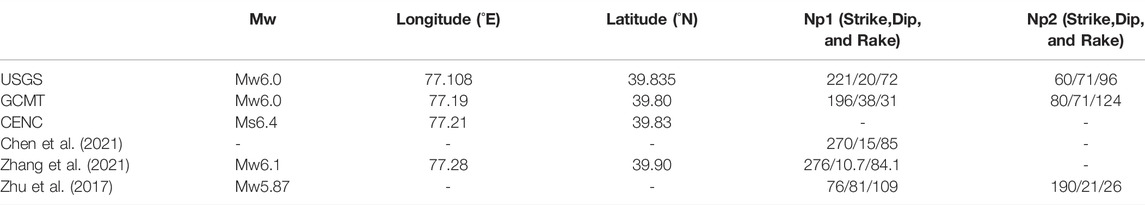
TABLE 1. Focal mechanism solutions of the Jiashi earthquake.

2 Regional Geological Background

The 2020 Jiashi Mw6.0 earthquake is another strong earthquake with a magnitude greater than Mw 6.0, which has occurred in the Jiashi earthquake swarm since 2003. A strong Jiashi earthquake swarm occurred in the northern margin of the Tarim Basin on the northeastern side of the Pamir Plateau, adjacent to the Tianshan arc nappe structural belt to the north (Figure 1). The Pamir Plateau is one of the regions with the strongest continental plate dynamics, while the Tianshan Mountains are typical intercontinental collision orogenic belts in the world (Lai et al., 2002). The epicenter was located in the South Tianshan foreland fold-thrust belt, with the Tianshan fold belt in the north, the West Kunlun-Pamir Plateau in the southwest, and the rigid Tarim Basin in the east and south. The Pamir Plateau is the deepest part of the Indian Plate and is wedged into the Eurasian continent. The Tianshan Mountains also experienced strong compression, uplift, folding, and thrust southward, forming a typical Cenozoic orogenic belt in the continental interior (Qiao and Guo, 2007; Zhang, 2003). The relative movement between the South Tianshan Mountains and Tarim Basin resulted in a large stress difference on the tectonic boundary, making the area more seismically active. In the past 20 years, most of the intense activities occurring in the southwestern Tianshan Mountains have been concentrated on the Kepingtage thrust fault (Tu. et al., 2008; Xu et al., 2006). The earthquake occurred in the western segment of the Kepingtage fault zone at the southern foot of the Tianshan Mountains. The Kepingtage Fault is located on the northwestern margin of the Tarim Basin, where there are several rows of arc-shaped thrusting rock ridges extending from EW to NE, forming an arc-shaped structural belt protruding to the southeast (Fang et al., 2009). The Kepingtage Fault is approximately 220 km long and is divided into two segments, east and west, by the SN-trending Piqiang fault zone. The Kepingtage Fault has strong seismic activity, causing the alluvial fan to rupture and form several faults and steep ridges at the foot of the Kepingtag Mountain. This makes the epicenter area present a complex topography with a relative height difference of several kilometers (Guo et al., 2021). Therefore, the tectonic conditions in this area are complex, and the tectonic activities are strong. Research on the mechanism of this earthquake is of great significance for an in-depth understanding of regional fault activity and earthquake prediction.

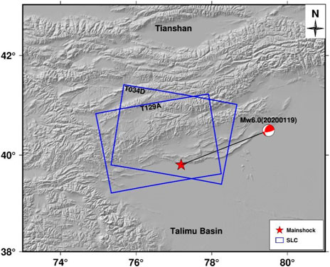
FIGURE 1. Geological overview of the study area.

3 Data and Processing

Sentinel-1A images were used to obtain the co-seismic deformation fields. Two images closest to the earthquake were selected to reduce the impact of post-earthquake deformation and decoherence noise on the co-seismic deformation field as much as possible. The pre-earthquake image in the ascending orbit was obtained on 16 January 2020, and the post-earthquake image was obtained on 28 January 2020. The pre-earthquake image in descending orbit was acquired on 10 January 2020, and the post-earthquake image was acquired on 22 January 2020. The related parameters are listed in Table 2. The perpendicular baselines of the interference pair are 9.4 m and -58.3 m, respectively (Table 2).

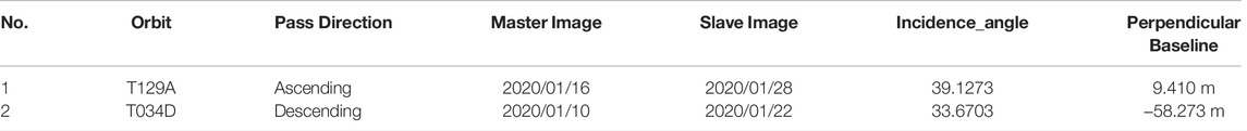
TABLE 2. Detailed parameters of the co-seismic interference pair.

Datasets were processed using the GAMMA software, which supports the whole process of SAR data processing (Werner et al., 2001). Differential interferometry (D-InSAR) was used to obtain the co-seismic deformation field (Massonnet et al., 1993; Shan, 2002), and the terrain phase was removed using the Shuttle Radar Topography Mission 30 m digital elevation model. We used precise orbital data to correct orbital deviation (https://s1qc.asf.alaska.edu/aux_poeorb/). The multi-look ratio in the range and azimuth was 8:2 to reduce noise in the interferogram. Because the phase in the original interferogram is wrapped, we adopted the minimum cost flow (MCF) method based on the Delaunay triangulation for phase unwrapping (Eineder et al., 1998; Werner and Wegmuller, 2002). Finally, we removed the terrain-related atmospheric delay error using the terrain correlation method.

Since the post-earthquake images from descending orbit have not been updated after 10 March 2020, they cannot meet the parameters required for long-term surface deformation monitoring. Therefore, we only collected Sentinel-1 SAR images from the ascending orbit to monitor post-earthquake deformation. A total of 32 images, covering the study area from 9 February 2020 to 23 March 2021, were processed using SBAS-InSAR. The SBAS-InSAR technology can generate a series of interferograms by setting temporal and spatial baseline thresholds. SBAS-InSAR technology not only ensures the quality of the interferograms but also increases the density of the coherent points. Differential processing and phase unwrapping are performed on high-quality interferograms, and finally, each subset is jointly solved by singular value decomposition (SVD) to obtain the time-series deformation (Berardino et al., 2002; Zhu, et al., 2017; Chen, et al., 2020). Interferograms were also multi-looked at a ratio of 8:2 in range and azimuth for post-earthquake deformation field monitoring. The spatial and vertical baselines were set at ±100 m and 80 days, respectively. The interference combinations are shown in Figure 2. Image registration was performed using amplitude-based image registration (Chen, et al., 2021). Gaussian filtering was applied to the interferograms to reduce noise and improve their coherence. Interferograms were unwrapped using the same method as that used for co-seismic deformation. A terrain-based correlation method was used to estimate and remove the atmospheric delay phase. Simultaneously, the trend error was estimated and eliminated based on a quadratic polynomial fitting model. Finally, interferograms with smaller atmospheric and unwrapping errors were selected and post-seismic deformation was obtained.

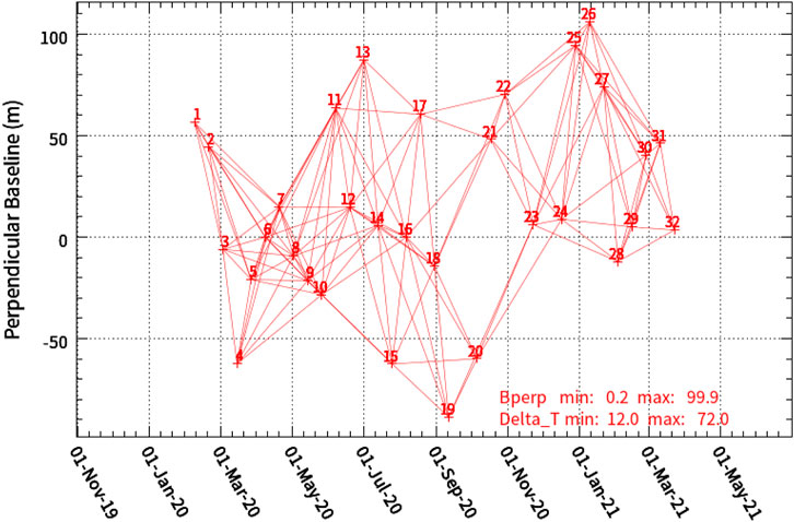
FIGURE 2. Interferometric combination of post-earthquake deformation field.

4 Co- and Post-seismic Deformation Analysis

4.1 Co-seismic Deformation Field

We obtained the co-seismic deformation field according to the above method (Figure 3). There are two thrust faults in this area (as shown in Figure 3): the Kepintag Fault and Ozgertawu Fault. Based on the monitoring results, the co-seismic deformation field was relatively integral and there was no sign of decoherence. This means that the fault did not rupture at the surface. The two deformation fields have the same situation, which is more consistent with others (Li, et al., 2021; Wen,et al., 2020; Wen-ting et al., 2020). The maximum uplift deformation in the line of sight (LOS) from the ascending images was 55 mm, and the maximum subsidence was 45 mm. The descending co-seismic deformation field showed that the maximum uplift and subsidence were 62 and 28 mm (Figure 2), respectively.

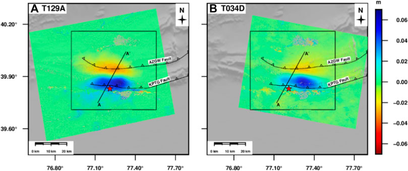
FIGURE 3. Co-seismic displacement field of Jiashi earthquake. (A) is from ascending interferogram (T129A); (B) is from descending interferogram (T034D).

We extracted a profile for the co-seismic deformation, and the results are shown in Figure 4A. We observed that the deformation trends along the profile were similar. There was a slight difference in magnitude. We adopted an internal coincidence accuracy evaluation method to verify the accuracy of the results. First, we selected the public area of the deformation field and converted the deformation in the LOS to vertical deformation according to the incidence of each pixel. Then, the results from the descending images in the vertical direction subtracted those from the ascending images, and statistical analysis was performed on the difference. The results are shown in Figure 4B. The difference conforms to a normal distribution, and the standard deviation is 11 mm.

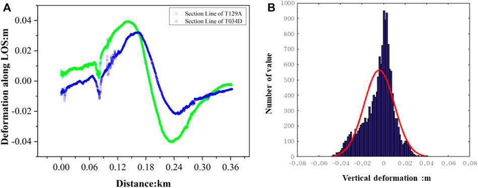
FIGURE 4. Co-seismic displacement profile of AA′ from T129A and T034D, and residual distribution of the co-seismic deformation field.

4.2 Post-earthquake Deformation Field

The period of an earthquake can be divided into three stages: interseismic, co-seismic, and post-seismic (Salvi et al., 2012). Interseismic refers to the relative motion of plates between two earthquakes. This is the process of accumulating energy when the fault is in a locked state. If the energy accumulation of the faults reaches a maximum, the fault reaches the critical rupture condition. At this time, an earthquake occurs and the accumulated energy is gradually released. Post-earthquake deformation is the response and adjustment of the crust and upper mantle to change and can directly reflect the rheological properties of the lithosphere. The temporal and spatial distribution of post-earthquake data varies greatly, and the time scale can range from a few days to a few months to hundreds of years (Bürgmann et al., 2001; Gourmelen and Amelung, 2005). Its spatial scale can span a few kilometers near a seismogenic fault (Jónsson et al., 2003) or across a global scale (Casarotti et al., 2001). Three models are usually used to describe post-earthquake deformation: afterslip (Harrington and Brodsky, 2006), the coupling effect between the lower crust and the upper mantle with viscoelastic relaxation properties (Pollitz et al., 2000), and the pore rebound effect of the crustal porous medium (Peltzer et al., 1996). After an earthquake, all three deformation mechanisms may exist and function in different spaces and times. The afterslip occurs because after the earthquake, the fault continues to slide in the direction of co-seismic due to inertia; afterslip plays a role in a short time after the earthquake. Poroelastic rebound is the same as afterslip, mainly occurring in the upper crust, and the deformation trend is opposite to that of co-seismic (Pollitz et al., 2000; Jónsson et al., 2003). The viscoelastic relaxation effect was caused by the stress change between the lower mantle and the upper crust. The viscoelastic relaxation effect plays a role for a long time after an earthquake, and the effect in the far-field is more substantial (Pollitz et al., 2000). Therefore, we believe that the short-term viscoelastic relaxation effect was not the post-seismic deformation mechanism of this earthquake.

After an earthquake, the energy accumulated is often released slowly during the main shock and post-seismic events, squeezing the surrounding faults, and deforming the surrounding fractures, resulting in aftershocks. To analyze the influence of the post-earthquake on the surrounding faults, we used the SBAS-InSAR to obtain the deformation field after the earthquake, since the epicenter of the earthquake was relatively close to the Kepintag and Ozgwu faults (Figure 5). The time span of post-earthquake images is from 9 February 2020, to 23 March 2021. During the 447 days, the results showed that the overall uplift was dominant between the Kepingtage fault and the Ozgwu fault, with a maximum uplift of 8 mm (Figure 5). However, south of the Kepingtage fault is in a subsidence state, indicating that the blocks between the two faults are in a state of compression. Simultaneously, post-earthquake deformation mainly occurs on the fault, which belongs to the stress change caused by co-seismic rupture. The post-seismic deformation trend was the same as that of the co-seismic deformation, so the poroelastic rebound effect was excluded. Therefore, we initially believe that the post-earthquake deformation mechanism was an afterslip. In addition, aftershocks were distributed in the area with a larger deformation (Figure 5). We selected a point (square in Figure 5) in the region with significant deformation characteristics to extract the post-earthquake deformation time series (Figure 6). We used a post-earthquake afterslip model function to fit the post-earthquake deformation time series at this point (Barnhart et al., 2018)

where y is the accumulated deformation in the LOS(m), t is the time interval from the mainshock after the earthquake, and a represents the coefficient of the logarithmic function.

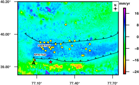
FIGURE 5. Post-earthquake deformation rate. Yellow circles: aftershock, red star: epicenter, rectangle: selected point, KPTG and AZGW: two faults.

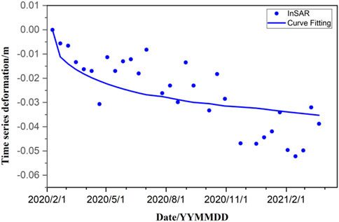
FIGURE 6. Post-earthquake deformation time series and a fitting result at point A.

The results show that when a = -0.01264 and $\text{t}$ = 240 days after the main shock, the fitting results agree with the post-earthquake deformation time series results. The post-earthquake deformation trend is consistent with co-seismic deformation. Based on the extracted post-earthquake deformation time series, we believe that the post-earthquake deformation mechanism of the Jiashi earthquake was an afterslip.

5 Inversion and Analysis of Fault

The inversion of co-seismic deformation is one of the important means to improve the understanding of seismogenic structures and to evaluate regional earthquake disasters. In this paper, the Okada elastic dislocation model is used to study the co-seismic deformation. The inversion is divided into two parts. First, we assumed that the slip was uniform, and the Geodetic Bayesian Inversion Software (GBIS) was used to search for the source parameters. The fault is further divided into patches after the geometric parameters of the fault are obtained and the slip of each patch is calculated.

5.1 Co-seismic Uniform Slip Inversion

The inversion for this earthquake was implemented using the Okada elastic dislocation model in the open-source software GBIS (Bagnardi and Hooper, et al., 2018). It is necessary to downsample the InSAR data before inversion to improve efficiency. We adopted the quadtree sampling method, which can retain more points in the region with large deformation and retain fewer points in the region with smaller deformation. Co-seismic deformation inversion was then performed by setting the source parameters of the fault. The parameters included length, width, depth, strike angle, dip angle, strike-slip, and dip-slip. The Okada elastic dislocation model is equivalent to treating a seismogenic fault as a rectangle embedded in a uniform elastic half-space model. In the inversion, the parameter was set to a length of 1–80 km, width of 3–80 km, depth of 5–80 km, strike angle of 90°–360°, and dip angle of 0–90°, with the strike-slip and dip-slip being -2 and 2 m, respectively. The Monte Carlo search method was used to search, and the best fitting value of each parameter of the fault was obtained, including the optimal and average values. The inversion results are presented in Table 3. Figure 7 shows InSAR observations, models, and residuals. It can be seen that the model results reflect the InSAR observations well, and there are residuals at some epicenter points. The inversion results showed that the dip-slip was considerably larger than the strike-slip, and that the seismogenic fault was dominated by a dip-slip. The depth of the epicenter is 7.2 km, which is greater than the width 4.65 km of the fault, indicating that the seismogenic fault does not appear exposed to the surface.

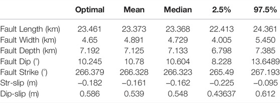
TABLE 3. Fault parameters for uniform slip inversion.

FIGURE 7. Comparison of non-linear inversion results. (A), (B), (C) are observation ,model,residual from T064A respectively (D), (E), (F) are observation ,model, residual from T034D respectively.

5.2 Co-seismic Slip Distribution Inversion

The co-seismic deformation field can only grasp the destructiveness, damage range, and magnitude of the earthquake but cannot determine the geological structure of the earth’s internal faults and the direction information of the seismogenic faults. Therefore, to analyze the geological structure of this earthquake, we used the SDM inversion program (Wang, et al., 2013a; Wang, et al., 2013b) to calculate the slip distribution of faults using the Okada elastic half-space dislocation model (Xu et al., 2010; Motagh et al., 2015). During the inversion, a co-seismic deformation field was used as the constraint, and an initial fault geometric model was established according to the GBIS inversion. Simultaneously, the fault was appropriately extended along the strike and dip, and the seismogenic fault was set to 60 km × 40 km. We divided the fault into 2 × 2 km patches along the strike and dip, with a total of 600 patches. The smoothing factor was determined by weighing the compromise curve between the roughness and the residual. Finally, a smoothing factor of 0.05 was selected as the optimal result (Figure 8). The distributed slip inversion is shown in Figure 9. The fitting result between the observation and the model was 96.2%, indicating our optimal model can fit the fault geometry reasonably well. Compared with others, the rectangular dislocation model can inverse this co-seismic deformation well. The residuals of the distributed slip inversion were considerably reduced compared with the uniform slip distribution inversion. Figure 9 indicates that the ruptures are concentrated 22–46 km along the strike and 10–18 km along the dip. The average slip angle was −176.29°, the average slip was 0.04 m, and the magnitude was Mw6.1, indicating the co-seismic fault to be a reverse fault with a small strike-slip motion (Figure 10). According the focal mechanism solution from Table 1, this earthquake belongs to thrust type, indicating that our result is consistent with the USGS and GCMT. As shown in Figure 10, the epicenter of the Jiashi earthquake was located on the Kepingtag fault. We believe that this was a dip-slip earthquake that occurred on the Kepingtag nappe belt.

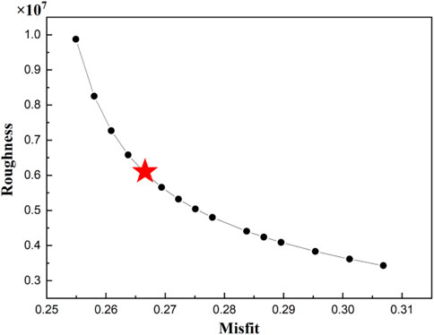
FIGURE 8. Roughness and fitting residual curve.

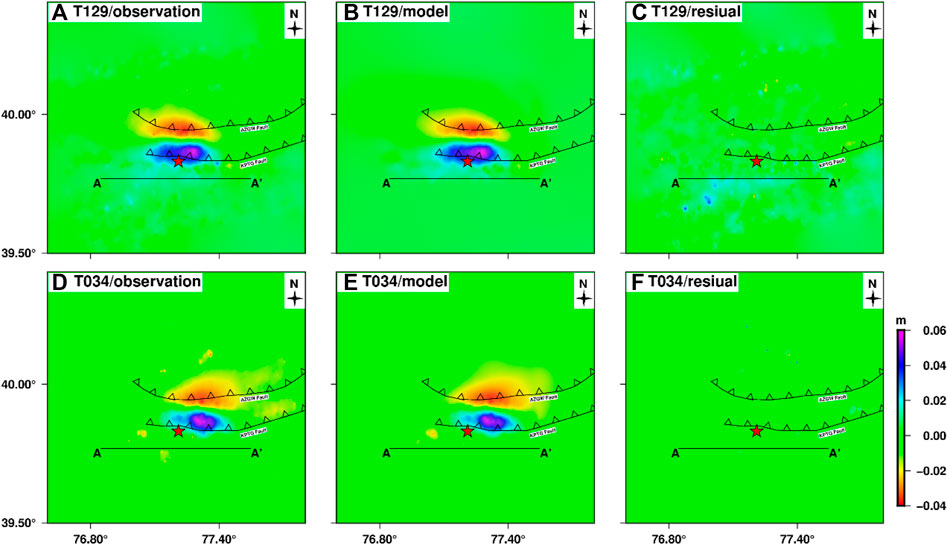
FIGURE 9. Distributed slip inversion results. (A), (B), and (C) are observation, model, and residual, respectively, of T129A; (D), (E), and (F) are observation, model, residual, respectively, of T034D.

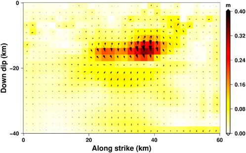
FIGURE 10. Two-dimensional slip distribution. The arrow indicates the movement direction of the block.

5.3 Post-earthquake Deformation Inversion

Figure 4 shows that the post-earthquake deformation and aftershocks are mainly concentrated between the Keping and Ozgwu faults and are located near the seismogenic fault. We used the SDM method to invert the accumulated deformation within 447 days after the earthquake to further analyze the post-earthquake deformation mechanism. According to the post-earthquake deformation, we set the fault length to 60 km and width to 48 km, to invert the post-earthquake slip distribution. The InSAR observations, model, and residuals are shown in Figures 11A,B,C, respectively. From the inversion, the simulation effect of the main deformation region after the earthquake was good and the residual was relatively small. Some minor deformations have not been simulated south of the Ozgwu Fault. Larger residuals were mainly distributed in the northwest corner (Figure 11), which may be related to the viscoelastic relaxation effect or tectonic movement changes. Figure 12 shows the post-earthquake two-dimensional slip distribution. Several slip patches were found in the shallow fault layer. The first slip is located to the west of the Keping fault, approximately 14 km from the epicenter, 0–12 km along the strike, and 0–9 km along the dip, and the slip is 0.06 m. The second slip was located to the north of the epicenter, far from the epicenter, 15–24 km along the strike, and 36–45 km along the dip, and the slip reaches 0.05 m. These phenomena indicate that the post-earthquake geological tectonic activity in this area was only more active in these two places, and the magnitude was also small. Regional tectonic activity gradually stabilized after the earthquake, and further earthquakes were less likely.

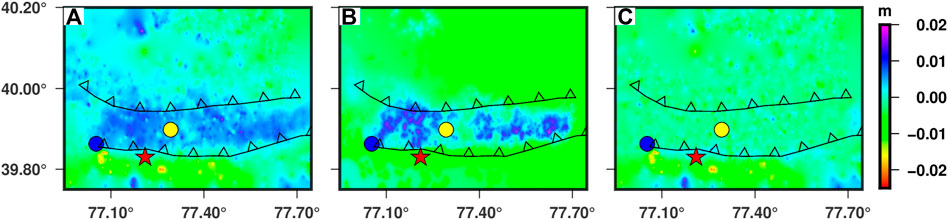
FIGURE 11. Post-earthquake deformation inversion results. (A), (B), and (C) are observation, model, and residual, respectively. Yellow circles represent the largest co-seismic slip, and blue circles represent the largest post-earthquake slip.

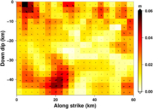
FIGURE 12. Two-dimensional slip distribution results of faults after earthquake.

Comparing the results of the co-seismic and post-earthquake slip distributions, the maximum slip of the co-seismic is 0.32 m and post-earthquake depth is 3.88 km. The maximum slip of post-earthquake is 0.06 m and the depth is 0.31 km. The maximum slip of co-seismic and the post-earthquake occurred on the same fault plane and were separated by 20 km. The post-earthquake deformation mechanism exhibits thrust and strike-slip, while co-seismic belongs to thrust. Similar mechanisms exist, but the co-seismic and post-seismic maximum slip patches are located at different locations on the same fault plane, suggesting that the post-seismic motion is likely driven by stress concentrations at the co-seismic patch edges (Amiri et al., 2020).

6 Discussion

6.1 Earthquake Analysis

Presently, the greater the intensity and frequency of intermediate seismic activity in the western Himalayan tectonic structure, the more intense the strong earthquake activity in the Tianshan seismic belt. The active periods of several strong earthquakes in the history of the Tianshan area show migration from west to east (Zhang and Shao, 2014). This indicates that there is a dynamic relationship between the strong earthquake of the western Himalayan tectonic structure and the strong activity of the Tianshan seismic belt in Xinjiang, China, i.e., the West Himalayan tectonic knot has a triggering effect on the seismic activity of the Tianshan seismic belt. The earthquake occurred in the South Tianshan foreland fold-thrust belt, which is located northeast of the Pamir Plateau. The Pamir Plateau structure is mainly affected by the combined action of the northward subduction of the Indian plate and the southward subduction of the Tianshan Mountains (Sippl et al., 2013), indicating that the Tianshan Block is thrust over the Tarim Basin. In such tectonic environments, moderate and strong earthquakes occur frequently in the Jiashi area. The Jiashi Mw6.0 earthquake occurred in an area with substantial thrusting movement and was an inevitable rupture event under a prominent tectonic background with a typical thrusting movement.

6.2 Coulomb Stress

The rupture of a co-seismic fault causes the redistribution of the surrounding stress. Based on Coulomb3.3 (Lin and Stein, 2004; Toda et al., 2005), we assumed that the shear modulus was 3.2 × 10⁴ MPa; moreover, the friction coefficient was set to 0.4, and the Poisson’s ratio was 0.25. Combined with the co-seismic slip distribution, we calculated Coulomb stress changes (Figure 13A). Simultaneously, taking the thrust fault as the receiver faults, the Coulomb stress was calculated at depths of 5 and 10 km (Figures 13B,C). If the Coulomb stress is positive, it is called the stress-loading area, and the corresponding risk increases. Conversely, if the Coulomb rupture stress is negative, fault rupture will be suppressed. The negative area is called the “stress shadow area,” wherein the possibility of triggering an earthquake will be weakened (Yongge et al., 2002). However, this is an ideal scenario. The Coulomb stress distribution is more complicated and is generally affected by the fault geometry, crust, Green’s function, and errors in observational data. Therefore, the calculation results of the Coulomb stress should be analyzed in detail. The result indicated that the co-seismic coulomb stress distribution was negative near the epicenter, suggesting that it was in a state of stress release. As the depth of projection increases, the stress range decreases gradually. The Coulomb stress at a depth of 5 km was in a state of stress loading near the epicenter, and the positive value of stress loading was around the Kepintag fault (Figure 13B). The depth was 10 km, and the stress loading was relieved. The Coulomb stress distribution is in good agreement with the shallow fault deformation mechanism, which may be related to various factors such as the actual fault geometry and formation properties.

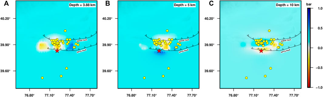
FIGURE 13. Coulomb stress distribution at different depths. Red star: epicenter, yellow circle: the aftershock. Aftershock data was obtained from CENC.

7 Conclusion

We used Sentinel-1A images and D-InSAR to obtain the co-seismic deformation field of the 2021 Jiashi earthquake. The monitoring results show that the maximum uplift caused by the earthquake is 62 mm, located south of the epicenter, with a maximum subsidence of -45 mm, located north of the epicenter. The inversion of the Okada elastic uniform half-space model shows that the earthquake was induced by a length of 23.5 km, a width of 4.7 km, and a depth of 7.2 km. At the same time, the dip-slip component is larger than the strike-slip component, indicating that the seismic fault plane is dominated by dip-slip. The co-seismic slip distribution showed that the magnitude was Mw6.1, the main slip was concentrated at 22–46 km along the strike and 10–18 km along the dip, and the average slip angle was -176.29°. The regional fault is thrust with a small strike-slip component, which is consistent with the focal mechanism solution results given by the USGS, GCMT, and other institutions. Post-earthquake deformation monitoring based on SBAS InSAR technology showed that the post-earthquake deformation rate was 25 mm/yr within 447 days. The nature of the movement between them is uplifting deformation, and the post-earthquake deformation mechanism is afterslip.

Data Availability Statement

The original contributions presented in the study are included in the article/Supplementary Material, further inquiries can be directed to the corresponding author.

Author Contributions

SZ and CY conceived and designed the experiments; TW performed the experiments and drafted the manuscript. HH processed Sentinel-1A images. YW provided some suggestions of writing. CZ contributed to the InSAR and earthquake analysis.

Funding

This research was financed by the National Natural Science Foundation of China (NSFC) (No. 42174032), the Fundamental Research Funds for the Central Universities (CHD300102262206).

Conflict of Interest

The authors declare that the research was conducted in the absence of any commercial or financial relationships that could be construed as a potential conflict of interest.

Publisher’s Note

All claims expressed in this article are solely those of the authors and do not necessarily represent those of their affiliated organizations, or those of the publisher, the editors and the reviewers. Any product that may be evaluated in this article, or claim that may be made by its manufacturer, is not guaranteed or endorsed by the publisher.

Acknowledgments

We acknowledge the European Space Agency (ESA) for freely making available the Sentinel-1A data. Maps were prepared using the Generic Mapping Tools (GMT), Matlab and Origin software.

References

Amiri, M., Mousavi, Z., Atzori, S., Khorrami, F., Aflaki, M., Tolomei, C., et al. (2020). Studying Postseismic Deformation of the 2010–2011 Rigan Earthquake Sequence in SW Iran Using Geodetic Data. Tectonophysics 795, 228630. doi:10.1016/j.tecto.2020.228630
Bagnardi, M., and Hooper, A. (2018). Inversion of Surface Deformation Data for Rapid Estimates of Source Parameters and Uncertainties: A Bayesian Approach. Geochem. Geophys. Geosyst. 19, 2194–2211. doi:10.1029/2018gc007585
Barnhart, W. D., Brengman, C. M. J., Li, S., and Peterson, K. E. (2018). Ramp-flat Basement Structures of the Zagros Mountains Inferred from Co-seismic Slip and Afterslip of the 2017 Mw7.3 Darbandikhan, Iran/Iraq Earthquake. Earth Planet. Sci. Lett. 496, 96–107. doi:10.1016/j.epsl.2018.05.036
Berardino, P., Fornaro, G., Lanari, R., and Sansosti, E. (2002). A New Algorithm for Surface Deformation Monitoring Based on Small Baseline Differential SAR Interferograms. IEEE Trans. Geosci. Remote Sens. 40, 2375–2383. doi:10.1109/tgrs.2002.803792
Bürgmann, R., Kogan, M. G., Levin, V. E., Scholz, C. H., King, R. W., and Steblov, G. M. (2001). Rapid Aseismic Moment Release Following the 5 December, 1997 Kronotsky, Kamchatka, Earthquake. Geophys. Res. Lett. 28, 1331–1334. doi:10.1029/2000GL012350
Casarotti, E., Piersanti, A., Lucente, F. P., and Boschi, E. (2001). Global Postseismic Stress Diffusion and Fault Interaction at Long Distances. Earth Planet. Sci. Lett. 191, 75–84. doi:10.1016/s0012-821x(01)00404-6
Chen, B., Li, Z., Yu, C., Fairbairn, D., Kang, J., Hu, J., et al. (2020). Three-dimensional Time-Varying Large Surface Displacements in Coal Exploiting Areas Revealed through Integration of SAR Pixel Offset Measurements and Mining Subsidence Model. Remote Sens. Environ. 240, 111663. doi:10.1016/j.rse.2020.111663
Chen, B., Mei, H., Li, Z., Wang, Z., Yu, Y., and Yu, H. (2021). Retrieving Three-Dimensional Large Surface Displacements in Coal Mining Areas by Combining SAR Pixel Offset Measurements with an Improved Mining Subsidence Model. Remote Sens. 13 (13), 2541. doi:10.3390/rs13132541
Eineder, M., Hubig, M., and Milcke, B. (1998). “Unwrapping Large Interferograms Using the Minimum Cost Flow Algorithm,” in Proceedings of the IEEE International Geoscience & Remote Sensing Symposium, Seattle, WA, USA, 6-10 July 1998. doi:10.1109/igarss.1998.702806
Fang, M. L., Wang, S. H., Han, X. Q., and Zhao, S. Q. (2009). Trend Connection and Genetic Analysis of Cenozoic Nappe Rock Sheets in Keping. Xinjiang. China Geol. 36, 322–333. (in Chinese).
Gourmelen, N., and Amelung, F. (2005). Postseismic Mantle Relaxation in the Central Nevada Seismic Belt. Science 310, 1473–1476. doi:10.1126/science.1119798
Guo, Z., Gao, X., and Lu, Z. (2021). Relocation and Focal Mechanism of the Jiashi M6.4 Earthquake on January 19, 2020, in Xinjiang [J]. Earthq. Geol. 43, 345–356. (in Chinese).
Harrington, R. M., and Brodsky, E. E. (2006). The Absence of Remotely Triggered Seismicity in Japan. Bull. Seismol. Soc. Am. 96, 871–878. doi:10.1785/0120050076
Jónsson, S., Segall, P., Pedersen, R., and Björnsson, G. (2003). Post-Earthquake Ground Movements Correlated to Pore-Pressure Transients. Nature 424, 179–183. doi:10.1038/nature01776
Lai, Y. G., Liu, Q. Y., Chen, J. H., Guo, S., and Li, S. C. (2002). Shear Wave Splitting and Stress Field Characteristics in the Strong Earthquake Cluster in Jiashi, Xinjiang. Chin. J. Geophys. 01, 83.
Li, C. L., Zhang, G. H., Shan, X. J., Qu, C. Y., Gong, W. Y., Jia, R., et al. (2021). Advances in Geophysics InSAR Coseismic Deform. Field Fault SLIP Distrib, 6.4 Earthquake in Jiashi County, Xinjiang on January 19, 2020. Inversion Ms 36, 481–488. (in Chinese).
Lin, J., and Stein, R. S. (2004). Stress Triggering in Thrust and Subduction Earthquakes and Stress Interaction between the Southern San Andreas and Nearby Thrust and Strike-Slip Faults. J. Geophys. Res. 109, B02303. doi:10.1029/2003jb002607
Massonnet, D., Rossi, M., Carmona, C., Adragna, F., Peltzer, G., Feigl, K., et al. (1993). The Displacement Field of the Landers Earthquake Mapped by Radar Interferometry. Nature 364, 138–142. doi:10.1038/364138a0
Motagh, M., Bahroudi, A., Haghighi, M. H., Samsonov, S., Fielding, E., and Wetzel, H.-U. (2015). The 18 August 2014 Mw 6.2 Mormori, Iran, Earthquake: A Thin-Skinned Faulting in the Zagros Mountain Inferred from InSAR Measurements. Seismol. Res. Lett. 86, 775–782. doi:10.1785/0220140222
Peizhen, Z. (2003). Late Cenozoic Tectonic Deformation of Tianshan and its Foreland Basins. Sci. Bull. 48, 2499–2500. (in Chinese). doi:10.1007/BF02900310
Peltzer, G., Rosen, P., Rogez, F., and Hudnut, K. (1996). Postseismic Rebound in Fault Step-Overs Caused by Pore Fluid Flow. Science 273, 1202–1204. doi:10.1126/science.273.5279.1202
Pollitz, F. F., Peltzer, G., and Bürgmann, R. (2000). Mobility of Continental Mantle: Evidence from Postseismic Geodetic Observations Following the 1992 Landers Earthquake. J. Geophys. Res. 105, 8035–8054. doi:10.1029/1999jb900380
Qiao, X. J., and Guo, L. M. (2007). SAR Observational Study of Strong Earthquake Cluster in Jiashi, Xinjiang. Geod. Geodyn. 27, 7–13. (in Chinese).
Ren, J., Yalikun, A., Li, Z. Q., Wen, H. P., and Li, X. L. (2020). Accuracy Analysis of Rapid Damage Assessment for Ms6.4 Earthquake in Jiashi, Xinjiang, on January 19, 2020. Earthq. Disaster Prev. Technol. 15, 349–358. (in Chinese). doi:10.11899/zzfy20200212
Salvi, S., Stramondo, S., Funning, G. J., Ferretti, A., Sarti, F., and Mouratidis, A. (2012). The Sentinel-1 Mission for the Improvement of the Scientific Understanding and the Operational Monitoring of the Seismic Cycle. Remote Sens. Environ. 120, 164–174. doi:10.1016/j.rse.2011.09.029
Shan, X. J., Ma, J., Wang, C. L., Liu, J. H., Song, X. X., and Zhang, G. F. (2002). Extraction of the Focal Fault Parameters of the Mani Earthquake by Using the Surface Deformation Field Obtained by the Spaceborne D-INSAR Technology. Sci. China D. 32, 837–844. (in Chinese).
Sippl, C., Schurr, B., Yuan, X., Mechie, J., Schneider, F. M., Gadoev, M., et al. (2013). Geometry of the Pamir‐Hindu Kush Intermediate‐depth Earthquake Zone from Local Seismic Data. JGR Solid Earth 118, 1438–1457. doi:10.1002/jgrb.50128
Toda, S., Stein, R. S., and Richards Dinger, K. (2005). Forecasting the Evolution of Seismicity in Southern California: Animations Built on Earthquake Stress Transfer. J. Geophys. Res. 110. B05S16. doi:10.1029/2004JB003415
Tu, H. W., Wan, X. H., Gao, G., Luo, G. F., Hu, Y. J., and Ma, Z. (2008). Preliminary Study on Fault Properties and Stress Field Changes during the Jiashi Earthquake in Xinjiang from 1977 to 2006. Prog. Geophys. 23, 1038–1044. (in Chinese).
Wan, Y. G., Wu, Z. L., Zhou, G. W., Huang, J., and Qin, L. X. (2002). Research on Earthquake Stress Triggering. Acta Seismol. Sin. 2002 (5), 533–551.
Wang, R. J., Diao, F., and Hoechner, A. (2013a). SDM-A Geodetic Inversion Code Incorporating with Layered Crust Structure and Curved Fault Geometry. EGU General Assem., 2013–2411.
Wang, R., Parolai, S., Ge, M., Jin, M., Walter, T. R., and Zschau, J. (2013b). The 2011 Mw 9.0 Tohoku Earthquake: Comparison of GPS and Strong-Motion Data. Bull. Seismol. Soc. Am. 103, 1336–1347. doi:10.1785/0120110264
Wen, S. Y., Li, C. L., Li, J., et al. (2020). Inland Earthquakes. Preliminary Discussion on. InSAR Coseismic Deform. Field Charact. Seismogenic Struct. Ms6.4 Jiashi Earthq. Xinjiang January 19 34, 1–9. (in Chinese). doi:10.16256/j.issn.1001-8956.2020.01.001
Werner, C., Wegmuller, U., and Strozzi, T. (2002). “Processing Strategies for Phase Unwrapping for INSAR Applications,” in Proceedings EUSAR, Cologne, June 4–6, 2002.
Werner, C., Wegmüller, U., Strozzi, T., and Wisemann, A. (2001). “Gamma SAR and Interferometric Processing Software,” in Proceedings of the ERS ENVISAT Symposium, Gothenburg, Sweden, 16-20 October 2001.
Wessel, P., Luis, J. F., Uieda, L., Scharroo, R., Wobbe, F., Smith, W. H. F., et al. (2019). The Generic Mapping Tools Version 6. Geochem. Geophys. Geosyst. 20, 5556–5564. version 6. 20. doi:10.1029/2019gc008515
Xu, C., Liu, Y., Wen, Y., and Wang, R. (2010). Coseismic Slip Distribution of the 2008 Mw 7.9 Wenchuan Earthquake from Joint Inversion of GPS and InSAR Data. Bull. Seismol. Soc. Am. 100, 2736–2749. doi:10.1785/0120090253
Xu, X. W., Zhang, X. K., Ran, Y. K., Cui, X. F., Ma, W. T., Sheng, J., et al. (2006). A Preliminary Study on the Seismogenic Structure of the Bachu-Jishi Earthquake (Ms6.8) in the Southern Tianshan Area. Earthq. Geol. 28, 161–178. (in Chinese).
Zhang, L. P., and Shao, Z. G. (2014). Analysis on Correlativity between Large Earthquakes in the Hindu Kush-Pamir and Tienshan Seismic Zone. Earthq. Res. China. 28, 177–187.
Zhang, W. T., Ji, L. Y., Zhu, L. Y., et al. (2021). A Typical Thrust Rupture Event Occurring in the Foreland Basin of the Southern Tianshan: The 2020 Xinjiang Jiashi MS 6. 4 Earthquake. Seismol. Geol. 43, 394–409. (in Chinese).
Keywords: jiashi earthquake, co-seismic deformation, post-earthquake deformation, slip distribution, coulomb stress
Citation: Wang T, Zhu SN, Yang CS, Wei YJ, Zhao CY and Hou HC (2022) Co- and Post-seismic Deformation Mechanisms of the 2020 Mw6.0 Jiashi Earthquake in Xinjiang (China), Revealed by Sentinel-1 InSAR Observations. Front. Environ. Sci. 10:933200. doi: 10.3389/fenvs.2022.933200
Received: 30 April 2022; Accepted: 14 June 2022;
Published: 22 July 2022.
Edited by:
Yu Chen, China University of Mining and Technology, ChinaReviewed by:
Hong'An Wu, Chinese Academy of Surveying and Mapping, ChinaZhiwei Zhou, Innovation Academy for Precision Measurement Science and Technology, (CAS), China
Jinwoo Kim, Southern Methodist University, United States
Copyright © 2022 Wang, Zhu, Yang, Wei, Zhao and Hou. This is an open-access article distributed under the terms of the Creative Commons Attribution License (CC BY). The use, distribution or reproduction in other forums is permitted, provided the original author(s) and the copyright owner(s) are credited and that the original publication in this journal is cited, in accordance with accepted academic practice. No use, distribution or reproduction is permitted which does not comply with these terms.
*Correspondence: S. N. Zhu, jcyzhusainan@mail.cgs.gov.cn