Upscaling Methane Flux From Plot Level to Eddy Covariance Tower Domains in Five Alaskan Tundra Ecosystems
 Yihui Wang1
  Fengming Yuan2 Kyle A. Arndt3 Jianzhao Liu4
  Liyuan He1
  Yunjiang Zuo4 Donatella Zona1
  David A. Lipson1 Walter C. Oechel1
  Daniel M. Ricciuto2
  Stan D. Wullschleger2
  Peter E. Thornton2
  Xiaofeng Xu1*
- 1Department of Biology, San Diego State University, San Diego, CA, United States
- 2Environmental Sciences Division, Oak Ridge National Laboratory, Oak Ridge, TN, United States
- 3Earth Systems Research Center, Institute for the Study of Earth, Oceans, and Space, University of New Hampshire, Durham, NH, United States
- 4Key Laboratory of Wetland Ecology and Environment, Northeast Institute of Geography and Agroecology, Chinese Academy of Sciences, Beijing, China
Spatial heterogeneity in methane (CH4) flux requires a reliable upscaling approach to reach accurate regional CH4 budgets in the Arctic tundra. In this study, we combined the CLM-Microbe model with three footprint algorithms to scale up CH4 flux from a plot level to eddy covariance (EC) tower domains (200 m × 200 m) in the Alaska North Slope, for three sites in Utqiaġvik (US-Beo, US-Bes, and US-Brw), one in Atqasuk (US-Atq) and one in Ivotuk (US-Ivo), for a period of 2013–2015. Three footprint algorithms were the homogenous footprint (HF) that assumes even contribution of all grid cells, the gradient footprint (GF) that assumes gradually declining contribution from center grid cells to edges, and the dynamic footprint (DF) that considers the impacts of wind and heterogeneity of land surface. Simulated annual CH4 flux was highly consistent with the EC measurements at US-Beo and US-Bes. In contrast, flux was overestimated at US-Brw, US-Atq, and US-Ivo due to the higher simulated CH4 flux in early growing seasons. The simulated monthly CH4 flux was consistent with EC measurements but with different accuracies among footprint algorithms. At US-Bes in September 2013, RMSE and NNSE were 0.002 μmol m−2 s−1 and 0.782 using the DF algorithm, but 0.007 μmol m−2 s−1 and 0.758 using HF and 0.007 μmol m−2 s−1 and 0.765 using GF, respectively. DF algorithm performed better than the HF and GF algorithms in capturing the temporal variation in daily CH4 flux each month, while the model accuracy was similar among the three algorithms due to flat landscapes. Temporal variations in CH4 flux during 2013–2015 were predominately explained by air temperature (67–74%), followed by precipitation (22–36%). Spatial heterogeneities in vegetation fraction and elevation dominated the spatial variations in CH4 flux for all five tower domains despite relatively weak differences in simulated CH4 flux among three footprint algorithms. The CLM-Microbe model can simulate CH4 flux at both plot and landscape scales at a high temporal resolution, which should be applied to other landscapes. Integrating land surface models with an appropriate algorithm provides a powerful tool for upscaling CH4 flux in terrestrial ecosystems.
1 Introduction
Northern Arctic tundra is characterized by polygonal patterns due to freeze-thaw cycles with large spatial heterogeneity in vegetation and soil water table (Budishchev et al., 2014; Petrescu et al., 2015; Lara et al., 2020). This heterogeneity leads to a large spatial variability of methane (CH4) flux (Xu et al., 2010; Budishchev et al., 2014), as the production, consumption, and transport processes of CH4 are primarily related to hydrology, vegetation, and microbial activities (Vaughn et al., 2016). Modeling and predicting the spatial variability of CH4 emissions at broader scales depend on the upscaling algorithms that consider heterogeneous landscapes (Davidson et al., 2016; Xu et al., 2016). At the plot scale (10–2–1 m2), closed chambers are commonly employed to measure CH4 flux for dominant topography and/or vegetation types (Fox et al., 2008; Davidson et al., 2016). Numerous empirical and mechanistic modeling studies have attempted to upscale these measurements to the landscape scale (104–105 m2) and evaluated them against eddy covariance (EC) flux (Baldocchi, 2008; Chen et al., 2012; Xu and Tian, 2012; Davidson et al., 2017). Yet, these estimates ignored the impact of the spatial variability of CH4 flux within the source area. Accurate regional estimations of CH4 flux require an upscaling approach that considers the mechanistic CH4 processes, including the key factors that control CH4 flux across time and space (Xu et al., 2016).
Factors affecting Arctic CH4 emission vary substantially across spatial scales (Mer and Roger, 2001; Serrano-Silva et al., 2014; Xu et al., 2016). The soil water table has been identified as a key factor determining the CH4 flux (Funk et al., 1994; Pirk et al., 2017). In addition, plant coverage and composition play an important role in CH4 emission by affecting CH4 transport pathway and providing substrate for methanogens (von Fischer et al., 2010; Bhullar et al., 2013; McEwing et al., 2015; Davidson et al., 2016). Greater vascular plant coverage and density were linked to higher CH4 emission (McEwing et al., 2015; Andresen et al., 2017), and vegetation types can explain a large proportion of the variation in CH4 flux in Arctic tundra (Sturtevant and Oechel, 2013; Davidson et al., 2016). This is because sedges and vascular wetland plants not only exist in waterlogged areas prime for CH4 production, but they also transport CH4 through their tissue straight to the atmosphere (Lai, 2009). Therefore, it is critically important to include vegetation characteristics within an EC footprint to improve the accuracy of CH4 estimation at the landscape scale. In most CH4 models (Xu et al., 2016), vegetation is represented as plant functional types (PFTs), and in each PFT group, plant species share similar responses to environmental factors (Langford et al., 2016). Therefore, it is critically important to integrate mechanistic models of CH4 cycling with high-resolution spatial datasets of vegetation coverage and environmental factors to improve the accuracy of estimations of CH4 flux at the landscape scale.
The process-based CLM-Microbe model has been tested in simulating plot-scale CH4 flux by validating with different polygonal characteristics’ (e.g. troughs, rims, and centers) flux at Utqiagvik, Alaska (Wang et al., 2019). In the previous study, we upscaled model-simulated flux from the plot to landscape scales and validated it with EC measurements using the area-weighted average approach (Wang et al., 2019). However, this approach can be rather inaccurate because the contribution of areas in upscaling might be different within the EC tower footprint, leading to a significant mismatch (Oechel et al., 1998; Fox et al., 2008). Accurate knowledge of footprints is of crucial importance for upscaling from plot-scale flux measurements to the landscape scale. Flux footprint algorithms generate the spatial extent and position of the probable source area for EC flux measurements by integrating effects of wind direction and speed, roughness at a specific time point, thereby they are widely used for understanding EC estimates and improving greenhouse gas budgets (Horst and Weil, 1992; Kormann and Meixner, 2001; Kljun et al., 2015; Heidbach et al., 2017). In our study, we combined the CLM-Microbe model with three footprint algorithms to better scale up to the landscape-scale CH4 flux. The CLM-Microbe model represents 17 PFTs for vegetation across the globe (Wang et al., 2019; He et al., 2021a; He et al., 2021b); adding Arctic- and boreal-specific PFTs in its vegetation modules makes it more appropriate to capture Arctic vegetation processes.
This study was designed to apply the CLM-Microbe model to simulate plot-scale CH4 flux with a fine spatial resolution for five study sites in the Alaskan Arctic tundra. By incorporating different footprint algorithms, we upscaled the simulated plot-scale flux to the EC domain and validated it with the EC measurements. In this study, we aim to 1) evaluate the accuracy of CH4 estimates simulated by the CLM-Microbe model with different footprint algorithms, 2) compare the homogenous footprint algorithm (HF), gradient footprint algorithm (GF), and dynamic footprint algorithm (DF) for assisting upscaling CH4 flux, and 3) investigate the primary controlling factors of CH4 emission at the landscape scale in the Arctic tundra ecosystems.
2 Methodology
2.1 Site Information and Experimental Data
2.1.1 Site Description
We performed our study at five sites in the northern Alaskan tundra (Figure 1), and detailed information on sites and measurements is available (Arndt et al., 2020; Arndt et al., 2019). Three of these sites are located in Utqiaġvik (formerly Barrow), including US-Beo (71.2810°N, 156.6124°W), US-Bes (71.2809°N, 156.5965°W), and US-Brw (71.3225°N, 156.6093°W) (Zona et al., 2016). US-Beo is a polygonal coastal tundra site on the Barrow Environmental Observatory, and US-Bes is an inundated wet coastal tundra site at the southern end of the previous Biocomplexity Experiment, usually with a water table above the surface of the soil due to its low elevation (Zona et al., 2009). US-Brw is a well-drained, moist coastal tundra site, and its vegetation is dominated by graminoids (Kwon et al., 2006). The US-Atq site (70.4696°N, 157.4089°W) in Atqasuk is located about 100 km south of Utqiaġvik; and the US-Ivo site (68.4805°N, 155.7569°W) in Ivotuk is located about 300 km south of Utqiaġvik in the northern foothills of the Brooks Range (Figure 1) (Davidson et al., 2016). US-Atq is characterized by polygonized tussock tundra and sandy soils (Walker et al., 1989), and US-Ivo, the most inland site, is the warmest and gently sloping tussock tundra (Davidson et al., 2016). The sensors are located between 2.0–4.17 m above the ground (3.12 m at US-Beo, 2.20 m at US-Bes, 4.17 m at US-Brw, 2.42 m at US-Atq, and 3.42 m at US-Ivo) (Arndt et al., 2019). These study sites have a polar maritime climate with the majority of precipitation falling during summer months (June-August). Detailed meteorological and vegetation information for these sites is posted in the Oak Ridge National Laboratory Distributed Active Archive Center (ORNL DAAC) (https://doi.org/10.3334/ORNLDAAC/1562 and https://doi.org/10.3334/ORNLDAAC/1546).
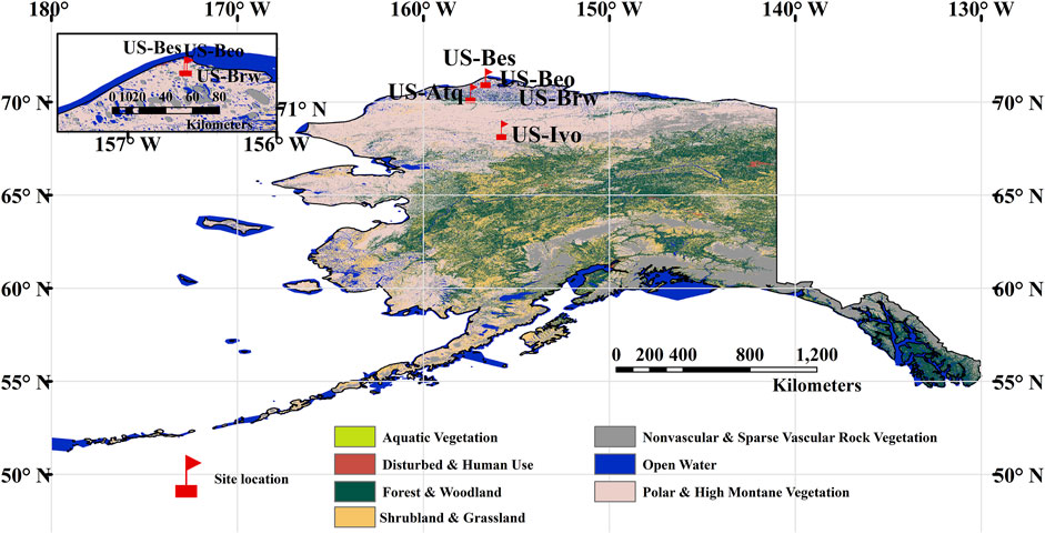
FIGURE 1. The land cover in Alaskan region and an inset showing the location of the eddy covariance tower sites and National Oceanic and Atmospheric Administration (NOAA) BRW station in Alaska. The land cover in Alaskan region was from GAP/LANDFIRE National Terrestrial Ecosystems data for U.S. and provided by the United States Geological Survey (https://www.usgs.gov/). The US-Brw, US-Bes, and US-Beo are overlapped as three sites are close in distance; two-site labels are shown in the inset.
2.1.2 Data Source
CH4 flux was monitored at a half-hourly time step using an EC tower at each study site for the period of 2013–2015, and half-hourly flux was calculated from raw data using the EddyPro software by LI-COR while missing data were gap-filled (Oechel and Kalhori, 2018). Winter CH4 flux was difficult to monitor due to the frozen equipment and frozen soil (Goodrich et al., 2016; Zona et al., 2016). Daily CH4 flux was calculated as the mean of half-hourly EC flux. Detailed information about the measurement protocols is available at https://daac.ornl.gov/ABOVE/guides/AK_North_Slope_NEE_CH4_Flux.html.
2.2 Model Implementation
2.2.1 Model Description and Driving Data
The CLM-Microbe model branches from the framework of default CLM 4.5 in 2013. Therefore, the CLM-Microbe has default decomposition subroutines in CLM4.5 (Thornton and Rosenbloom, 2005; Thornton and Zimmermann, 2007; Koven et al., 2013). The improvements in the CLM-Microbe model include a new microbial-functional-group-based CH4 module (Xu et al., 2015; Wang et al., 2019), and a new framework for microbial controls on carbon mineralization (Xu et al., 2014; He et al., 2021b). Detailed mathematical expressions for CH4 production, consumption, and transport processes were organized (Xu et al., 2015; Wang et al., 2019). The code for the CLM-Microbe model has been archived at https://github.com/email-clm/CLM-Microbe since 2015. The model version used in this study was obtained from GitHub on 27 May 2020.
The CLM-Microbe model considers the dynamics of dissolved organic carbon, acetate, O2, H2, CH4, CO2, and the processes of fermentation, homoacetogenesis, methanogenesis, and methanotrophy (Xu et al., 2015). The four key mechanisms for CH4 production and consumption are methanogenesis from acetate or from single-carbon compounds; CH4 oxidation using molecular oxygen or other inorganic electron acceptors; and four microbial functional groups perform these processes: acetoclastic methanogens, hydrogenotrophic methanogens, aerobic methanotrophs, and anaerobic methanotrophs (Xu et al., 2015; Wang et al., 2019). The soil profile is the same as the CLM4.5 (Oleson et al., 2013).
In our previous study (Wang et al., 2019), this module was validated with incubation flux and closed-chamber flux and further compared with EC flux using an area-weighted average approach for upscaling. In this study, we considered the spatial heterogeneity of vegetation and elevation within the EC domain for each study site and conducted the model simulations at a spatial resolution of 4 m × 4 m with a domain of 40,000 m2 with the EC tower at the center. Meteorological variables driving the model include shortwave and longwave radiation, air temperature, relative humidity, wind speed, and precipitation. US-Beo, US-Bes, and US-Brw shared the same meteorological parameters due to the small distance between sites, which were generated by Xu and Yuan (2016) for the period of 1991–2015 and can be obtained from the Utqiaġvik, AK, station of NOAA/Earth System Laboratory, Global Monitoring Division (http://www.esrl.noaa.gov/gmd/obop/brw/). The data set is gap-filled and at a half-hourly time step. Meteorological variables for US-Atq and US-Ivo were extracted from the half-hourly, gap-filled CRUNCEP dataset version 4.0 with a resolution of 0.5° × 0.5° longitude/latitude resolution for a period of 1991–2014 (https://rda.ucar.edu/datasets/ds314.3/).
Other model parameters include spatial distribution of vegetation and a digital elevation model with a resolution of 4 m covering the tower domain at each site, and soil organic carbon (SOC) concentration at ten soil layers defined in CLM4.5 (Thornton and Rosenbloom, 2005; Thornton et al., 2007; Koven et al., 2013). The vegetation distribution in the source area for US-Brw, US-Beo, and US-Bes was determined using a random forest algorithm using the plant functional type (PFT) from Langford et al. (2019) as training data (Supplementary Figure S2). Four PFTs were classified among five areas, including Arctic C3 grass, bare soil, broadleaf evergreen shrub, and broadleaf deciduous boreal shrub. The former three PFTs dominated and accounted for >80% of the domain of each area. A World-View3 image (Maxar Technologies) of the Barrow areas collected on July 24, 2016, was used with the plant functional type map overlaid to predict plant functional types at the other Barrow sites. The model was trained by using 1,000 pixels at random and then applied the trained models to the World-View3 image near the sites of interest. For the US-Atq and US-Ivo sites, an unsupervised linear spectral unmixing was performed in ENVI V5.2 (L3Harris Geospatial) using the vegetation classes from a previous publication (Davidson et al., 2016) to inform the number of classes, with an additional open water category. Following the unmixing, vegetation classes were applied according to (Davidson et al., 2016). A 0.5 m (vertical resolution) digital elevation model (DEM) was used for elevation data at the US-Beo, US-Bes, and US-Brw sites (Wilson, 2012). The elevation maps for US-Atq and US-Ivo were downloaded from ArcticDEM (v3.0 Pan-Arctic) with a high resolution of 2 m based on the geographic information of these two sites and further processed to maps with a resolution of 4 m using the MATLAB software (R2018a, the MatWorks, Inc.). SOC concentrations at 0–10, 10–20, 20–30, and 30–40 cm at US-Bes, US-Atq, and US-Ivo were derived from the Northern Circumpolar Soil Carbon Database (Hugelius et al., 2013). Due to the lack of SOC data, we assumed that US-Beo and US-Brw shared the same SOC data as BES since these sites are adjacent. In addition, since there was no spatial data of SOC, we assumed that all the grid cells within a domain of 40,000 m2 had the same vertical distribution of SOC. To calculate SOC at each soil layer for model simulation, we assumed the cumulative SOC fraction follows an asymptotic equation (Jackson et al., 1996; Xu et al., 2013; Guo et al., 2020); therefore, SOC concentration for each soil layer was estimated by an exponential equation:
where the Y is SOC concentration at the soil depth d (m) and a and β are the fitted “coefficient” (Supplementary Table S1). The SOC dataset used for model simulation was shown in Table 1.
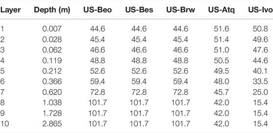
TABLE 1. Concentration of soil organic carbon (SOC) (kg C m−3) for model initialization for all study sites.
2.2.2 Model Implementation
Model implementation was carried out in three stages, similar to the default CLM4.5 protocols (Oleson et al., 2013). The first phase is an accelerated model spin-up that was set up for 2,000 years to allow the system to accumulate C and reach a steady state. We set the accelerated model spin-up for 2,000 years to allow more carbon accumulation as the Arctic tundra has a low rate and long period of carbon sequestration. Then a final spin-up was set up for 50 years to allow the modeled system to reach a relatively steady state. After the final spin-up, the transient model simulation was set to cover the period of 1850–2015 for US-Beo, US-Bes, and US-Brw, and the period of 1850–2014 for US-Atq and US-Ivo. The difference in model duration was determined by the available meteorological data for each site. The climate data of 1850–2015 and 1850–2014 were covered as the CLM-Microbe model can be set to cycle the extant climate data.
For the model simulations, parameters for microbial community and hydrological processes were set to default values in the CLM-Microbe model for each study site (Oleson et al., 2013; Xu et al., 2015; Wang et al., 2019). To simulate the actual hydrological processes in this area, we modified the soil hydrology module and changed parameters for the inundated fraction to guarantee soil inundated below the 5th soil layer (2 m) in the CLM-Microbe model. In addition, the parameters for plant-mediated transport of CH4 were changed to allow CH4 emission from soil. The transient simulations for each site produced output at the daily time step. The same model parameters and settings were applied for all five study sites.
2.2.3 Footprint Algorithms
In this study, we upscaled the simulated CH4 flux to the landscape scale using three footprint algorithms. The first algorithm was the “homogeneous” footprint (HF) algorithm, which assumes the footprint is a circular area with a radius of 100 m and the EC tower as the center and each grid cell in the footprint contributes equally (Figure 2A). The second algorithm was the “gradient” footprint (GF) algorithm, which assumes the footprint is also a circle area with a radius of 100 m and the EC tower as the center, but grid cells contribute distinctly and their contribution weights decrease from 1 at the center to 0 at the edge in the footprint (Figure 2B). Both HF and GF were constant over time. The third algorithm was the “dynamic” footprint (DF) algorithm, which considered the influence of wind direction, wind velocity, air temperature, sensible heat, precipitation, and the landscape roughness to rigorously characterize the actual EC footprint (Chen et al., 2012; Kim et al., 2006; Kormann and Meixner, 2001) (Figure 2C). The DF was developed to estimate the probability of flux originating from a particular location surrounding the flux tower (Chen et al., 2012).
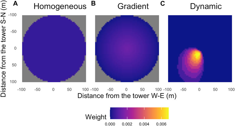
FIGURE 2. Source area and weight distribution for different footprint algorithms within an area of 200 m × 200 m and the EC tower as the center (50 latitude grids × 50 longitude grids): (A) the “homogeneous” footprint (HF) algorithm regards each grid cell contributes evenly to total EC flux, (B) the “gradient” footprint (GF) algorithm regards the contribution of grid cells gradually decrease from the center to edge; and (C) the “dynamic” footprint (DF) algorithm considers the environmental influence to generate dynamic EC footprints at daily time step. Figure (A) and (B) are constant throughout the year. Figure (C) shows a sample of EC footprints produced for ATQ on 22 September 2013. Grey indicates the data are unavailable. Relative weights are shown and the weights for all grids within the entire domain sum to one.
We produced the footprint with HF and GF algorithms using R, version 3.6 (R Core Team, 2020) and implemented the DF following the protocols using the MATLAB software (R2018a, MatWorks, Inc.) (Kormann and Meixner, 2001). The DF was generated at a daily time step and only for the days with no precipitation. Meteorological data for the DF were derived by the EC technique, including friction velocity, crosswind covariance, Monin-Obukhov length, roughness length, displacement height, and wind direction available at the half-hourly time step for the period of 2013–2015 (https://daac.ornl.gov/ABOVE/guides/AK_North_Slope_NEE_CH4_Flux.html).
2.2.4 Model Evaluation
Model evaluation was performed for the combined use of the CLM-Microbe model with each footprint model. The upscaled flux was calculated by the grid-cell CH4 flux and its weight in the footprint and validated with the measured EC flux in 2013–2015 for each site. The coefficient of determination (R2) and root mean square error (RMSE) were calculated for comparing upscaled and observed daily CH4 flux at monthly and annual time steps using R, version 3.6 (R Core Team, 2020). The coefficients cannot be calculated for all months because of insufficient observations and limited DF. To further quantify the model accuracy, we adopted an index of Normalized Nash-Sutcliffe Efficiency (NNSE). The t is the time series of data, T is the total sample size, and Qo and Qm are the observed and modeled data, respectively. The NNSE has a range of [0, 1], and higher values indicate better model performance. It is noted that the NNSE is different from R2 as the NNSE takes heavy consideration of absolute values of individual data points, while R2 relies on the covariance between observational data and modeled outputs.
2.2.5 Statistical Analysis
Annual estimates of CH4 flux at each site were calculated based on observed and upscaled flux. Because some observed flux and DF estimates were missing, we interpolated those data with a linear method at daily time scales using R, version 3.6 (R Core Team, 2020). This approach has been applied to gap-fill the missing data, ranging from 10% for US-Beo, 21% for US-Bes, 42% for US-Brw, 43% for US-Atq, and 24% for US-Ivo. Additionally, in the current version of the CLM-Microbe model, CH4 emission does not occur when the surface water is frozen. Hence, we only used the flux for the period from DOY (day of the year) 121 to DOY 280 for annual estimates for all study sites. Therefore, annual CH4 flux for those areas can be underestimated by the mode since cold season flux can contribute up to 50% of annual flux (Zona et al., 2016). We also investigated the effects of air temperature, precipitation, vegetation composition, and elevation on temporal and spatial variations of CH4 flux for each site. A correlation analysis was conducted for quantify the effects of daily air temperature and precipitation on daily CH4 flux in 2013–2015. Correlations between vegetation composition and elevation and CH4 flux were analyzed based on the spatial distribution of those variables in 2013–2015. Pearson’s correlation coefficients (rp) are shown in Table 4 and Supplementary Table S5. All statistical analyses were conducted using R scripts developed in-house (version 3.6).
3 Results
3.1 Simulated CH4 flux Based on Footprint Algorithms
Compared with EC measurements, the estimates using DF algorithm were similar to those using HF and GF across study sites in 2013–2015, with an R2 range of 0.210–0.629 (Supplementary Table S3, Supplementary Figure S1). A total of 61–63% of the variations in observed flux were explained by the simulated flux at US-Bes and US-Atq using different footprint algorithms, while only 21% was explained for US-Ivo (Supplementary Table S3, Supplementary Figure S1). Values of RMSE were comparably small (0.008–0.011 μmol m−2 s−1) for all sites, except 0.023 at US-Ivo (Supplementary Table S3). At the monthly scale, the temporal variations of simulated CH4 flux were improved using the DF algorithm compared with HF and GF algorithms, especially in the summer months (July–September), whereas the accuracy of estimates was similar using the HF and GF algorithms (Table 2). In the months when the DF algorithm performed better, the correlation (R2) between observed and modeled flux was greatly increased compared with HF and GF algorithms (Table 2). However, we also observed a decreased accuracy of 36% using the DF algorithm compared with HF and GF algorithms at US-Ivo in September 2013. In the majority of the study period, the accuracy of estimated CH4 flux was consistent among DF, HF, and GF algorithms as shown by the similar NNSE values among the three algorithms (Table 2). Overall, the three footprint algorithms were consistent for all sites (Table 2). For instance, the NNSE value was 0.758 for the HF algorithm, 0.765 for the GF algorithm, and 0.782 for the DF algorithm at the US-Bes site in September 2013, indicating a slightly better performance of the DF algorithm than the other two algorithms.
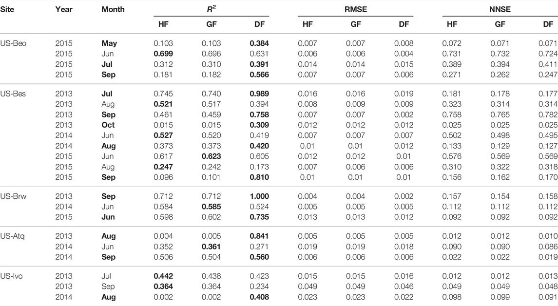
TABLE 2. Coefficients for simulated daily CH4 flux for each month using the homogeneous footprint (HF), gradient footprint (GF) and dynamic footprint (DF) algorithms compared with observed flux for all study sites. (RMSE: root mean square error; Bolded values are significant at p = 0.5; NNSE: the Normalized Nash-Sutcliffe Efficiency).
3.2 Simulated CH4 flux Among Study Sites
The CLM-Microbe model captured the starts, peaks, and seasonal trajectory of CH4 flux across study sites using different footprint algorithms (Figure 3). US-Beo, US-Bes, and US-Brw showed similar trends for CH4 emission with comparable average daily flux, even with different footprints in 2015 (Figure 3). The average CH4 flux of the growing seasons (DOY 121–280) at these three sites was in a range of 0.017–0.020 μmol m−2 s−1 in 2015. US-Atq and US-Ivo had higher average flux than US-Bes and US-Brw across footprints in 2013–2014. The average CH4 flux at US-Atq was 0.020 μmol m−2 s−1 in 2013, and 0.019 μmol m−2 s−1 in 2014 using different footprints. At US-Ivo, the average CH4 flux in 2013–2014 was 0.036–0.037 μmol m−2 s−1 using HF and GF algorithms, and 0.040–0.051 μmol m−2 s−1 using the DF algorithm.
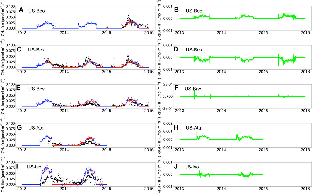
FIGURE 3. Left column shows the comparison of upscaled CH4 flux using the homogeneous footprint (HF) algorithm (green points), the gradient footprint (GF) algorithm (blue points) and the dynamic footprint (DF) algorithm (red points) with the EC observed flux (black points) for (A) US-Beo, (C) US-Bes, (E) US-Brw, (G) US-Atq, and (I) US-Ivo at daily time step during a period of 2013–2015. The right column shows the differences of CH4 flux between GF and HF for (B) US-Beo, (D) US-Bes, (F) US-Brw, (H) US-Atq, and (J) US-Ivo.
Annual estimates of upscaled CH4 flux were comparable using different footprints for each study site in the same year with a range of 3.0–8.3 g C m−2 (Table 3). Moreover, annual estimates of upscaled CH4 flux were consistent with estimates of observed flux for US-Beo and US-Bes in 2015 but were overestimated for US-Brw, US-Atq, and US-Ivo in 2014–2015. A small difference in annual estimates of CH4 flux was found among US-Beo, US-Bes, and US-Brw with a range of 3.7–4.3 g C m−2 using different footprint algorithms in 2015. Annual flux at US-Atq was overestimated as 4.0 g C m−2 by all footprint algorithms, which was 2.4 times the observed flux. In addition, the annual estimate of observed flux at US-Ivo in 2014 was 4.6 g C m−2, which was overestimated by 1.67–1.8 times using footprint algorithms (Table 3).

TABLE 3. Annual estimates of observed and upscaled CH4 flux using the homogeneous footprint (HF), gradient footprint (GF) and dynamic footprint (DF) algorithms for all study sites in 2013–2015 (Unit: g C m−2 year−1, n.a.: not available).
3.3 Spatial Patterns of Simulated CH4 flux Within Study Domains
Spatial patterns of simulated CH4 flux varied among study sites at annual and monthly scales using different footprints (Figure 4 and Supplementary Figures S3–S19, Supplementary Table S4). Generally, the spatial variations were greatest using the HF algorithm across sites, which were 1.6 times of using the GF algorithm and 3.2–28 times of using the DF algorithm (Supplementary Table S4). Similar to spatial variations, spatial averages for each study site using the GF and DF algorithms were comparable but were about half of spatial averages using the HF algorithm (Supplementary Table S4). US-Ivo had the highest spatial averages compared with other sites (unit = µmol m−2 s−1): 0.0125–0.129 using the HF algorithm, 0.0044–0.0046 using the GF algorithm, and 0.0012–0.0017 using the DF algorithm (Figure 4, Supplementary Figures S3, S4, Supplementary Table S4). US-Atq had the second-highest spatial averages and variations (unit = µmol m−2 s−1): 0.0062–0.0069 using the HF algorithm, 0.0022–0.0025 using the GF algorithm, and 0.0002–0.0004 using the DF algorithm (Figure 4, Supplementary Figures S3, S4, Supplementary Table S4). US-Beo, US-Bes, and US-Brw had similar spatial averages using different footprint algorithms, which were 0.0047–0.0007 using the HF algorithm, 0.0016–0.0024 using the GF algorithm, and 0.0001–0.0005 using the DF algorithm (Figure 4, Supplementary Figures S3, S4, Supplementary Table S4). Spatial patterns of CH4 flux were scaled up by three footprint algorithms (Figure 4, Supplementary Figures S3, S4), but they cannot be verified because there is no available observation for spatial distribution of CH4.
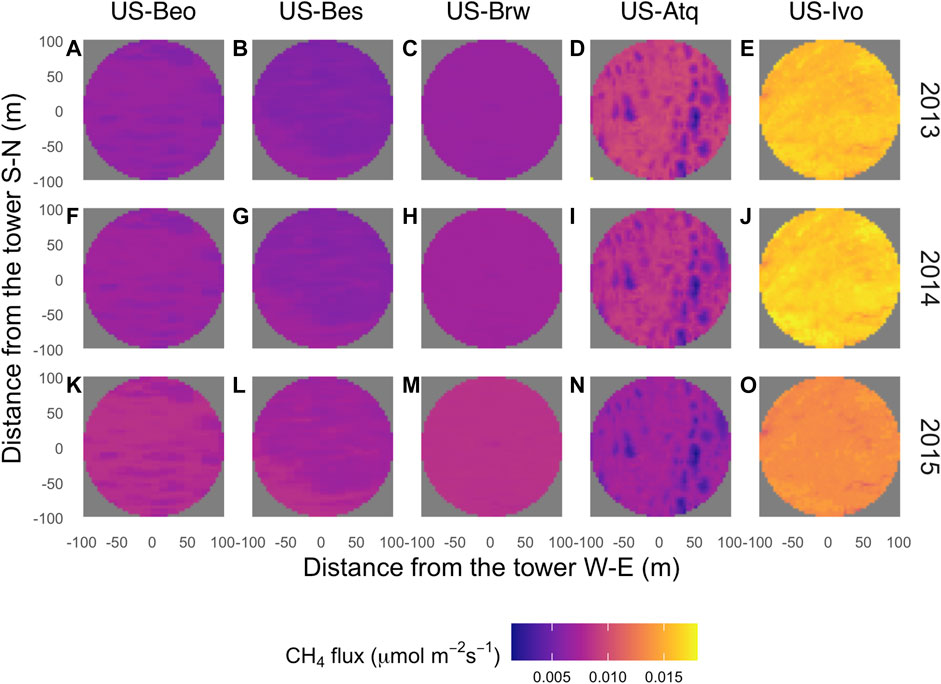
FIGURE 4. Spatial patterns of upscaled CH4 emission rates based on the homogeneous footprint (HF) algorithm in an area of 200 m × 200 m during a period of 2013–2015 for (A, F, K) US-Beo, (B, G, L) US-Bes, (C, H, M) US-Brw, (D, I, N) US-Atq, and (E, J, O) US-Ivo.
3.4 Controls on the Variations in CH4 flux
Air temperature and precipitation were the primary factors determining CH4 flux at the temporal scale (Table 4). The influences of air temperature and precipitation on CH4 flux were highly dependent on footprint algorithms across study sites. In summary, air temperature explained 67.3–74.3% whereas precipitation explained 22.3–35.6% of the temporal variations in CH4 flux among the five study sites (Table 4). At the spatial scale, CH4 flux was negatively correlated with bare soil percentage and positively correlated with Arctic C3 grass percentage using different footprint algorithms among the five sites, except for US-Bes; in other words, higher vegetation cover was associated with greater CH4 emission (Supplementary Table S5). Arctic C3 grass percentage was strongly related to CH4 flux at US-Beo using the HF (rp = 0.385, p < 0.0001), GF (rp = 0.284, p < 0.0001) and DF (rp = 0.265, p < 0.0001) algorithms; at US-Atq using the HF (rp = 0.718, p < 0.0001), GF (rp = 0.305, p < 0.0001) and DF (rp = 0.280, p < 0.0001) algorithms; and at US-Bes (rp = 0.488, p < 0.0001) and US-Ivo (rp = 0.305, p < 0.0001) using the HF algorithm. More Arctic C3 grasses facilitated CH4 emission among five study sites (Supplementary Table S5). Generally, soil temperature and soil water content were positively correlated with CH4 fluxes using different footprint algorithms (Supplementary Table S5); however, their correlations seemed to be overlaid by Arctic C3 grass and bare soils. CH4 fluxes were positively correlated with soil temperature (rp = 0.265, p < 0.0001) and soil water content (rp = 0.249, p < 0.0001), but these direction of correlation was changed using GF (rp = -0.242, p < 0.0001 for soil temperature; rp = -0.210, p < 0.0001 for soil water content) and DF (rp = -0.229, p < 0.0001 for soil temperature; rp = -0.200, p < 0.0001 for soil water content) algorithms (Supplementary Table S5).
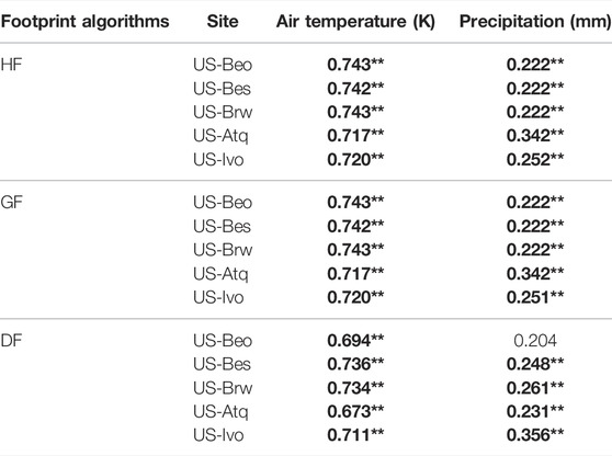
TABLE 4. Pearson’s correlation coefficients (rp) for relationships between air temperature, precipitation and upscaled CH4 flux using the homogeneous footprint (HF), gradient footprint (GF) and dynamic footprint (DF) for all study sites (Bold indicates | rp | > 0.2; * indicates p < 0.05, **p < 0.01).
4 Discussion
4.1 Importance of Footprint Algorithms in Upscaling CH4 Emission to the Landscape Scale
In this study, we integrated three footprint algorithms with a microbial functional group-based CH4 model for upscaling plot-scale CH4 flux to the landscape scale. Generally, the simulated flux was consistent with the observed CH4 flux at the five study sites during 2013–2015 (Figure 3). This confirmed that the CLM-Microbe model is capable of simulating the temporal pattern of landscape-scale CH4 emission in Arctic tundra (Wang et al., 2019). Additionally, Arctic tundra (about 11,563,300 km2) was estimated to emit 7.54–20.87 Tg CH4 per year based on our maximum and minimum annual estimates using different footprints among all study sites, which were comparable to previous estimates (Zona et al., 2016). However, our model generally overestimated CH4 emissions for US-Brw, US-Atq, and US-Ivo in 2014–2015 and underestimated flux for US-Bes in 2014, regardless of footprint algorithms (Table 2). GF and DF algorithms narrowed the discrepancies between simulated and observed flux for US-Ivo compared with the HF algorithm, and their effects were small, and upscaled fluxes were still 1.67–1.78 times annual estimates of observed flux. It is probably due to the relatively homogeneous surface of the source area, which led to small spatial variations in CH4 flux at US-Ivo and further weakened the influence of footprints on upscaled fluxes (Figure 4).
The footprint algorithms can be a key factor for the regional quantification of the CH4 flux. For example, at US-Bes in September 2013, the R2 of the DF algorithm was almost double the R2 for the GF algorithm. This is because the upscaled flux can be simulated to be zero using the GF algorithm, which can lead to a huge difference between measured and upscaled data. But upscaled flux using the DF algorithm can only be calculated when the measured flux is not zero, which guarantees that the upscaled flux using the DF algorithm would not be zero and may be close to the measured flux. This is why the differences in upscaled flux between the DF algorithm and the GF algorithm seem to be tiny in Figure 3, but the R2 using DF and GF can be largely different in Table 3. Previous research found that footprint algorithms were of considerable importance for improving greenhouse gas budgeting (Kljun et al., 2015; Chi et al., 2021), and footprints provide useful information about the spatial representativeness of flux in the case that footprint size and position determine the distribution of individual sinks or sources in the study areas with large heterogeneity (Heidbach et al., 2017; Reuss-Schmidt et al., 2019; Chu et al., 2021). Thus, it is reasonable to have a small effect of footprints on improving CH4 estimates in homogenous areas, suggesting that footprint estimates are more important when validating CH4 emission models with EC fluxes for areas with a heterogeneous and irregular vegetation pattern (Budishchev et al., 2014). A study reported the footprint for 214 AmeriFlux sites and found that upscaling with a fixed-extent target area can lead to up to 20% of biases. A recent review paper highly recommended the footprint algorithm as a key task for the flux community (Helbig et al., 2021). This study added another piece of evidence of the importance of dynamic footprint in predicting CH4 flux at the regional scale.
The footprint algorithms varied among temporal scales; for example, the DF algorithm had better performance in upscaling the CH4 flux at the monthly scale than at the annual scale. The DF algorithm performed better or comparable to improve the accuracy of CH4 annual estimates compared with the HF and GF algorithms. The HF and GF algorithms were immutable over time, whereas the DF algorithm considers the impact of turbulence in releasing CH4 from ecosystems (Kljun et al., 2015). Strong atmospheric turbulence can facilitate the instantaneous release of CH4 bubbles trapped within the soil or on surfaces below the water table (Sturtevant et al., 2012). Moreover, friction velocity, which is strongly correlated with wind speed, has been reported to be positively correlated to CH4 emission in Arctic and sub-Arctic tundra (Sachs et al., 2008; Sturtevant et al., 2012). The DF algorithm performed better in summer months (July–September). This may be explained by the enhanced preformation of dynamic footprint estimates over heterogeneous ground, and in summer months the unstable conditions of atmospheric turbulence and vegetation cause a higher spatial heterogeneity than in winter (Sturtevant et al., 2012).
4.2 Factors Controlling Landscape-Scale CH4 Emission
In this study, the air temperature was the dominant factor controlling CH4 emission in the Arctic tundra, which explained 67.3–74.3% of the temporal variation in CH4 flux. Three study sites in Utqiaġvik (US-Beo, US-Bes, and US-Brw) exhibited the same trend, start, peak, and end of CH4 emission since they experienced the same climate conditions (Figure 3). The annual average air temperature was highest at US-Ivo, the southernmost study site, which correspondingly had the greatest CH4 emission (Arndt et al., 2019; Arndt et al., 2020). The key role of temperature affecting Arctic CH4 emission has been illustrated in numerous studies (Morrissey and Livingston, 1992; Chistensen, 1993; Christensen and Cox, 1995; Christensen et al., 2004; Nielsen et al., 2017): 1) warmer temperature leads to a deeper active layer, allowing a greater soil volume to produce CH4; 2) temperature directly affects microbial activities and efficiency of converting substrates to produce CH4, and 3) temperature influences the plant growth and biomass in the ecosystem that impacts CH4 transport via plants. Further, precipitation explained 22.3–35.6% of the temporal variations in CH4 flux among different sites. This is because CH4 is produced by methanogens in inundated soils with no oxygen, and is oxidized in soils above the water table or in while diffusing through open water (MacDonald et al., 1998).
Spatial variations of CH4 emission were influenced by vegetation distribution in Arctic tundra ecosystems. Higher vegetation cover was associated with larger CH4 emissions within study sites due to the stronger plant-mediated transport of CH4 (Waddington and Roulet, 1996; King et al., 1998). In contrast, the US-Bes displayed a positive relationship between non-vegetation proportion and CH4 emission within the source area, which may be because inundated areas inhibited plant growth, but accelerated ebullition and production of CH4. C3 grasses dominate the landscape of the Arctic tundra and are known to provide a conduit for CH4 to transport to the atmosphere. As a result, CH4 emissions are strongly correlated with vascular species cover and root density (Joabsson and Christensen, 2001; Sturtevant et al., 2012; Davidson et al., 2016). Further, Bellisario et al. (1999) found an inverse relationship between water table position and CH4 flux in a Canadian northern peatland, and a greater vascular plant cover was most responsible for higher emissions. A few comprehensive analyses with the FLUXNET-CH4 data have confirmed the substrate and water table as key controlling factors for CH4 flux (Chang et al., 2021; Delwiche et al., 2021; Knox et al., 2021). More mechanistic analysis with our model for quantitative understanding of those factors on CH4 flux is deemed as future work.
Combining the controls on temporal and spatial variations in CH4 flux, we found that climate and seasonal drivers dominated the temporal variability while the spatial heterogeneity in land surface property dominated the spatial variability in CH4 flux. This is consistent with two studies in the Arctic (Treat et al., 2018; Hashemi et al., 2021). Considering the small differences among the three algorithms in upscaling CH4 flux, it suggested that the variation in CH4 flux over months is larger than that of the variation across space in the Arctic (Hashemi et al., 2021), indicating that maybe the coarser scale models are suitable in capturing total budget but not finer scale temporal rends in the Arctic (Melton et al., 2013).
4.3 The Implications
This study has three major implications for model development and upscaling CH4 emissions in the Arctic. First, the CLM-Microbe model performed well in capturing the temporal variability in CH4 flux among different landscapes in the Arctic tundra, thereby improving the simulation accuracy for CH4 flux with appropriate footprint algorithms. This study infers that the DF algorithm had similar performance to HF and GF algorithms if the landscape is flat. Second, this study emphasizes the importance of vegetation composition in influencing the spatial heterogeneity of CH4 emission in agreement with many prior studies (Waddington and Roulet, 1996; McEwing et al., 2015; Davidson et al., 2016). However, the proportions of different plant function types are defined as unchanged during model simulation. The CLM-Microbe model could improve estimates by developing a more advanced vegetation module to improve the simulation performance for vegetation effects on CH4 flux that have been observed to change over decadal timescales (Liljedahl et al., 2016; Arndt et al., 2019). Third, this study infers the importance of topography in driving CH4 flux across the heterogeneous landscape. This study adopted a spatial resolution of 4 m × 4 m for the tower domain, yet soil heterogeneity is observed within a sub-meter scale. Finer resolution of soil and vegetation data might be critical for better simulating CH4 flux at a sub-meter scale in Arctic tundra landscapes.
4.4 The Way Forward
Previous and current results demonstrate the robustness of the CLM-Microbe model to simulate the landscape-scale CH4 emission in the Arctic tundra by incorporating different upscaling techniques (Wang et al., 2019). Here we identify several tasks required to further advance the modeling of landscape-level CH4 emission in Arctic tundra. First, CH4 emission during the cold season is very important, which possibly contributes up to ∼50% of annual estimates in Arctic tundra (Zona et al., 2016; Arndt et al., 2020; Hashemi et al., 2021). The formation of a zero curtain during the cold season thereby contributes to a large underestimation of CH4 production (Mastepanov et al., 2008; Mastepanov et al., 2013; Zona et al., 2016). The current version of CLM-Microbe allows CH4 release from a frozen soil surface, and the model does not effectively simulate the CH4 dynamics associated with the zero-curtain in Arctic tundra. Hence, a more accurate representation of the actual soil hydrological and physical condition is warranted. Second, estimation of the Arctic CH4 budget can be improved by the CLM-Microbe model, owing to the simulation of different microbial functional groups (methanogens vs methanotrophs) acting in CH4 processes. Based on the current study, it is feasible to conduct the model simulation of CH4 for Arctic regions using the Circumpolar Arctic map. Extrapolating to the entire Arctic by combining relatively high-resolution vegetation maps and topography data would tremendously improve the accuracy of the CH4 emission estimates. Third, the “hot moments” may represent a disproportionate contribution to the annual CH4 flux in the permafrost region (Song et al., 2012; Mastepanov et al., 2013; Pirk et al., 2015; Raz-Yaseef et al., 2016), yet no landscape and regional modeling studies have fully taken it into consideration these “hot moments” events (Xu et al., 2016). Although our model showed a high pulse in the early growing season, more mechanistic evaluation of the CH4 pulse dynamics should be included in our future work. Fourth, the selection of footprint algorithms for upscaling plot-level CH4 flux is important for landscape-scale CH4 estimates. Currently, various models have been used to estimate the source area of flux measurements (Zhang et al., 2012; Budishchev et al., 2014). This study compared three footprint algorithms for upscaling CH4 flux. Other footprint algorithms such as Lagrangian particle models (Heidbach et al., 2017) and the development of complex “full flow” large-eddy simulations may need to be considered for a more comprehensive evaluation.
5 Conclusion
This study reported applying the CLM-Microbe model to landscape-scale CH4 emission in the Arctic tundra in association with three footprint algorithms. The model captured the temporal dynamics of CH4 emission for different study sites, even when using the same model settings and parameters. The DF algorithm improved the accuracy of temporal variations in CH4 flux compared with the HF and GF algorithms by considering the influence of wind and soil surface conditions. It performed better on a monthly scale than on an annual scale. Due to the relatively flat landscape in the Arctic, the three footprint algorithms did not lead to substantial differences in the magnitudes of observed CH4 flux within a portion of the study sites. Air temperature explained 67–74% of temporal variations of CH4 flux, whereas precipitation explained 22–36% of temporal variations. Concerning spatial dynamics, vegetation cover was positively related to Arctic CH4 emission from soil to the atmosphere. In particular, the C3 arctic grasses play an essential role in facilitating CH4 transport from soil to the atmosphere. Extrapolating our modeling results to the northern Arctic tundra ecosystems led to an annual CH4 emission of 7.54–20.87 Tg CH4 per year. This study suggests that the approach adopted in this study is applicable to other ecosystem types around the globe. The selection of an appropriate footprint model for upscaling CH4 flux depends on the landscape characteristics of the study domains.
Data Availability Statement
Publicly available datasets were analyzed in this study. This data can be found here: The data used in this study have been archived at five sites are available at https://daac.ornl.gov/ABOVE/guides/AK_North_Slope_NEE_CH4_Flux.html.
Author Contributions
XX conceived the project. YW prepared model driving forces and set up the model simulation, finished the analysis, and wrote up the paper with the assistance of XX. The model development and setup have been supported by FY, JL, LH, YZ, DR, and PT. The vegetation and elevation data were from KA. The soil organic carbon data were from DL. The methane flux data were from DZ, DL, WO, and SW. All authors interpreted the results.
Funding
Financial assistance was partially provided by the SPRUCE and NGEE Arctic projects, which are supported by the Office of Biological and Environmental Research in the Department of Energy Office of Science. This project is partially supported by the U.S. National Science Foundation (No. 1702797, 2145130). Geospatial support for this work was provided by the Polar Geospatial Center under NSF OPP awards 1204263 and 1702797.
Conflict of Interest
The authors declare that the research was conducted in the absence of any commercial or financial relationships that could be construed as a potential conflict of interest.
Publisher’s Note
All claims expressed in this article are solely those of the authors and do not necessarily represent those of their affiliated organizations, or those of the publisher, the editors and the reviewers. Any product that may be evaluated in this article, or claim that may be made by its manufacturer, is not guaranteed or endorsed by the publisher.
Acknowledgments
We are grateful to Randy A. Dahlgren from the University of California–Davis for his constructive suggestions in the early phase of this study. Dr. Johannes Laubach and three reviewers provided valuable suggestions that have significantly improved the manuscript. The authors are grateful for financial and facility support from San Diego State University.
Supplementary Material
The Supplementary Material for this article can be found online at: https://www.frontiersin.org/articles/10.3389/fenvs.2022.939238/full#supplementary-material
References
Andresen, C. G., Lara, M. J., Tweedie, C. E., and Lougheed, V. L. (2017). Rising Plant‐Mediated Methane Emissions from Arctic Wetlands. Glob. Change Biol. 23 (3), 1128–1139. doi:10.1111/gcb.13469
Arndt, K. A., Oechel, W. C., Goodrich, J. P., Bailey, B. A., Kalhori, A., Hashemi, J., et al. (2019). Sensitivity of Methane Emissions to Later Soil Freezing in Arctic Tundra Ecosystems. J. Geophys. Res. Biogeosci. 124 (8), 2595–2609. doi:10.1029/2019jg005242
Arndt, K. A., Lipson, D. A., Hashemi, J., Oechel, W. C., and Zona, D. (2020). Snow Melt Stimulates Ecosystem Respiration in Arctic Ecosystems. Glob. Change Biol. 26 (9), 5042–5051. doi:10.1111/gcb.15193
Baldocchi, D. (2008). 'Breathing' of the Terrestrial Biosphere: Lessons Learned from a Global Network of Carbon Dioxide Flux Measurement Systems. Aust. J. Bot. 56 (1), 1–26. doi:10.1071/bt07151
Bellisario, L. M., Bubier, J. L., Moore, T. R., and Chanton, J. P. (1999). Controls on CH4 Emissions from a Northern Peatland. Glob. Biogeochem. Cycl. 13 (1), 81–91. doi:10.1029/1998gb900021
Bhullar, G. S., Iravani, M., Edwards, P. J., and Olde Venterink, H. (2013). Methane Transport and Emissions from Soil as Affected by Water Table and Vascular Plants. BMC Ecol. 13 (1), 32–39. doi:10.1186/1472-6785-13-32
Budishchev, A., Mi, Y., van Huissteden, J., Belelli-Marchesini, L., Schaepman-Strub, G., Parmentier, F. J. W., et al. (2014). Evaluation of a Plot-Scale Methane Emission Model Using Eddy Covariance Observations and Footprint Modelling. Biogeosciences 11 (17), 4651–4664. doi:10.5194/bg-11-4651-2014
Chang, K.-Y., Riley, W. J., Knox, S. H., Jackson, R. B., McNicol, G., Poulter, B., et al. (2021). Substantial Hysteresis in Emergent Temperature Sensitivity of Global Wetland CH4 Emissions. Nat. Commun. 12 (1), 1–10. doi:10.1038/s41467-021-22452-1
Chen, B., Coops, N. C., Fu, D., Margolis, H. A., Amiro, B. D., Black, T. A., et al. (2012). Characterizing Spatial Representativeness of Flux Tower Eddy-Covariance Measurements across the Canadian Carbon Program Network Using Remote Sensing and Footprint Analysis. Remote Sens. Environ. 124, 742–755. doi:10.1016/j.rse.2012.06.007
Chi, J., Zhao, P., Klosterhalfen, A., Jocher, G., Kljun, N., Nilsson, M. B., et al. (2021). Forest Floor Fluxes Drive Differences in the Carbon Balance of Contrasting Boreal Forest Stands. Agric. For. Meteorol. 306, 108454. doi:10.1016/j.agrformet.2021.108454
Christensen, T. R., and Cox, P. (1995). Response of Methane Emission from Arctic Tundra to Climatic Change: Results from a Model Simulation. Tellus B Chem. Phys. Meteorol. 47 (3), 301–309. doi:10.3402/tellusb.v47i3.16049
Christensen, T. R., Johansson, T., Åkerman, H. J., Mastepanov, M., Malmer, N., Friborg, T., and Svensson, B. H. (2004). Thawing Sub‐arctic Permafrost: Effects on Vegetation and Methane Emissions. Geophys. Res. Lett. 31, L04501. doi:10.1029/2003gl018680
Christensen, T. R. (1993). Methane Emission from Arctic Tundra. Biogeochemistry 21 (2), 117–139. doi:10.1007/bf00000874
Chu, H., Luo, X., Ouyang, Z., Chan, W. S., Dengel, S., Biraud, S. C., et al. (2021). Representativeness of Eddy-Covariance Flux Footprints for Areas Surrounding AmeriFlux Sites. Agric. For. Meteorol. 301-302, 108350. doi:10.1016/j.agrformet.2021.108350
Davidson, S. J., Sloan, V. L., Phoenix, G. K., Wagner, R., Fisher, J. P., Oechel, W. C., et al. (2016). Vegetation Type Dominates the Spatial Variability in CH4 Emissions across Multiple Arctic Tundra Landscapes. Ecosystems 19 (6), 1116–1132. doi:10.1007/s10021-016-9991-0
Davidson, S., Santos, M., Sloan, V., Reuss-Schmidt, K., Phoenix, G., Oechel, W., et al. (2017). Upscaling CH4 Fluxes Using High-Resolution Imagery in Arctic Tundra Ecosystems. Remote Sens. 9 (12), 1227. doi:10.3390/rs9121227
Delwiche, K. B., Knox, S. H., Malhotra, A., Fluet-Chouinard, E., McNicol, G., Feron, S., et al. (2021). FLUXNET-CH4: a Global, Multi-Ecosystem Dataset and Analysis of Methane Seasonality from Freshwater Wetlands. Earth Syst. Sci. Data 13 (7), 3607–3689. doi:10.5194/essd-2020-307
Fox, A. M., Huntley, B., Lloyd, C. R., Williams, M., and Baxter, R. (2008). Net Ecosystem Exchange over Heterogeneous Arctic Tundra: Scaling between Chamber and Eddy Covariance Measurements. Glob. Biogeochem. Cycl. 22, GB2027. doi:10.1029/2007gb003027
Funk, D. W., Pullman, E. R., Peterson, K. M., Crill, P. M., and Billings, W. D. (1994). Influence of Water Table on Carbon Dioxide, Carbon Monoxide, and Methane Fluxes from Taiga Bog Microcosms. Glob. Biogeochem. Cycl. 8 (3), 271–278. doi:10.1029/94gb01229
Goodrich, J. P., Oechel, W. C., Gioli, B., Moreaux, V., Murphy, P. C., Burba, G., et al. (2016). Impact of Different Eddy Covariance Sensors, Site Set-Up, and Maintenance on the Annual Balance of CO2 and CH4 in the Harsh Arctic Environment. Agric. For. Meteorol. 228-229, 239–251. doi:10.1016/j.agrformet.2016.07.008
Guo, Z., Wang, Y., Wan, Z., Zuo, Y., He, L., Li, D., et al. (2020). Soil Dissolved Organic Carbon in Terrestrial Ecosystems: Global Budget, Spatial Distribution and Controls. Glob. Ecol. Biogeogr. 29 (12), 2159–2175. doi:10.1111/geb.13186
Hashemi, J., Zona, D., Arndt, K. A., Kalhori, A., and Oechel, W. C. (2021). Seasonality Buffers Carbon Budget Variability across Heterogeneous Landscapes in Alaskan Arctic Tundra. Environ. Res. Lett. 16 (3), 035008. doi:10.1088/1748-9326/abe2d1
He, L., Lai, C. T., Mayes, M. A., Murayama, S., and Xu, X. (2021a). Microbial Seasonality Promotes Soil Respiratory Carbon Emission in Natural Ecosystems: a Modeling Study. Glob. Change Biol. 27, 3035–3051. doi:10.1111/gcb.15627
He, L., Lipson, D. A., Mazza Rodrigues, J. L., Mayes, M., Björk, R. G., Glaser, B., et al. (2021b). Dynamics of Fungal and Bacterial Biomass Carbon in Natural Ecosystems: Site-Level Applications of the CLM-Microbe Model. J. Adv. Model. Earth Syst. 13, e2020MS002283. doi:10.1029/2020ms002283
Heidbach, K., Schmid, H. P., and Mauder, M. (2017). Experimental Evaluation of Flux Footprint Models. Agric. For. Meteorol. 246, 142–153. doi:10.1016/j.agrformet.2017.06.008
Helbig, M., Gerken, T., Beamesderfer, E. R., Baldocchi, D. D., Banerjee, T., Biraud, S. C., et al. (2021). Integrating Continuous Atmospheric Boundary Layer and Tower-Based Flux Measurements to Advance Understanding of Land-Atmosphere Interactions. Agric. For. Meteorol. 307, 108509. doi:10.1016/j.agrformet.2021.108509
Horst, T. W., and Weil, J. C. (1992). Footprint Estimation for Scalar Flux Measurements in the Atmospheric Surface Layer. Boundary-Layer Meteorol. 59 (3), 279–296. doi:10.1007/bf00119817
Hugelius, G., Tarnocai, C., Broll, G., Canadell, J. G., Kuhry, P., and Swanson, D. K. (2013). The Northern Circumpolar Soil Carbon Database: Spatially Distributed Datasets of Soil Coverage and Soil Carbon Storage in the Northern Permafrost Regions. Earth Syst. Sci. Data 5 (1), 3–13. doi:10.5194/essd-5-3-2013
Jackson, R. B., Canadell, J., Ehleringer, J. R., Mooney, H. A., Sala, O. E., and Schulze, E. D. (1996). A Global Analysis of Root Distributions for Terrestrial Biomes. Oecologia 108, 389–411. doi:10.1007/bf00333714
Joabsson, A., and Christensen, T. R. (2001). Methane Emissions from Wetlands and Their Relationship with Vascular Plants: an Arctic Example. Glob. Change Biol. 7 (8), 919–932. doi:10.1046/j.1354-1013.2001.00044.x
Kim, J., Guo, Q., Baldocchi, D., Leclerc, M., Xu, L., and Schmid, H. (2006). Upscaling Fluxes from Tower to Landscape: Overlaying Flux Footprints on High-Resolution (IKONOS) Images of Vegetation Cover. Agric. For. Meteorol. 136 (3-4), 132–146. doi:10.1016/j.agrformet.2004.11.015
King, J. Y., Reeburgh, W. S., and Regli, S. K. (1998). Methane Emission and Transport by Arctic Sedges in Alaska: Results of a Vegetation Removal Experiment. J. Geophys. Res. 103 (D22), 29083–29092. doi:10.1029/98jd00052
Kljun, N., Calanca, P., Rotach, M. W., and Schmid, H. P. (2015). A Simple Two-Dimensional Parameterisation for Flux Footprint Prediction (FFP). Geosci. Model Dev. 8 (11), 3695–3713. doi:10.5194/gmd-8-3695-2015
Knox, S. H., Bansal, S., McNicol, G., Schafer, K., Sturtevant, C., Ueyama, W. D., et al. (2021). Identifying Dominant Environmental Predictors of Freshwater Wetland Methane Fluxes across Diurnal to Seasonal Time Scales. Glob. Change Biol. 27, 3582–3604. doi:10.1111/gcb.15661
Kormann, R., and Meixner, F. X. (2001). An Analytical Footprint Model for Non-neutral Stratification. Boundary-Layer Meteorol. 99 (2), 207–224. doi:10.1023/a:1018991015119
Koven, C. D., Riley, W. J., Subin, Z. M., Tang, J. Y., Torn, M. S., Collins, W. D., et al. (2013). The Effect of Vertically Resolved Soil Biogeochemistry and Alternate Soil C and N Models on C Dynamics of CLM4. Biogeosciences 10, 7109–7131. doi:10.5194/bg-10-7109-2013
Kwon, H. J., Oechel, W. C., Zulueta, R. C., and Hastings, S. J. (2006). Effects of Climate Variability on Carbon Sequestration Among Adjacent Wet Sedge Tundra and Moist Tussock Tundra Ecosystems. J. Geophys. Res. Biogeosci. 111, G03014. doi:10.1029/2005jg000036
Lai, D. Y. F. (2009). Methane Dynamics in Northern Peatlands: A Review. Pedosphere 19 (4), 409–421. doi:10.1016/s1002-0160(09)00003-4
Langford, Z., Kumar, J., Hoffman, F., Norby, R., Wullschleger, S., Sloan, V., et al. (2016). Mapping Arctic Plant Functional Type Distributions in the Barrow Environmental Observatory Using WorldView-2 and LiDAR Datasets. Remote Sens. 8 (9), 733. doi:10.3390/rs8090733
Langford, Z. L., Kumar, J., Hoffman, F. M., Breen, A. L., and Iversen, C. M. (2019). Arctic Vegetation Mapping Using Unsupervised Training Datasets and Convolutional Neural Networks. Remote Sens. 11 (1), 69. doi:10.3390/rs11010069
Lara, M. J., McGuire, A. D., Euskirchen, E. S., Genet, H., Yi, S., Rutter, R., et al. (2020). Local-scale Arctic Tundra Heterogeneity Affects Regional-Scale Carbon Dynamics. Nat. Commun. 11 (1), 4925–5010. doi:10.1038/s41467-020-18768-z
Liljedahl, A. K., Boike, J., Daanen, R. P., Fedorov, A. N., Frost, G. V., Grosse, G., et al. (2016). Pan-Arctic Ice-Wedge Degradation in Warming Permafrost and its Influence on Tundra Hydrology. Nat. Geosci. 9 (4), 312–318. doi:10.1038/ngeo2674
MacDonald, J. A., Fowler, D., Hargreaves, K. J., Skiba, U., Leith, I. D., and Murray, M. B. (1998). Methane Emission Rates from a Northern Wetland; Response to Temperature, Water Table and Transport. Atmos. Environ. 32 (19), 3219–3227. doi:10.1016/s1352-2310(97)00464-0
Mastepanov, M., Sigsgaard, C., Dlugokencky, E. J., Houweling, S., Ström, L., Tamstorf, M. P., et al. (2008). Large Tundra Methane Burst during Onset of Freezing. Nature 456 (7222), 628–630. doi:10.1038/nature07464
Mastepanov, M., Sigsgaard, C., Tagesson, T., Ström, L., Tamstorf, M. P., Lund, M., et al. (2013). Revisiting Factors Controlling Methane Emissions from High-Arctic Tundra. Biogeosciences 10 (7), 5139–5158. doi:10.5194/bg-10-5139-2013
McEwing, K. R., Fisher, J. P., and Zona, D. (2015). Environmental and Vegetation Controls on the Spatial Variability of CH4 Emission from Wet-Sedge and Tussock Tundra Ecosystems in the Arctic. Plant Soil 388 (1-2), 37–52. doi:10.1007/s11104-014-2377-1
Melton, J. R., Wania, R., Hodson, E. L., Poulter, B., Ringeval, B., Spahni, R., et al. (2013). Present State of Global Wetland Extent and Wetland Methane Modelling: Conclusions from a Model Inter-comparison Project (WETCHIMP). Biogeosciences 10, 753–788. doi:10.5194/bg-10-753-2013
Mer, J. L., and Roger, P. (2001). Production, Oxidation, Emission and Consumption of Methane by Soils: a Review. Eur. J. Soil Biol. 37, 25–50. doi:10.1016/s1164-5563(01)01067-6
Morrissey, L. A., and Livingston, G. P. (1992). Methane Emissions from Alaska Arctic Tundra: An Assessment of Local Spatial Variability. J. Geophys. Res. 97 (D15), 16661–16670. doi:10.1029/92jd00063
Nielsen, C. S., Michelsen, A., Strobel, B. W., Wulff, K., Banyasz, I., and Elberling, B. (2017). Correlations between Substrate Availability, Dissolved CH4, and CH4 Emissions in an Arctic Wetland Subject to Warming and Plant Removal. J. Geophys. Res. Biogeosci. 122 (3), 645–660. doi:10.1002/2016jg003511
Oechel, W., and Kalhori, A. (2018). in ABoVE: CO2 and CH4 Fluxes and Meteorology at Flux Tower Sites, Alaska, 2015-2017. Oak Ridge, Ten, United States: ORNL DAAC. doi:10.3334/ORNLDAAC/1562
Oechel, W. C., Vourlitis, G. L., Brooks, S., Crawford, T. L., and Dumas, E. (1998). Intercomparison Among Chamber, Tower, and Aircraft Net CO2 and Energy Fluxes Measured during the Arctic System Science Land‐Atmosphere‐Ice Interactions (ARCSS‐LAII) Flux Study. J. Geophys. Res. 103 (D22), 28993–29003. doi:10.1029/1998jd200015
Oleson, K., Lawrence, D., Bonan, G. B., Drewniak, B. A., Huang, M., Koven, C. D., et al. (2013). Technical Description of Version 4.5 of the Community Land Model (CLM). Bounder, Colorado: National Center for Atmospheric Research.
Petrescu, A. M. R., Lohila, A., Tuovinen, J.-P., Baldocchi, D. D., Desai, A. R., Roulet, N. T., et al. (2015). The Uncertain Climate Footprint of Wetlands under Human Pressure. Proc. Natl. Acad. Sci. U.S.A. 112 (15), 4594–4599. doi:10.1073/pnas.1416267112
Pirk, N., Santos, T., Gustafson, C., Johansson, A. J., Tufvesson, F., Parmentier, F. J. W., et al. (2015). Methane Emission Bursts from Permafrost Environments during Autumn Freeze‐in: New Insights from Ground‐penetrating Radar. Geophys. Res. Lett. 42 (16), 6732–6738. doi:10.1002/2015gl065034
Pirk, N., Mastepanov, M., López-Blanco, E., Christensen, L. H., Christiansen, H. H., Hansen, B. U., et al. (2017). Toward a Statistical Description of Methane Emissions from Arctic Wetlands. Ambio 46 (1), 70–80. doi:10.1007/s13280-016-0893-3
R Core Team (2020). in R: A Language and Environment for Statistical Computing (Vienna, Austria). R.F.f.S. Computing.
Raz-Yaseef, N., Torn, M. S., Wu, Y., Billesbach, D. P., Liljedahl, A. K., Kneafsey, T. J., et al. (2016). Large CO2 and CH4 Emissions from Polygonal Tundra during Spring Thaw in Northern Alaska. Geophys. Res. Lett. 44, 504–513. doi:10.1002/2016GL071220
Reuss-Schmidt, K., Levy, P., Oechel, W., Tweedie, C., Wilson, C., and Zona, D. (2019). Understanding Spatial Variability of Methane Fluxes in Arctic Wetlands through Footprint Modelling. Environ. Res. Lett. 14 (12), 125010. doi:10.1088/1748-9326/ab4d32
Sachs, T., Wille, C., Boike, J., and Kutzbach, L. (2008). Environmental Controls on Ecosystem‐scale CH4 Emission from Polygonal Tundra in the Lena River Delta, Siberia. J. Geophys. Res. Biogeosci. 113, G00A03. doi:10.1029/2007JG000505
Serrano-Silva, N., Sarria-guzmán, Y., Dendooven, L., and Luna-Guido, M. (2014). Methanogenesis and Methanotrophy in Soil: a Review. Pedosphere 24 (3), 291–307. doi:10.1016/s1002-0160(14)60016-3
Song, C., Xu, X., Sun, X., Tian, H., Sun, L., Miao, Y., et al. (2012). Large Methane Emission upon Spring Thaw from Natural Wetlands in the Northern Permafrost Region. Environ. Res. Lett. 7 (3), 034009. doi:10.1088/1748-9326/7/3/034009
Sturtevant, C. S., and Oechel, W. C. (2013). Spatial Variation in Landscape‐level CO2 and CH4 Fluxes from Arctic Coastal Tundra: Influence from Vegetation, Wetness, and the Thaw Lake Cycle. Glob. Change Biol. 19 (9), 2853–2866. doi:10.1111/gcb.12247
Sturtevant, C. S., Oechel, W. C., Zona, D., Kim, Y., and Emerson, C. E. (2012). Soil Moisture Control over Autumn Season Methane Flux, Arctic Coastal Plain of Alaska. Biogeosciences 9 (4), 1423–1440. doi:10.5194/bg-9-1423-2012
Thornton, P. E., and Rosenbloom, N. A. (2005). Ecosystem Model Spin-Up: Estimating Steady State Conditions in a Coupled Terrestrial Carbon and Nitrogen Cycle Model. Ecol. Model. 189, 25–48. doi:10.1016/j.ecolmodel.2005.04.008
Thornton, P. E., and Zimmermann, N. E. (2007). An Improved Canopy Integration Scheme for a Land Surface Model with Prognostic Canopy Structure. J. Clim. 20, 3902–3923. doi:10.1175/jcli4222.1
Thornton, P. E., Lamarque, J. F., Rosenbloom, N. A., and Mahowald, N. M. (2007). Influence of Carbon-Nitrogen Cycle Coupling on Land Model Response to CO2 Fertilization and Climate Variability. Glob. Biogeochem. Cycl. 21 (4), GB4018. doi:10.1029/2006gb002868
Treat, C. C., Marushchak, M. E., Voigt, C., Zhang, Y., Tan, Z., Zhuang, Q., et al. (2018). Tundra Landscape Heterogeneity, Not Interannual Variability, Controls the Decadal Regional Carbon Balance in the Western Russian Arctic. Glob. Change Biol. 24 (11), 5188–5204. doi:10.1111/gcb.14421
Vaughn, L. J. S., Conrad, M. E., Bill, M., and Torn, M. S. (2016). Isotopic Insights into Methane Production, Oxidation, and Emissions in Arctic Polygon Tundra. Glob. Change Biol. 22 (10), 3487–3502. doi:10.1111/gcb.13281
von Fischer, J. C., Rhew, R. C., Ames, G. M., Fosdick, B. K., and von Fischer, P. E. (2010). Vegetation Height and Other Controls of Spatial Variability in Methane Emissions from the Arctic Coastal Tundra at Barrow, Alaska. J. Geophys. Res. Biogeosci. 115, G00I03. doi:10.1029/2009jg001283
Waddington, J. M., and Roulet, N. T. (1996). Atmosphere‐wetland Carbon Exchanges: Scale Dependency of CO2 and CH4 Exchange on the Developmental Topography of a Peatland. Glob. Biogeochem. Cycl. 10 (2), 233–245. doi:10.1029/95gb03871
Walker, D. A., Binnian, E., Evans, B. M., Lederer, N. D., Nordstrand, E., and Webber, P. J. (1989). Terrain, Vegetation and Landscape Evolution of the R4D Research Site, Brooks Range Foothills, Alaska. Ecography 12 (3), 238–261. doi:10.1111/j.1600-0587.1989.tb00844.x
Wang, Y., Yuan, F., Yuan, F., Gu, B., Hahn, M. S., Torn, M. S., et al. (2019). Mechanistic Modeling of Microtopographic Impacts on CO2 and CH4 Fluxes in an Alaskan Tundra Ecosystem Using the CLM‐Microbe Model. J. Adv. Model. Earth Syst. 11, 4228–4304. doi:10.1029/2019ms001771
Wilson, J. P. (2012). Digital Terrain Modeling. Geomorphology 137 (1), 107–121. doi:10.1016/j.geomorph.2011.03.012
Xu, X., and Tian, H. (2012). Methane Exchange between Marshland and the Atmosphere over China during 1949-2008. Glob. Biogeochem. Cycl. 26. doi:10.1029/2010gb003946
Xu, X., and Yuan, F. (2016). Meteorological Forcing at Barrow AK 1981–2013. Available at: http://ngee-arctic.ornl.gov (Accessed June 22, 2016).
Xu, X. F., Tian, H. Q., Zhang, C., Liu, M. L., Ren, W., Chen, G. S., et al. (2010). Attribution of Spatial and Temporal Variations in Terrestrial Methane Flux over North America. Biogeosciences 7 (11), 3637–3655. doi:10.5194/bg-7-3637-2010
Xu, X., Thornton, P. E., and Post, W. M. (2013). A Global Analysis of Soil Microbial Biomass Carbon, Nitrogen and Phosphorus in Terrestrial Ecosystems. Glob. Ecol. Biogeogr. 22 (6), 737–749. doi:10.1111/geb.12029
Xu, X., Schimel, J. P., Thornton, P. E., Song, X., Yuan, F., and Goswami, S. (2014). Substrate and Environmental Controls on Microbial Assimilation of Soil Organic Carbon: a Framework for Earth System Models. Ecol. Lett. 17 (5), 547–555. doi:10.1111/ele.12254
Xu, X., Elias, D. A., Graham, D. E., Phelps, T. J., Carroll, S. L., Wullschleger, S. D., et al. (2015). A Microbial Functional Group Based Module for Simulating Methane Production and Consumption: Application to an Incubation Permafrost Soil. J. Geophys. Res.-Biogeosci. 120 (6), 1315–1333. doi:10.1002/2015jg002935
Xu, X., Yuan, F., Hanson, P. J., Wullschleger, S. D., Thornton, P. E., Riley, W. J., et al. (2016). Reviews and Syntheses: Four Decades of Modeling Methane Cycling in Terrestrial Ecosystems. Biogeosciences 13, 3735–3755. doi:10.5194/bg-13-3735-2016
Zhang, Y., Sachs, T., Li, C., and Boike, J. (2012). Upscaling Methane Fluxes from Closed Chambers to Eddy Covariance Based on a Permafrost Biogeochemistry Integrated Model. Glob. Change Biol. 18 (4), 1428–1440. doi:10.1111/j.1365-2486.2011.02587.x
Zona, D., Oechel, W. C., Kochendorfer, J., Paw U, K. T., Salyuk, A. N., Olivas, P. C., et al. (2009). Methane Fluxes during the Initiation of a Large-Scale Water Table Manipulation Experiment in the Alaskan Arctic Tundra. Glob. Biogeochem. Cycl. 23, GB2013. doi:10.1029/2009gb003487
Keywords: methane, footprint, upscaling, landscape scale, CLM-microbe
Citation: Wang Y, Yuan F, Arndt KA, Liu J, He L, Zuo Y, Zona D, Lipson DA, Oechel WC, Ricciuto DM, Wullschleger SD, Thornton PE and Xu X (2022) Upscaling Methane Flux From Plot Level to Eddy Covariance Tower Domains in Five Alaskan Tundra Ecosystems. Front. Environ. Sci. 10:939238. doi: 10.3389/fenvs.2022.939238
Received: 08 May 2022; Accepted: 23 May 2022;
Published: 04 July 2022.
Edited by:
Qitao Xiao, Nanjing Institute of Geography and Limnology (CAS), ChinaReviewed by:
Yawen Huang, University of Kentucky, United StatesXiaojuan Tong, Beijing Forestry University, China
Copyright © 2022 Wang, Yuan, Arndt, Liu, He, Zuo, Zona, Lipson, Oechel, Ricciuto, Wullschleger, Thornton and Xu. This is an open-access article distributed under the terms of the Creative Commons Attribution License (CC BY). The use, distribution or reproduction in other forums is permitted, provided the original author(s) and the copyright owner(s) are credited and that the original publication in this journal is cited, in accordance with accepted academic practice. No use, distribution or reproduction is permitted which does not comply with these terms.
*Correspondence: Xiaofeng Xu, xxu@sdsu.edu