3DCNN landslide susceptibility considering spatial-factor features

1 Introduction

Geological disasters have constantly threatened human life and properties and caused damage to the ecological environment, which seriously restricts the sustainable development of human society (Xu et al., 2020). In China, 4,772 geological disasters occurred in 2021, with 3.2 billion yuan worth of direct economic damage, including 2,335 landslides, accounting for 49% of all geological disasters (Ministry of Natural Resources of the People’s Republic of China, 2021). As a result, the monitoring and early warning of landslide disasters has taken center stage in geological disaster prevention and risk mitigation. Especially in recent years, due to environmental and climate changes, the frequency and intensity of landslide disasters have increased rapidly (Liu., 2020). Therefore, quick and accurate analysis and evaluation of Landslide Susceptibility Mapping (LSM) and identification of high susceptibility areas are critical for effectively preventing and managing geological disasters caused by landslides.

The analysis of landslide susceptibility based on big geospatial data quickly inverts the regional landslide risk level by constructing the relationship between landslide hazard points and trigger factors. There are two main categories of landslide susceptibility models: those based on statistical analysis and those based on machine learning (ML) methods. Statistical analysis methods include the information quantity method (Wang et al., 2017), coefficient of determination method, etc. (LUO et al., 2021; Zhao et al., 2021). ML methods mainly include logistic regression (Sun et al., 2021), artificial neural network (Bragagnolo et al., 2020), random forest (Gao and Ding, 2022) and support vector machine (Nhu et al., 2020; Balogun et al., 2021; Wei et al., 2022a; Sajadi et al., 2022), etc. The ML methods have a higher accuracy in landslide susceptibility evaluation than the statistical analysis method. Furthermore, the ML methods can deal with the non-linear correlation between landslide trigger factors and landslide disaster points and avoid the difficulty of obtaining model parameters (Zhu et al., 2017).

The ML methods require constructing a data format that converts the original data of landslide trigger factors into slope units suitable for input (Xu et al., 2020; Liu and Liang, 2022). According to the first law of geography, there is a correlation between any location, and that correlation gradually decreases with distance (Tobler, 1970). Therefore, as a regional natural disaster closely affected by the surrounding environment, landslide disasters only take points or landslide units as the research object, ignoring the correlation with the surrounding geographical space units (Wu et al., 2015; Zhu et al., 2019). Therefore, it is of practical significance to consider how to combine spatial features with improving the accuracy of landslide risk assessment. Some researchers have noticed the influence characteristics of spatial features on LSM. Hong et al. divided the research focus area into two smaller areas according to the Shannon entropy equation, and the prediction accuracy of the regression model increased by 10% (Hong et al., 2017). Huang et al. found that the landslide susceptibility index (LSI) distribution was affected by different landslide boundary manifestations (Huang et al., 2022). Concurrently, Li et al. significantly increased the value of the Receiver Operating Characteristic (ROC) of the LSM. The slope unit’s landslide susceptibility value is determined by combining the estimated likelihood of a landslide occurring (spatial probability) with the anticipated area of the slope units where a landslide may occur (Li and Lan, 2020). The structure of the convolutional neural network (CNN) is inspired by the perception of spatial features in the biological visual system. It can identify objects with specific spatial features by using convolutional and pooling layers (Liu et al., 2022). Wang et al. revealed that by rebuilding the input data and confirming the efficacy of the CNN model for spatial feature extraction, they have turned the landslide trigger factors into 2-dimensional and 3-dimensional data. According to Yang et al., the CNN model performs better than the ML model in predicting LSM, and the suggested model produces the most precise and smooth LSM (Yang et al., 2022). Wei et al. used a depthwise separable convolution to extract spatial features and spatial pyramid pooling to extract features at different scales, fusing them into machine learning classifiers to train LSM (Wei et al., 2022b).

The above research on CNN models verifies the influence of spatial features on LSM. However, these studies are limited by the spatial constraints of the CNN model’s two-dimensional convolution, which can only take into account the spatial correlation of a single trigger factor but cannot combine the correlation between trigger factors (Wang et al., 2019). The three-dimensional convolution kernel neural network (3DCNN) model can improve image classification accuracy by extracting deep features in layers and has been effectively employed in action recognition and hyperspectral image classification (Li et al., 2017; Shi and Pun, 2017; Li et al., 2022). The intuitive idea is to use the landslide trigger factors and spatial information to design classifiers, incorporating converting spatial structures into slope-unit classifiers. Spatial information contains valuable distinguishing details pertaining to the shape and size of distinct structures, which, when utilized appropriately, can result in more precise classification maps (Fauvel et al., 2013). Essentially, the spatial dependence is initially derived through a variety of spatial filters, such as directional gradients, morphological profiles, and entropies (Plaza et al., 2004; Ghamisi et al., 2015). To perform pixel-level landslide susceptibility classification, these altered spatial features are paired with landslide triggers and historical landslide spatial locations.

This paper proposed the 3DCNN landslide susceptibility mapping model that integrated the landslide trigger factors and spatial features. First, we reconstruct spatial features and the landslide trigger factors as three-dimensional input data. Next, we apply a 3D convolution to explore the relationship between the spatial features and the trigger factors. Ultimately, the 3DCNN model, once trained, will predict landslide susceptibility. Because the CNN model shows better spatial feature extraction performance in the study of LSM, the three-dimensional convolution kernel can perform the correlation calculation between the landslide trigger factors (Ghorbanzadeh et al., 2019; Liu et al., 2022). A case study in Xiangxi Tujia and Miao Autonomous Prefecture, China was used to exemplify the practicality of the proposed model. For comparison with the suggested method, the CNN and SVM model were utilized as reference models. The various models were evaluated and compared using performance criteria, such as statistical indicators and receiver operating characteristic curves (ROC). At the same time, this paper also examined the impact of input data spatial scale on the calculation of LSM using the 3DCNN model.

2 Study area and data sources

2.1 Study area

The Xiangxi Tujia and Miao Autonomous Prefecture is situated in the northwest of Hunan Province, with coordinates of 109°10′-110°22.5′E and 27°44.5′-29°38′N (Figure 1). It is located in the intermediary region between the Wuling Mountains and the Yunnan-Guizhou Plateau, with small basins and valleys along the rivers between the mountains. The central vein of the Wuling Mountains stretches in the middle, with a northeast-southwest trend. In comparison, the southeastern part belongs to the low hilly area of the Yuan River valley. Wushui and Youshui, tributaries of the Yuan River, are the main rivers. The total area of the state is 15,462 km². The terrain slopes from northwest to southeast, with an average altitude of 800–1,200 m. The east and west are mountainous areas of low hills with an average altitude of 200–500 m. Streams and rivers crisscross the area, and there are many alluvial plains on both banks. The general outline of the geomorphological form is dominated by mountain plains, with hills and small plains, and the arc-shaped mountainous landform is prominent to the north and west. The annual precipitation is 1,300–1,500 mm and is concentrated during spring and summer. Xiangxi Prefecture mainly experiences geological hazards such as landslides, followed by mudslides and sinkholes. These are small and medium in scale, mainly distributed in areas with high rainfall intensity and vigorous human engineering activities. During this period of heavy rainfall, a high incidence of geological hazards is eminent .

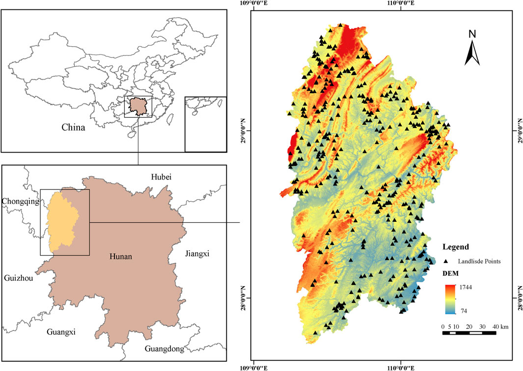
FIGURE 1. The study area and historical landslide hazard points.

2.2 Data sources

The information regarding landslide occurrences and geological lithology in Xiangxi Prefecture was collected from the Xiangxi Guoditong integrated spatial and temporal service platform. The data structure is in geographic vector format, including 402 landslide points and 356 geologic lithology units. The Digital Elevation Model (DEM) data were obtained from “ASTERGDEM DEM 30 m resolution digital elevation data” (https://search.earthdata.nasa.gov/search). NDVI data from “Landsat8OLI_TIRS Satellite Digital Product Data at 30 m Spatial Resolution” from the 2018 Geospatial Data Cloud (https://search.earthdata.nasa.gov/search). The annual precipitation data were acquired from “Global Precipitation Measurement Data level 3" (https://pmm.nasa.gov/precipitation -measurement-missions) of NASA for the year 2018, with annual precipitation. The unit is 1 mm, and the data with road, river and distance data with residential areas are from the first national geographic census re-sults data. For the convenience of statistics and analysis, combined with the resolution of DEM and remote sensing image data, The study area in Xiangxi Prefecture was par-titioned based on a raster resolution of 30 m × 30 m with a total of 31,374,840 raster units.

2.3 Trigger factors

The reasons behind landslide disasters are complex. The influencing factors are mainly divided into two classes: internal pregnancy factor (terrain landform, geological structure, transportation water system, etc.) and external induced factors (rainfall, earthquake, human engineering activities, etc.). LinJeng-Wen et al. analyzed the correlation between the factors, and the study’s results proved that the distinguishing factors are independent and can be used as factor variables (Li et al., 2022). This paper chooses 9 factors related to landslide disasters, including DEM, slope, aspect, lithology, distance to faults, distance to roads, rainfall, distance to rivers, and normalized difference vegetation index (NDVI), as illustrated in Supplementary Table S1 and Figure 2. The selection of these factors was based on the reliability of model prediction and the ease of calculating the three-dimensional convolution.

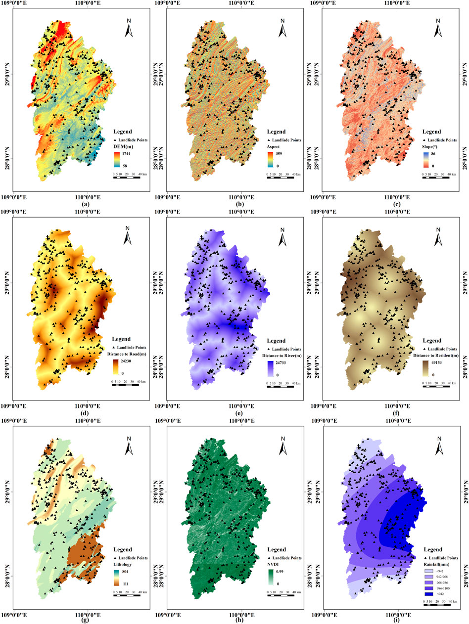
FIGURE 2. Diagrams of the landslide triggering factors.

3 Methodology

Figure 3 illustrates the method flowchart used for LSM in this study. First, this paper prepared landslide point data and landslide trigger factors to construct training and validation sets. Second, the SVMmodels were trained using 2D data format while the CNN and 3DCNN was trained using 3D data format. Then, the ROC curves were used for quantitative evaluation of the prediction results obtained by the three methods. Finally, the landslide susceptibility mapping is carried out with three trained models.

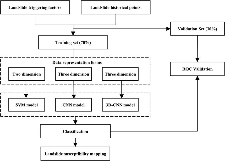
FIGURE 3. Flowchart of the present study.

3.1 SVM model

The SVM model is a binary classifier based on statistical learning theory that finds the maximum margin hyperplane. This model is effective in addressing various classification problems (Cherkassky and Yunqian, 2004). In the study of LSM, the j-th trigger factor of the i-th position in the layer is expressed as v_ij, i∈{1,2…,n}, j∈{1,2…,9}. Among them, the variable n represents the total number of samples, while j represents the number of categories of the landslide trigger factors. Then, the SVM model maps the input vector v into u and classifies it, using a non-linear mapping ϕ(v), to a high-dimensional feature space. as shown in Eq. 1.

The regression function of SVM, denoted by f(v), can be expressed as the inner product of a weight vector w and the input vector v, plus a bias term b. Alternatively, the optimization problem can be formulated with Lagrangian transformation and optimality constraints, allowing for the use of Eq. 2 to obtain f(x) (Cremmer et al., 1983).

where α_i and α_i* are the Lagrange multipliers, K (v, v_i) is a kernel function. This article uses the RBF kernel (Bugmann, 1998).

3.2 CNN model

The CNN model requires two-dimensional images as input, and the slope-unit or landslide unit is not suitable for cooperation as the input of the CNN model (as shown in Figure 4 left part). In order to solve this problem, the original data needs to be reconstructed. As shown in Figure 4 right part, the proposed method expands outward from the centre of the landslide slope unit in each layer of the landslide trigger factors layer to obtain the spatial characteristics of the sample data (Li and Lan, 2020). After that, the multi-layer grid data is brought into the CNN model for training.

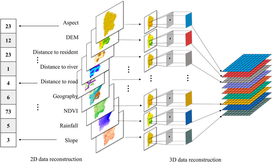
FIGURE 4. Reconstruction of two-dimensional input data.

In the convolutional layers, the CNN model runs a 2D convolution kernel that collects features from a nearby neighborhood on feature maps from the previous layer. The result is then passed through a sigmoid function with an additive bias. The value of the unit at position (x, y) in the jth feature map in the ith layer is denoted as v_ij^xy and can be expressed as follows:

the expression for v_ij^xy, the value of the unit at position (x, y) in the jth feature map in the ith layer in the CNN model, is given by the hyperbolic tangent function tanh (), where b_ij is the bias for this feature map, m indexes over the set of feature maps in the (i-1)th layer connected to the current feature map, w_ijk^pq is the value at the position (p, q) of the kernel connected to the kth feature map, and Q_i and P_i are the width and height of the kernel, respectively.

The subsampling layers reduce the feature map resolution by pooling over the local neighbourhood in the previous layer, which increases the invariance to input distortions. To construct the CNN architecture, multiple convolution layers and subsampling are stacked alternately. The CNN parameters, including the bias b_ij and the kernel weight w, are typically trained using supervised or unsupervised approaches. The backpropagation algorithm is employed to optimize all parameters in the CNN layer, with the objective of minimizing the loss function (LeCun et al., 1998). The formula is defined as follows:

The CNN model architecture, as shown in Figure 5, involves optimizing all parameters in the CNN layer using the backpropagation algorithm and minimizing the loss function, where the two variables l_i and l_i’ represent the actual label and tag of the i-th input sample, respectively. The parameters are updated iteratively until the loss value reaches convergence.

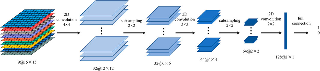
FIGURE 5. The structure of the CNN model.

3.3 3DCNN model

The CNN model applies 2D convolution kernels solely to the 2D feature maps, enabling the computation of features solely from the spatial dimensions of the single channel. Convolutional stages of CNNs must perform 3D data augmentation in order to simultaneously capture important features contained in several contiguous layers of 3D feature data. By convolving a 3D kernel into the cube created by stacking several trigger factors together, this method computes features from both the spatial and trigger factor dimensions. As a result of their connections to various trigger factors in the former layer, the feature maps in the cnn model are able to capture the pertinent features between landslide trigger factors. The value of the unit at position (x, y, z) on the j-th feature map in the i-th layer can be expressed as follows:

where R_i is the size of the 3D kernel along the landslide trigger factors dimension w_ijm^pqr and is the (p, q, r)-th value connected to the m-th feature map in the previous layer. Here, the value at position (x, y, z) on the jth feature map in the ith layer is determined by the (p, q, r)-th value connected to the m-th feature map in the previous layer, represented by w_ijm^pqr. The size of the 3D kernel along the landslide trigger factors dimension is denoted by R_i. Figure 6 depicts the architecture of the 3D convolutional kernel neural network.

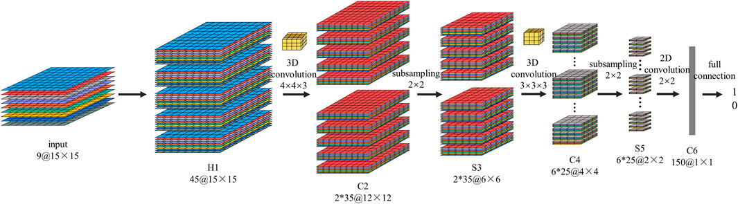
FIGURE 6. The architecture of the 3D augmented convolution kernel neural network.

The 3D cube that was recreated using the technique in Figure 4 is also used as input data for the 3DCNN model in the architecture depicted in Figure 6. We initially use a set of hardwired kernels to generate various information channels from the input frame, like H1 in Figure 6, in order to improve the feature amount in the vertical direction. The four directional Prewitt operators used by the feature hardwired kernel provide 45 feature maps in the second layer that are divided into five separate channels known as raw, horizontal gradient, vertical gradient, and two diagonal gradients. The attribute values of the input frames from the nine landslide trigger factors are contained in the original channel. By calculating the gradients along the horizontal, vertical, and two diagonal gradients on the nine landslide hazard factors, respectively, through the Prewitt operator, the feature maps in the horizontal gradient, vertical gradient, and two diagonal gradient channels are generated. Our prior knowledge of the characteristics is encoded in this hardwired layer, and this method typically provides greater performance than random initialization (Ji et al., 2012).

Then, we independently perform 3D convolutions to each of the 5 channels with a kernel size of 4 × 4×3 (3 in the trigger factor dimension, 4 × 4 in the spatial dimension). Using two sets of various solutions at each site, the number of feature maps is increased, yielding two sets of extracted features in the C2 layer, each with 35 feature maps. There are 490 trainable parameters in this layer. Each of the feature maps in the C2 layer is subjected to 2 × 2 subsampling in the subsequent subsampling layer S3, resulting in the same amount of feature maps with lower spatial resolution. This layer contains 140 trainable parameters. Applying 3D convolution with a kernel size of 3 × 3×3 on each of the five channels in the two sets of feature maps individually yields the next convolution layer, C4. We perform three convolutions with various kernels at each position to increase the number of feature layers, resulting in six separate sets of feature maps in the C4 layer, each of which has 25 feature maps. There are 840 trainable parameters in this layer. Each feature map in the C4 layer is subjected to 2 × 2 subsampling to produce the same amount of feature maps with lower spatial resolution in the subsequent layer S5. This layer contains 300 trainable parameters. We only do convolution in the spatial dimension at this layer because the temporal dimension’s size is already quite tiny at this point. The size of the output feature maps is reduced to 1 × 1 due to the convolution kernel size 2 × 2. All of the 150 1×1-sized feature maps in the C6 layer is connected to all 150 feature maps in the S5 layer.

The five input frames have been transformed into a 150D feature vector that captures the motion information in the input frames using many layers of convolution and subsampling. The number of units in the output layer equals the number of actions. The 150 units in the C6 layer are all fully connected to each unit. In this design, the 150D feature vector is subjected to a linear classifier in order to classify actions. The number of trainable parameters at the output layer for an action recognition issue with two classes (one class is a landslide, and the other is non-landslide) is 300.

4 Experimental results

4.1 Factors analysis and models construction

Based on the study area’s actual circumstances and an examination of topography, geomorphology, stratigraphic lithology, geological structure, rainfall, surface water, and human variables influencing the occurrence of landslides (Lin et al., 2019), as shown in Supplementary Table S2 the selected landslide trigger factors were tested for multiple covariances by stepwise regression method (Jiping et al., 2022). The correlation between each characteristic factor was tested by tolerance and variance inflation factor (VIF) is shown in Supplementary Table S2 (Kalantar et al., 2019). The findings demonstrate that the identified landslide trigger parameters have a tolerance greater than 0.1, and the variance inflation factor is less than 10, which indicates that each trigger factor has a low degree of co-linearity and good independence.

To create the model’s architecture, 804 samples (402 positive and 402 negative) from the entire dataset were used. Using these samples, databases for the Xiangxi Prefecture were created based on the number and distribution of landslide points. Next they were randomly divided into validation groups, which made up 30% of the total, and training groups, which comprised 70% of the total. Finally, each model was tested using both the validation dataset and the complete dataset. The parameters for the CNN and 3DCNN models are randomly initialized, and they are trained via online error backpropagation. The learn-ing rate was set to 0.0005 for the Xiangxi dataset, batch size, dropout rate, and epoch were set to 32, 0.5, and 150 in order to find the ideal hyperparameter.

Also, the weights were updated using SGD as the optimizer, and mean square error (MSE) was chosen as the loss function. The activation function was set to Tanh. The PSO approach is used to identify the ideal parameters for the SVM model by the penalty coefficient C and the RBF kernel function gamma (Fathi and Montazer, 2013). Our tests were run on Windows 10, 64-bit, an Intel i7-10700K processor running at 3.8 GHz with eight cores, 32 GB of RAM, and an NVIDIA GeForce RTX 2060Ti GPU (8 GB).

4.2 Validation and comparison methods

The evaluation of the three models’ effects in this paper was undertaken using the “ReceiverOperatingCharacteristic” curve for validation (Park and Kim, 2019). It is the relationship between specificity and sensitivity; it s a g. The logic behind this is that if a test is non-diagnostic, it is just as likely to produce a true positive or a false positive. Specificity, actual positive rate, true positive rate, and false positive rate all rise along with diagnostic competence. The accuracy of the evaluation model is shown by the area under the ROC curve (Area Under Curve, AUC). The evaluation model’s prediction effect is stronger the closer the area value is near 1. The area value, on the other hand, has no application value when it equals 0.5. Figure 7 displays the ROC curves and AUC values for the two models.

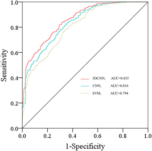
FIGURE 7. The ROC curve of three models with the 15 × 15 size of input data.

The 3DCNN model, CNN model, and SVM model all have AUC values of 0.835, 0.816, and 0.794, respectively, as shown in Figure 7. The three models may all have a higher prediction of LSM since the AUC regions of their ROC curves are all greater than 0.5. According to the specifics, the 3DCNN model’s ROC curve is situated in the upper-most left corner, which means that its AUC area is the largest and the point in the distance is farther from the reference line, indicating that the 3DCNN model is, in some ways, superior to the other two models. In other words, the 3DCNN of LSM model in Xiangxi Prefecture is more precise and reliable.

4.3 Landslide susceptibility mapping

To create the LSM for Xiangxi Tujia and Miao Autonomous Prefecture, this study used the SVM, CNN, and 3DCNN models (Figure 8). For the purpose of computing the landslide susceptibility index, all pixels within the study area were supplied into these trained models (LSI). The LSI was then separated into five susceptibility levels using ArcMap10.6’s natural break approach: very low (VLS), low (LS), moderate (MS), high (HS), and very high (VHS). The landslide susceptibility zones, which show the proportion of each susceptibility level to the entire study region, were employed to qualitatively examine the LSM.

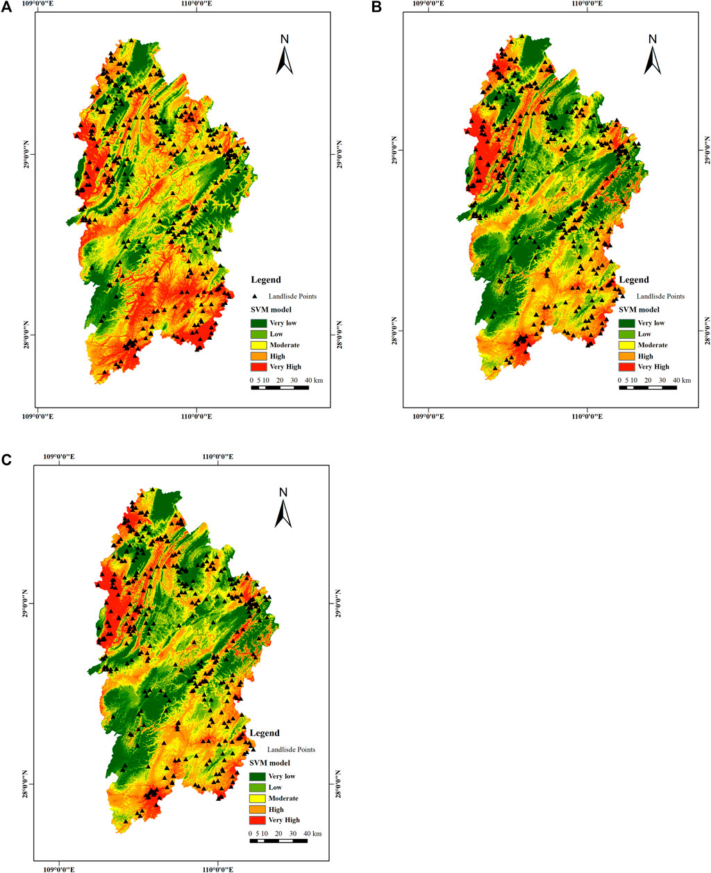
FIGURE 8. Evaluation results of landslide susceptibility mapping. (A) LSM of the SVM model; (B) LSM of the CNN model; (C) LSM of the 3DCNN model.

As shown in Figure 8, the VHS zones are mostly found in Xiangxi Prefecture’s southeast and northwest. Due to the long gullies, steep slopes, complex geological structures, and two major rivers running through the area, coupled with the increasing human engineering activities (such as road projects), the area is highly susceptible to landslide disasters.

The analysis and counting of non-landslide and landslide hazard points in the training samples was done using ArcMap. After that, we determine what percentages of landslide points and non-landslide points are located in each of the five prone zones.

Supplementary Table S3 shows that the majority of landslide hazard spots are anticipated to have high and extremely high susceptibility zones. A relative association between historical landslide events and susceptibility areas is demonstrated by the fact that few landslides occur in places with relatively low susceptibility. Furthermore, more than 80% of historical landslide events for all methods were located in high-sensitivity areas, confirming the plausibility of landslide susceptibility mapping. The percentage of hazard points in each zone likewise gradually grew according to the 3DCNN, CNN, and SVM models. The highest percentages were 47.51%, 39.30%, and 30.85% in the high-prone area. Hence, the proportion of the number of disaster points is more significant than that of other districts, and the proportions are 47.51%, 39.30%, and 35.57%. We found that all three model methods can predict the susceptibility of landslide hazards very well. Compared with the CNN and SVM models, the 3DCNN model has higher accuracy.

4.4 Scale size and model performance

In order to research how the spatial scale of the data input affects the LSM using the 3DCNN model, we compared the input data structures at five different spatial scales of 9 × 9, 15 × 15, 21 × 21, 27 × 27, 33 × 33, and 39 × 39. Furthermore, we compared and analyzed the ROC curve of the corresponding 3DCNN model. In Figure 9, the experimental outcomes are displayed. The 3D CNN model’s ROC curve varies depending on the input data scales. As the spatial scale increases, the AUC value of 3DCNN gradually increases. When the sample point range is expanded to 21 × 21, the AUC value reaches the maximum value of 0.859. The AUC value rapidly declines, reaching a minimum of 0.781, which is 0.078 lower than the highest AUC value and even worse than the performance of the CNN model and the SVM model, as the sample space size rises to 39 × 39. The above reasoning proves that scale does affect LSM performance, but this effect varies with size. A further comparative study of the relationship between area and scale in the landslide samples found that the average length and width of the landslide samples in Xiangxi Prefecture used in this paper are 281.5 m and 563.7 m, respectively, projected to a grid of 10 × 20 landslide units (Supplementary Table S4).

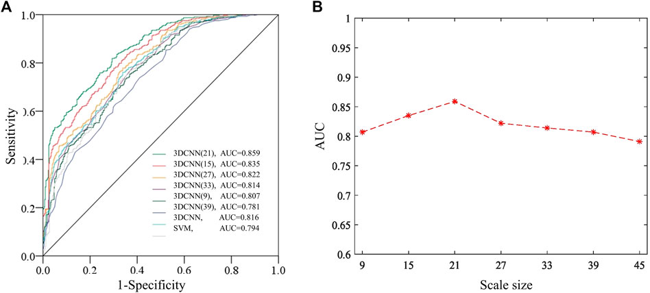
FIGURE 9. The ROC curve. (A) The ROC curve with different scale sizes of input data; (B) The 3DCNN model’s AUC and input data’s spatial resolution connection.

5 Discussions

LSM is essential for creating a thematic map that shows where and how likely landslides are to occur. A landslide list made up of landslide points and the association between landslide trigger variables is the basis of LSM. Landslides, as a regional geographic entity, are considered incomplete only in terms of points, with no spatial characteristics or correlation feature between the landslide trigger factors. This research aims to convert point landslide data into three-dimensional data by incorporating spatial and correlation features between landslide trigger factors. To do this, the fundamental module that we deployed was a convolutional neural network. In order to allow for synergy, we suggested a 3DCNN model that incorporates spatial and fators correlation features among landslide trigger components.

By reducing variation and bias in prior related studies, the hybrid model was considered to improve the ability to forecast land slides. In our tests, the proposed 3DCNN model performed better in terms of AUC than the other examined models. These results met the hybrid model’s expectations to some extent and can be considered promising. Meanwhile, the CNN-based models outperformed conventional machine learning models regarding overall performance (SVM). This is because the intricate design of CNN-based models enhances their capacity to collect representations of landslides at deep levels through convolution and pooling procedures.

Aside from that, the suggested 3DCNN technique beat the other two CNN-based models, as shown in Figure 8 and Figure 9. This makes sense because by extracting geographical data and correlation features between landslide trigger components from the land-slide inventory, the 3DCNN model improved landslide prediction accuracy. Using the suggested 3DCNN model, more representations linked to landslides were recovered from the limited datasets.

The contradiction between the complex structure and the scale landslide samples necessitates avoiding overfitting despite CNN’s outstanding feature extraction capabilities. We plot ROC curves on training sets with varying scale sizes to further validate the models’ fit. According to Figure 9 and Supplementary Table S4, 3DCNN has the maximum AUC value at a scale of 21 × 21, with a value of 0.859. The ROC curves also vary depending on the geographic scale of the data input. The model’s predictive performance gradually declines as the spatial scale increases. When the size of the input data unit was compared to the actual length and width of the landslide (Supplementary Table S4), we discovered that the landslide is a regional target with a limited spatial scale. Other noise effects are amplified as the spatial scale is increased indefinitely. As a result, the model’s accuracy in predicting landslide risk will decrease after reaching the maximum spatial characteristic gain. To summarise, the CNN landslide susceptibility model combined with spatial features should consider the sample’s spatial scale.

The susceptibility maps can also show how plausible and reliable the models are. Figure 8 illustrates how the majority of landslides in the 3DCNN models occurred in the LSM’s VH susceptibility zone. This indicates that the constructed models can accurately determine the likelihood of a landslide occurring and provide acceptable hazard mitigation methods to decision-makers, which is good news from the perspective of disaster mitigation. Additionally, scientists evaluate a susceptibility model’s dependability using the Specificity and Sensitivity indices. By correctly categorizing non-landslide zones as stable slopes and maximizing land usage, highly accurate models can avoid financial losses. By precisely identifying landslide-prone locations, high-sensitivity value models can also offer safe mitigating advice. The suggested model in the current study outperformed other baseline models in the validation set in terms of specificity and sensitivity, highlighting the dependability of disaster mitigation and land use planning.

6 Conclusion

We conducted our research in the Hunan Province’s Xiangxi Prefecture for this paper. Experiments show that the relationship between disaster-causing factors and spatial characteristics affects the LSM prediction model’s accuracy. Under the same conditions as the SVM and CNN models, increasing the spatial characteristics of landslide hazard factors can improve LSM prediction accuracy. However, due to the model’s complexity, the sample space scale limits this accuracy. The experimental results confirmed this hypothesis as well. The model performs best when the sample point range is expanded to 21 regions, i.e., when the input sample size covers the actual area of the landslide. Because the sample LSM based on points ignores the objective spatial attributes, expanding the factor or expanding the sample area can improve the LSM’s prediction accuracy. However, due to data constraints, this paper only considers the impact of a scale change in 30 m resolution sample data on LSM prediction accuracy. It does not consider landslide hazard factors in different resolution scenarios, even if the optimal scale value varies. We intend to investigate this step further in our subsequent paper.

Data availability statement

The original contributions presented in the study are included in the article/Supplementary Material, further inquiries can be directed to the corresponding author.

Author contributions

CC, SB, and JD made a considerable contribution to the writing, design, data gathering, statistical analysis, and experimental planning. JL, SX, and JD all made major contributions to the interpretation of data and the intellectual revision of the text. All writers reviewed and approved the final version. The manuscript has been published with the consent of all authors who have read and approved it.

Funding

This research was funded by the National Key Research and Development Program of China (2022YFC3005705 and 2020YFC1511704).

Conflict of interest

The authors declare that the research was conducted in the absence of any commercial or financial relationships that could be construed as a potential conflict of interest.

Publisher’s note

All claims expressed in this article are solely those of the authors and do not necessarily represent those of their affiliated organizations, or those of the publisher, the editors and the reviewers. Any product that may be evaluated in this article, or claim that may be made by its manufacturer, is not guaranteed or endorsed by the publisher.

Supplementary material

The Supplementary Material for this article can be found online at: https://www.frontiersin.org/articles/10.3389/fenvs.2023.1177891/full#supplementary-material

References

Balogun, A.-L., Rezaie, F., Pham, Q. B., Gigović, L., Drobnjak, S., Aina, Y. A., et al. (2021). Spatial prediction of landslide susceptibility in western Serbia using hybrid support vector regression (SVR) with GWO, BAT and COA algorithms. Geosci. Front. 12 (3), 101104. doi:10.1016/j.gsf.2020.10.009
Bragagnolo, L., da Silva, R. V., and Grzybowski, J. M. V. (2020). Artificial neural network ensembles applied to the mapping of landslide susceptibility. Catena 184, 104240. doi:10.1016/j.catena.2019.104240
Bugmann, G. (1998). Normalized Gaussian radial basis function networks. Neurocomputing 20 (1–3), 97–110. doi:10.1016/s0925-2312(98)00027-7
Cherkassky, V., and Yunqian, M. (2004). Practical selection of SVM parameters and noise estimation for SVM regression. Neural Netw. 17 (1), 113–126. doi:10.1016/S0893-6080(03)00169-2
Cremmer, E., Ferrara, S., Girardello, L., and Van Proeyen, A. (1983). Yang-mills theories with local supersymmetry: Lagrangian, transformation laws and super-Higgs effect. Nucl. Phys. B 212 (3), 413–442. doi:10.1016/0550-3213(83)90679-X
Fathi, V., and Montazer, G. A. (2013). An improvement in RBF learning algorithm based on PSO for real time applications. Neurocomputing 111, 169–176. doi:10.1016/j.neucom.2012.12.024
Fauvel, M., Tarabalka, Y., Benediktsson, J. A., Chanussot, J., and Tilton, J. C. (2013). Advances in spectral-spatial classification of hyperspectral images. Proc. IEEE 101 (3), 652–675. doi:10.1109/jproc.2012.2197589
Gao, Z., and Ding, M. (2022). Application of convolutional neural network fused with machine learning modeling framework for geospatial comparative analysis of landslide susceptibility. Nat. Hazards 113, 833–858. doi:10.1007/s11069-022-05326-7
Ghamisi, P., Dalla Mura, M., and Benediktsson, J. A. (2015). A survey on spectral spatial classification techniques based on attribute profiles. IEEE Trans. Geoscience Remote Sens. 53 (5), 2335–2353. doi:10.1109/tgrs.2014.2358934
Ghorbanzadeh, O., Blaschke, T., Gholamnia, K., Raj Meena, S., Tiede, D., and Aryal, J. (2019). Evaluation of different machine learning methods and deep-learning convolutional neural networks for landslide detection. Remote Sens. 11 (2), 196. doi:10.3390/rs11020196
Hong, H., Pradhan, B., Sameen, M. I., Kalantar, B., Zhu, A., and Chen, W. (2017). Improving the accuracy of landslide susceptibility model using a novel region-partitioning approach. Landslides 15 (4), 753–772. doi:10.1007/s10346-017-0906-8
Huang, F., Yan, J., Fan, X., Yao, C., Huang, J., Chen, W., et al. (2022). Uncertainty pattern in landslide susceptibility prediction modelling: Effects of different landslide boundaries and spatial shape expressions. Geosci. Front. 13 (2), 101317. doi:10.1016/j.gsf.2021.101317
Ji, S., Xu, W., Yang, M., and Yu, K. (2012). 3D convolutional neural networks for human action recognition. IEEE Trans. Pattern Analysis Mach. Intell. 35 (1), 221–231. doi:10.1109/TPAMI.2012.59
Jiping, L., Enjie, L., Shenghua, X. U., Mengmeng, L., Wang, Y., Zhang, F., et al. (2022). Multi-kernel support vector machine considering sample optimization selection for analysis and evaluation of landslide disaster susceptibility. Acta Geod. Cartogr. Sinica 51 (10), 2034. doi:10.11947/j.AGCS.2022.20220326
Kalantar, B., Ueda, N., Lay, U. S., Al-Najjar, A. H. H., and Halin, A. A. (2019). “Conditioning factors determination for landslide susceptibility mapping using support vector machine learning,” in IGARSS 2019 - 2019 IEEE International Geoscience and Remote Sensing Symposium, Yokohama, Japan, 28 July 2019 - 02 August 2019, 9626–9629. doi:10.1109/IGARSS.2019.8898340
LeCun, Y., Bottou, L., Bengio, Y., and Haffner, P. (1998). Gradient-based learning applied to document recognition. Proc. IEEE 86 (11), 2278–2324. doi:10.1109/5.726791
Li, L., and Lan, H. (2020). Integration of spatial probability and size in slope-unit-based landslide susceptibility assessment: A case study. Int. J. Environ. Res. Public Health 17 (21), 8055. doi:10.3390/ijerph17218055
Li, W., Chen, H., Liu, Q., Liu, H., Wang, Y., and Gui, G. (2022). Attention mechanism and depthwise separable convolution aided 3DCNN for hyperspectral remote sensing image classification. Remote Sens. 14 (9), 2215. doi:10.3390/rs14092215
Li, Y., Zhang, H., and Shen, Q. (2017). Spectral–spatial classification of hyperspectral imagery with 3D convolutional neural network. Remote Sens. 9 (1), 67. doi:10.3390/rs9010067
Lin, J.-W., Hsieh, M.-H., and Li, Y.-J. (2019). Factor analysis for the statistical modeling of earthquake-induced landslides. Front. Struct. Civ. Eng. 14 (1), 123–126. doi:10.1007/s11709-019-0582-y
Liu, J., and Liang, E. (2022). Evaluation of landslide disaster susceptibility in multi-core SVM based on sample selection strategy. Geomatics Inf. Sci. Wuhan Univ. 51 (10), 2034–2045.
Liu, R., Yang, X., Xu, C., Wei, L., and Zeng, X. (2022). Comparative study of convolutional neural network and conventional machine learning methods for landslide susceptibility mapping. Remote Sens. 14 (2), 321. doi:10.3390/rs14020321
Liu., K. (2020). Earthquake-induced failure mechanism and stability evalution of loess slope under rainfall effects. Lanzhou: Lanzhou University. doi:10.27204/d.cnki.glzhu.2020.001256
Luo, L., Xiangjun, P., Huang, R., Zuan, P., and Ling, Z. (2021). Landslide susceptibility assessment in jiuzhaigou scenic area with GIS based on certainty factor and logistic regression model. J. Eng. Geol. 29 (2), 526–535.
Ministry of Natural Resources of the People’s Republic of China (2021). National geological hazard disaster situation in 2021 and geological hazard trend prediction in 2022. Beijing: Ministry of Natural Resources of the People’s Republic of China.
Nhu, V. H., Shirzadi, A., Shahabi, H., Singh, S. K., Al-Ansari, N., Clague, J. J., et al. (2020). Shallow landslide susceptibility mapping: A comparison between logistic model tree, logistic regression, naive bayes tree, artificial neural network, and support vector machine algorithms. Int. J. Environ. Res. Public Health 17 (8), 2749. doi:10.3390/ijerph17082749
Park, S., and Kim, J. (2019). Landslide susceptibility mapping based on random forest and boosted regression tree models, and a comparison of their performance. Appl. Sci. 9 (5), 942. doi:10.3390/app9050942
Plaza, A., Martinez, P., Perez, R., and Plaza, J. (2004). A new approach to mixed pixel classification of hyperspectral imagery based on extended morphological profiles. Pattern Recognit. 37 (6), 1097–1116. doi:10.1016/j.patcog.2004.01.006
Sajadi, P., Sang, Y.-F., Gholamnia, M., Bonafoni, S., and Mukherjee, S. (2022). Evaluation of the landslide susceptibility and its spatial difference in the whole qinghai-Tibetan plateau region by five learning algorithms. Geosci. Lett. 9 (1), 9. doi:10.1186/s40562-022-00218-x
Shi, C., and Pun, C. M. (2017). Superpixel-based 3D deep neural networks for hyperspectral image classification. S0031320317303515. Chicago, U.S.A.: Pattern Recognition.
Sun, D., Xu, J., Wen, H., and Wang, D. (2021). Assessment of landslide susceptibility mapping based on bayesian hyperparameter optimization: A comparison between logistic regression and random forest. Eng. Geol. 281, 105972. doi:10.1016/j.enggeo.2020.105972
Tobler, W. R. (1970). A computer movie simulating urban growth in the detroit region. Econ. Geogr. 46, 234–240. doi:10.2307/143141
Wang, Q., Wang, Y., Niu, R., and Peng, L. (2017). Integration of information theory, K-means cluster analysis and the logistic regression model for landslide susceptibility mapping in the three gorges area, China. Remote Sens. 9 (9), 938. doi:10.3390/rs9090938
Wang, Y., Fang, Z., and Hong, H. (2019). Comparison of convolutional neural networks for landslide susceptibility mapping in yanshan county, China. Sci. Total Environ. 666, 975–993. doi:10.1016/j.scitotenv.2019.02.263
Wei, R., Ye, C., Ge, Y., and Yao, L. (2022a). An attention-constrained neural network with overall cognition for landslide spatial prediction. Landslides 19 (5), 1087–1099. doi:10.1007/s10346-021-01841-z
Wei, R., Ye, C., Sui, T., Ge, Y., Yao, L., and Li, J. (2022b). Combining spatial response features and machine learning classifiers for landslide susceptibility mapping. Int. J. Appl. Earth Observation Geoinformation 107, 102681. doi:10.1016/j.jag.2022.102681
Wu, X., Chen, X., Benjamin Zhan, F., and Song, H. (2015). Global research trends in landslides during 1991–2014: A bibliometric analysis. Landslides 12 (6), 1215–1226. doi:10.1007/s10346-015-0624-z
Xu, S., Liu, J., Wang, X., Zhang, Y., Lin, R., Zhang, M., et al. (2020). Landslide susceptibility assessment method incorporating index of entropy based on support vector machine: A case study of shaanxi Province. J. Wuhan Univ. Inf. Sci. Ed. 45 (8), 1214–1222.
Yang, Z., Xu, C., Shao, X., Ma, S., and Li, L. (2022). Landslide susceptibility mapping based on CNN-3D algorithm with attention module embedded. Bull. Eng. Geol. Environ. 81 (10), 412. doi:10.1007/s10064-022-02889-4
Zhao, Z., Liu, Z. Y., and Xu, C. (2021). Slope unit-based landslide susceptibility mapping using certainty factor, support vector machine, random forest, CF-SVM and CF-rf models. Front. Earth Sci. 9, 589630. doi:10.3389/feart.2021.589630
Zhu, A.-X., Miao, Y., Liu, J., Bai, S., Zeng, C., Ma, T., et al. (2019). A similarity-based approach to sampling absence data for landslide susceptibility mapping using data-driven methods. Catena 183, 104188. doi:10.1016/j.catena.2019.104188
Keywords: 3DCNN, spatial-factor features, landslide susceptibility, trigger factos, scale comparison
Citation: Liu M, Liu J, Xu S, Chen C, Bao S, Wang Z and Du J (2023) 3DCNN landslide susceptibility considering spatial-factor features. Front. Environ. Sci. 11:1177891. doi: 10.3389/fenvs.2023.1177891
Received: 02 March 2023; Accepted: 14 April 2023;
Published: 21 April 2023.
Edited by:
Long Yan, Central South University, ChinaReviewed by:
Yahui Guo, Beijing Normal University, ChinaJoao Paulo Moura, University of Trás-os-Montes and Alto Douro, Portugal
Copyright © 2023 Liu, Liu, Xu, Chen, Bao, Wang and Du. This is an open-access article distributed under the terms of the Creative Commons Attribution License (CC BY). The use, distribution or reproduction in other forums is permitted, provided the original author(s) and the copyright owner(s) are credited and that the original publication in this journal is cited, in accordance with accepted academic practice. No use, distribution or reproduction is permitted which does not comply with these terms.
*Correspondence: Jiping Liu, liujp@casm.ac.cn