A Test of Species Distribution Model Transferability Across Environmental and Geographic Space for 108 Western North American Tree Species

Introduction

Unprecedented environmental change caused by human activity threatens biodiversity and its associated ecosystem functions and services that humanity relies upon (Chapin et al., 2000; Scheffers et al., 2016). In this era of rapid global change, forecasts of biodiversity changes have the potential to inform conservation decisions to minimize extinctions (Botkin et al., 2007). Species distribution models (SDMs) are one of the most accessible tools for spatial predictions of biodiversity at biogeographic extents and various open-source software packages are available for SDM implementation (Brown, 2014; Thuiller, 2014; Kass et al., 2018). Part of the popularity of correlative SDMs lies in the increasing availability of data needed to fit them (i.e., species occurrence records and satellite remotely sensed environmental data; Turner, 2014; Record and Charney, 2016). In addition, process-based data on species’ demography, dispersal, biotic interactions, and other data needed for fitting mechanistic SDMs is often lacking, especially across the entirety of a species range (e.g., for process-based demographic distribution models (Evans et al., 2016; Kindsvater et al., 2018) or range wide models incorporating biotic interactions (Zarnetske et al., 2012; Belmaker et al., 2015). Despite the limitations of SDMs (Pearson and Dawson, 2003; Belmaker et al., 2015), they remain a common and useful tool for predicting potential changes in species distributions and suitable habitat (Record et al., 2018). Understanding the limitations of SDMs is thus necessary to inform their appropriate use.

Studies typically assume that correlative SDMs capture some aspect of a species’ niche which can be generalized to other times or locations (Anderson, 2013). This assumption is known as model transferability — the ability of a model to generate precise and accurate predictions for a new set of observations (i.e., in space or time) that were not used in fitting the model (Yates et al., 2018). Transferability of SDMs is typically assessed with three types of ‘validation’ data (reviewed by Bahn and McGill, 2013; Werkowska et al., 2017; Sequeira et al., 2018; Yates et al., 2018): (1) independently collected data (e.g., Elith et al., 2006), (2) temporally independent data (e.g., Record et al., 2013), and (3) spatially independent data (e.g., Randin et al., 2006).

Studies assessing SDM transferability across taxa and geographic locations have shown inconsistent results — some SDMs transfer well, and others do not (reviewed by Sequeira et al., 2018; Yates et al., 2018). For instance, Duncan et al. (2009) investigated five South African dung beetle species to see if their native ranges could predict their invasive ranges in Australia and found that this approach worked well for two of the species, but not for the other three. Using a similar approach that leveraged native and invasive distribution data, Ibáñez et al. (2009) found that spatially explicit hierarchical Bayesian SDMs parameterized with data from both the native and invasive geographic ranges of three woody plants generated better predictions of the presence/absence of them in their invasive range than models fitted with data only from their native geographic range. This result suggested that the niches of these species may be better captured by incorporating information from the native and invasive geographic ranges of these invasive species. Whereas Duncan et al. (2009) and Ibáñez et al. (2009) illustrate some instances where SDMs transfer in geographic space, other studies illustrate poor transferability of SDMs. For instance, a study of the presence and absence of 54 alpine and subalpine plants on the ability of SDMs to transfer in geographic space between Switzerland and Australia found that overall transferability was poor (Randin et al., 2006). A cross-time study from tropical montane cloud forests showed that extrapolation in environmental space in the present led to poor transferability when predicting the past (Guevara et al., 2018). A study of mammals from North America and Australia found that Maxent models did not transfer well when training and testing data from different geographic regions were dissimilar in their environmental conditions, resulting in collinearity shifts between training and testing environmental predictor variables (Feng et al., 2019). These inconsistent results suggest that there are theoretical and technical knowledge gaps inhibiting effective SDM transferability.

To improve SDM transferability a recent review by 50 experts identified fundamental and technical knowledge gaps that need to be addressed (Yates et al., 2018). One of the fundamental knowledge gaps was determining the limits to extrapolation (spatial and/or temporal) in model transfers. A focus on spatial limits to extrapolation is especially promising because spatially independent data provide the best test of SDM transferability (Bahn and McGill, 2013). Further, independently collected data may introduce noise due to differences in methodology and still does not affirm that the data are spatially independent (Elith et al., 2006). In addition, temporally independent data sets do not guarantee that there is no temporal autocorrelation between data used for model fitting and data used for model validation (Bahn and McGill, 2013).

Assessments of transferability in space often take three approaches:

(i) Holdout geographic transferability involves testing models fit in different locations but within the same portion of environmental space (e.g., as measured by a convex hull in environmental space). For instance, one might test transferability within the same geographic region, in which case training and testing plots may be relatively near one another. In such cases, similar mechanisms underlying spatial autocorrelation may persist in both testing and training data, and hence one has more confidence that the same ecological processes are relevant in both the training and testing data (Record et al., 2013; Sillero and Barbosa, 2020).

(ii) Novel geographic transferability involves testing transferability to a different geographic region, in which case training and testing plots are considerably more spatially distant. Such tests are useful to remove patterns of spatial autocorrelation between training and testing data, however rather different processes may constrain occurrence patterns in different regions (e.g., different types of disturbance; (Dirnböck et al., 2003; McAlpine et al., 2008) and the potential for extrapolation to different processes is greater.

(iii) Environmental transferability requires extrapolation in environmental space, which may be in the same or a different geographic region from the training data. Tests of environmental transferability are useful in evaluating the generality of the fitted response curves (i.e., occurrence-environment relationships) to characterize a species niche but the niche may be considerably truncated in the fitting region (Thuiller et al., 2004). A truncated niche may lead to response curves that are inappropriate for extrapolation (e.g., one side of a unimodal response, when truncated, appears to be monotonic, which will extrapolate poorly; Hannemann et al., 2016).

In addition to determining limits to spatial extrapolation, Yates et al. (2018) also identified a knowledge gap in determining how model complexity influences transferability as an impediment to confidence in transferring SDMs. Model complexity may refer to the number of explanatory variables (i.e., dimensionality; Peterson, 2011), transformations of those explanatory variables (i.e., ‘features’ with regards to machine learning) and/or the intricacies of the algorithm that characterizes the shape of the occurrence-environment relationships and is tightly linked to the number of parameters in the model (Werkowska et al., 2017; Brun et al., 2020). As with any modeling, in the spirit of generality, simpler SDMs are preferred over complex models (i.e., Occam’s Razor; Young et al., 2010).

Merow et al. (2014) reviewed algorithm complexity in SDMs to ask how much intricacy is needed for optimal extrapolation. They found that simpler parametric models (e.g., generalized linear models) may miss thresholds that distinguish presence from absence locations in relation to the environment, whereas more complex non-parametric models (e.g., generalized additive models) may extrapolate poorly when the response curve forms odd shapes at the edge of the observed data range if there are few points there. In a similar vein, they also found that machine learning models that use a flat response beyond the observed data range (i.e., clamping) tend to overestimate an organism’s environmental tolerance. How model complexity influences the ability of SDMs to transfer and extrapolate in space remains a fundamental knowledge gap that limits our confidence in SDMs for conservation applications (Yates et al., 2018).

To improve understanding of spatial limits to SDM extrapolation and to quantify how model complexity influences transferability, we assessed three types of transferability— holdout geographic transferability, novel geographic transferability, and environmental transferability—for 11 model algorithms of varying complexity. We used presence/absence data for 108 tree species from the United States Forest Service’s Forest Inventory and Analysis (FIA). These data serve as an optimal study system for tests of transferability due to the abundant presence and absence sampling across geographic and environmental space, which allows for explicit testing of factors affecting transferability and therefore results can be more aptly applied to other systems (Sequeira et al., 2018).

We addressed the following questions:

(1) How does transferability in geographic space (i.e., holdout geographic transferability vs. novel geographic transferability) depend upon SDM algorithms?

(2) What is the relationship between predictive performance of SDMs and amount of extrapolation in novel geographic space?

(3) What is the relationship between predictive performance of SDMs and amount of extrapolation in environmental space in a novel geographic region?

(4) Does the relationship between predictive performance of SDMs and amount of extrapolation in geographic and environmental space vary with SDM algorithms?

With regards to questions three and four, the intent of this study is to explore how models transfer in space when there are likely differences between the environmental conditions in training and testing regions as parts of our study region are likely to experience no-analog conditions (Williams and Jackson, 2007), thus we provide a stringent test of spatial transferability (Muscarella et al., 2014). We conclude with a discussion of alternative approaches to SDMs for situations when predictive performance declines at the spatial limits to SDM extrapolation, such as process-based models and approaches that focus on understanding distributions of geologically diverse areas rather than distributions of species.

Materials and Methods

Occurrence Data

The United States Forest Service’s (USFS) FIA National Program provides data on species presence/absence, abundance, and basal area in established plots for all individuals >12.7 cm diameter at breast height. Given that the goal of this study was to use the dense FIA data to understand how common uses of SDMs under the data limitations faced by most studies for which these types of climate envelope models are run (i.e., presence/absence or presence-only), we chose to model presence/absence rather than abundance or basal area. We downloaded all available FIA data within our study region with inventory years from 1950 to 2000 in the western United States (N 25.893–49.000°, W 124.799–97.175°; Figure 1), which included 286,551 census plot locations encompassing 254 species. Species were deemed present in a plot if they were observed anytime between 1950 and 2000 and were considered absent if otherwise. We recognize that generally it is not recommended to mix FIA plots for calculations of abundance (e.g., basal area) from different inventories prior to 2001 given that plot sizes varied from region to region depending on forest stand conditions before the United States Forest Service adopted a uniform nationwide sampling strategy (Gillespie, 1999; Bechtold and Peterson, 2005). However, we felt that using the 1950–2000 data was appropriate given that the data used for this study were presence/absence rather than abundance and the goal of this study was to explore SDM transferability for which studies from the literature are often comprised of presence-only observations (e.g., museum specimens) that lack any information on the amount of area searched for a given species. Furthermore, using the pre-2001 data in this study enabled us to increase the number of plots in the study region by an order of magnitude (i.e., from tens of thousands to hundreds of thousands of plots) to provide more information on species distributions throughout the western United States.

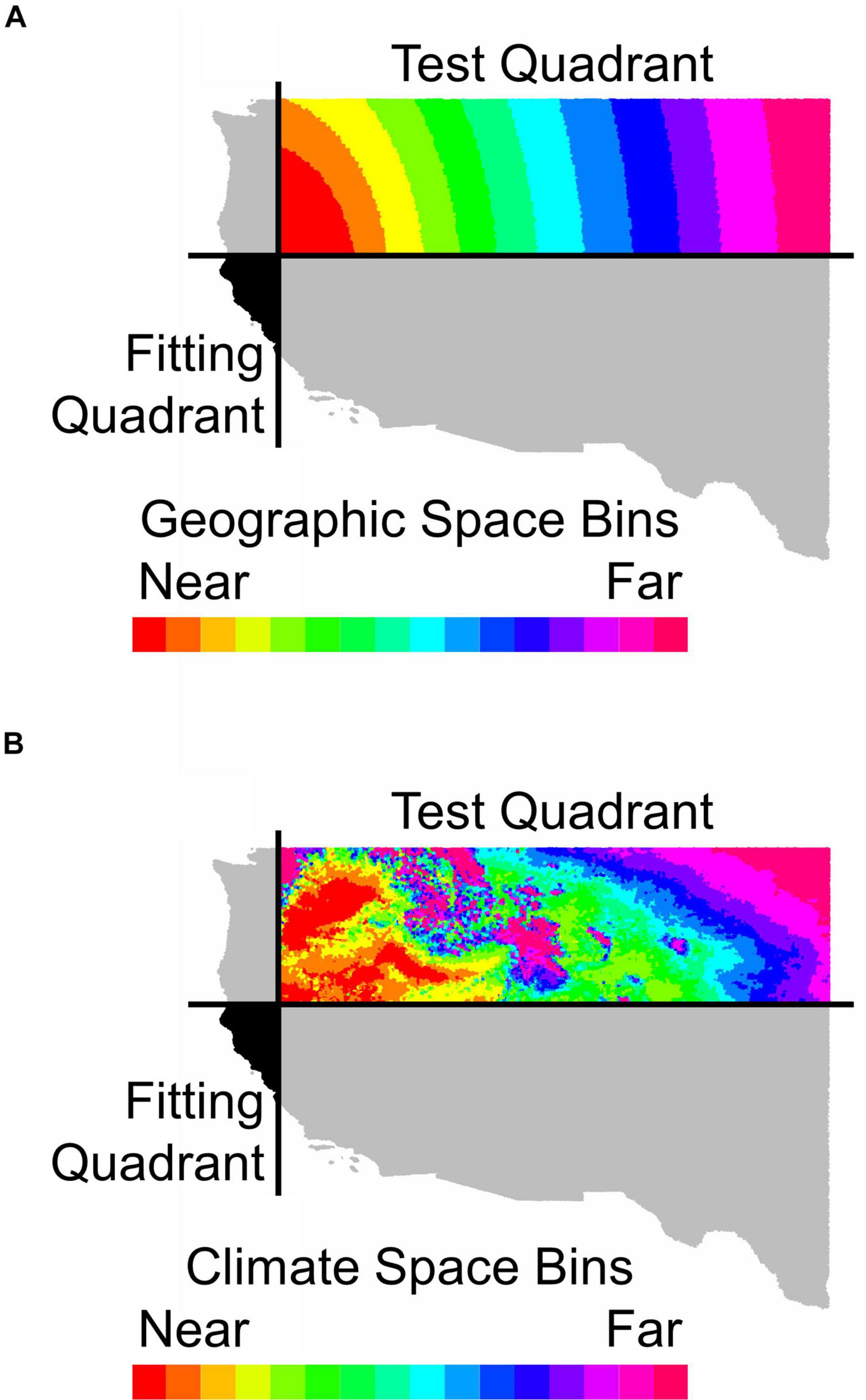
Figure 1. An illustration of how holdout sites were binned by distance (A) in geographic space or (B) in environmental space from the fitting region for Calocedrus decurrens. This map depicts the geographic extent of all FIA data used in the study. The horizontal and vertical black lines in (A,B) represent median latitude and longitude, respectively. The black area shows the quadrant used for model fitting and gray shaded quadrants were neither used for model fitting or testing. The colored areas indicate bins in either geographic or environmental space used for model testing with near and far referring to distance in geographic or climatic space.

Exact plot locations of FIA data are not publicly available due to legal concerns regarding privacy of landowners. The USFS ‘fuzzed’ and ‘swapped’ the exact plot locations of the data used in this study by masking the locations within a 500-acre area and exchanging plot coordinates for <10% of ecologically similar plots within the same county, respectively. In our analyses, we included only the 108 species with >120 presences (Supplementary Data Sheet 1).

Environmental Data

For fitting and predicting the models, we downloaded monthly climate data (i.e., precipitation and temperature) with a resolution of 30 arc seconds from the NASA Earth Exchange Downscaled Climate Predictions (NEX-DCP30¹) spanning the period from 1950 to 2000, which combines PRISM data from 1981 to 2000 and CMIP5 retrospective model runs to provide a long-term climatic average (Daly et al., 1994; Thrasher et al., 2013). We used the longer-term NEX-DCP30 historic climatic data for fitting models, as opposed to Worldclim historic climate from 1970 to 2000, because longer-term climatic averages provide better predictive power for long-lived species, such as trees (Lembrechts et al., 2019). For each year, we used the monthly data to generate 19 annual bioclimatic variables with the ‘biovars’ function from the dismo package in R (Hijmans et al., 2020). We averaged across all years from 1950 to 2000 to generate a single set of bioclimatic layers for model fitting and prediction. We did not include non-climatic predictor variables (e.g., elevation, soil, other physiographic variables) because many attempts to predict range size neglect non-climate factors, and this analysis was meant to compare only uses of that simplified approach.

Since some, but not all, of the models we used required uncorrelated predictor variables to meet model assumptions (e.g., GLM), we ran all models once with correlated variables and once excluding the minimum number of bioclimatic predictor variables with correlations ≥ | 0.7| (Dormann et al., 2013; Feng et al., 2019; Sillero and Barbosa, 2020; Supplementary Figure 1). This left nine bioclimatic variables for modeling: mean diurnal range (bio2), isothermality (bio3), maximum temperature of the warmest month (bio5), temperature annual range (bio7), mean temperature of the wettest quarter (bio8), mean temperature of the driest quarter (bio9), precipitation of the driest quarter (bio17), precipitation of the warmest quarter (bio18), and precipitation of the coldest quarter (bio19). Because we subdivided our data into quadrants for each species (Figures 1, 2), standardizing predictor variables across all four quadrants would have left each quadrant unstandardized independently, whereas standardizing the quadrants separately would have introduced differences between training and testing data. Therefore, to preserve our capacity to test transferability, we did not standardize predictor variables prior to fitting.

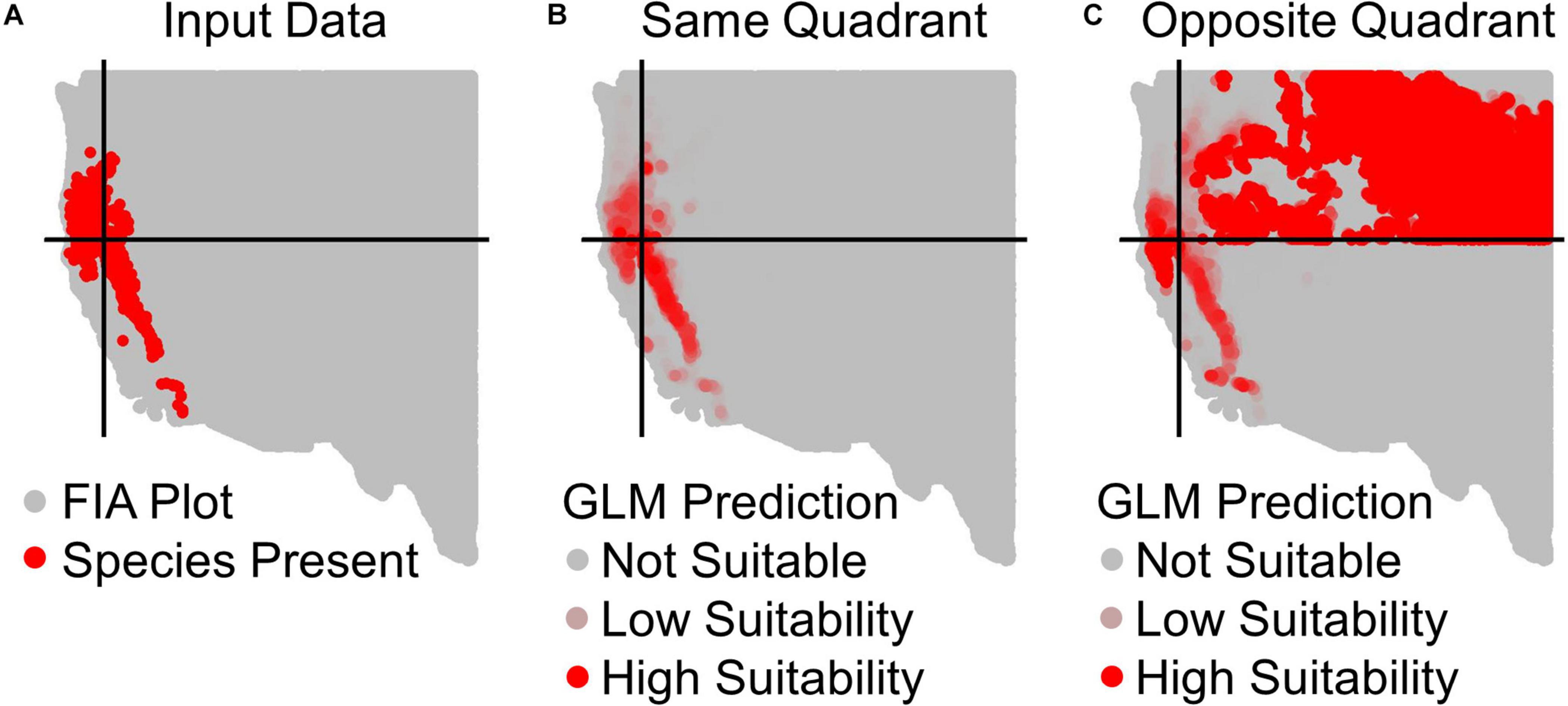
Figure 2. Example prediction maps for Calocedrus decurrens using GLM. (A) The input FIA plots, where red are presences and gray are absences. Black lines designate the median latitude and longitude of presence plots, dividing the geographic space into our four quadrants specific to this species. (B) GLM predictions within the same quadrant as training data, where the intensity of red denotes the continuous output of habitat suitability. (C) GLM prediction to the opposite quadrant from the training data. The extreme over-prediction seen here in the northeast quadrant of the novel region predictions was a recurrent pattern typical across all quadrants and algorithms, except for SRE.

Species Distribution Models

The term SDM covers a variety of types of models with different types of responses (e.g., presence-absence, presence-only, abundance) and predictor variables (e.g., climate, elevation, soil, location, other physiographic information). In this paper we consider SDMs that are often referred to as climate envelope or climatic niche models, wherein we only consider climatic predictor variables and a presence/absence response. We compared the predictive ability of 11 model algorithms contained within the Biomod2 version 3.1 package in R: Generalized Linear Model (GLM), Generalized Additive Model (GAM), Generalized Boosting Model (GBM), Classification Tree Analysis (CTA), Artificial Neural Network (ANN), Surface Range Envelop (SRE), Flexible Discriminant Analysis (FDA), Multiple Adaptive Regression Splines (MARS), Random Forest (RF), Maximum Entropy (Maxent), and an ensemble prediction based on these 11 algorithms (Thuiller et al., 2009, 2016). We considered this wide spectrum of algorithms to capture the range of feasible ways in which one might capture occurrence-environment relationships. A review of >200 published papers using biomod2 prior to 2016 showed that common practice by users of this software is to use the default tuning for algorithms (Hao et al., 2019). To maintain consistency with this general practice and given the computational infeasibility of tuning individual settings for the nearly 5000 individual SDMs that we fit in this study, we used biomod2 default tuning choices². Merow et al. (2014) have demonstrated that many of the 11 algorithms we considered can be made to produce very similar response curves to each other by choosing different combinations of settings. Our use of the default settings means that performance comparisons among algorithms in this study can best be interpreted as a comparison of response curves with differing complexity (cf. Merow et al., 2014) rather than an examination of which algorithm is best – since one algorithm may perform as well as another if different settings were chosen.

Evaluation of Model Transferability

Effect of SDM Algorithm Complexity on Geographic Transferability

To address Question 1, we tested each of the 11 model algorithm’s ability to predict species’ occurrence at points within the same geographic extent as points used for model training (holdout geographic transferability) and to points outside of the geographic extent used for model training (novel geographic transferability) by splitting our entire geographic region into four quadrants based on the median latitude and longitude of presence data for a given species (Figure 1A). For each of the four quadrants (northwest, northeast, southeast, southwest), we fit each algorithm using all FIA plots within that quadrant. We then used the algorithm to predict to the FIA plot locations in the opposite quadrant. This quadrant approach is a common method for partitioning data to test SDM transferability across space (Feng et al., 2019), especially to explore the possibility of encountering no-analog environmental conditions (Muscarella et al., 2014). For example, the fit to the northeast was used to predict to the southwest. To assess predictive performance, we measured the area under the receiver operating curve (AUC), sensitivity (1 – false negative rate), specificity (1 – false positive rate), and accuracy (ACC; the fraction of correct prediction i.e., the sum of true positives and true negatives divided by the total number of validation points; Fielding and Bell, 1997). To assess sensitivity and specificity, we first converted continuous model outputs to binary values using a threshold that optimized the sum of sensitivity and specificity (Liu et al., 2005; Lobo et al., 2008). We also used AUC to examine predictions to FIA plots in the same quadrant as the training data, once with the full set of FIA points used for both training and predicting, and once with 70% of the points used for training and 30% for testing.

We used ANOVA to test for significant differences in performance between the 11 algorithms we fitted that represented differing levels of SDM algorithm complexity (Question 1). Three separate ANOVAs with Type II sums of squares were fit to compare between SDM algorithm performance based on AUC, (1) across all plots used to train the models, (2) at testing plots not used to train the models, but within the same geographic extent as the training data, and (3) in a novel geographic extent. Three separate ANOVAs were also fit to assess SDM algorithm differences in ACC, true positive rates, and true negative rates in novel geographic extents. Fitting separate ANOVAs for these measures of predictive performance facilitated the interpretation of Tukey’s honestly significant differences (HSD) post hoc test. Because of occasional failures of algorithms to converge within biomod2, we ensured a balanced design by only including quadrant × species combinations in which the performance statistics yielded usable values for all models run. Failures to converge represented 1.6% of predictions to novel geographic regions and 9.0% of predictions to the training geographic region.

Limits to Extrapolation in Geographic and Environmental Space

To address Questions 2–4, we also examined the relationship between predictive performance and extrapolation distance outside the 19-dimensional climatic (i.e., environmental) space and outside the 2-dimensional geographic space of the training data. We measured the distance between every test FIA plot in the validation data and the centroid of the training data in the opposite quadrant (Figure 1). Distance was measured by first normalizing the distance along each variable axis, then calculating Euclidean distance, and finally dividing by the square root of the number of dimensions (i.e., two for geographic or number of climatic variables for environmental) to obtain a normalized distance in standard-deviation units. Within the testing quadrant, we binned the validation points, so that each bin would have enough points to confidently calculate goodness-of-fit metrics (e.g., AUC, ACC). To explore limits to extrapolation in geographic space, we binned points based on geographic proximity to the training region centroid, with 10,000 points per bin (Figure 1A). To explore limits to extrapolation in environmental space, we binned points based on proximity in environmental space to the fitting region centroid with 10,000 points per bin (Figure 1B).

We assessed goodness-of-fit of the models with two metrics: AUC and ACC. We note that AUC can be problematic as a predictive metric because it weights omission and commission errors equally (Lobo et al., 2008). AUC is more problematic when generating pseudoabsences with presence-only data, but less so when using presence/absence data as we use in this study. As such, we report both AUC and ACC (Lobo et al., 2008). To assess differences in limits to extrapolation of the SDMs in geographic space by algorithms, we fit two GLMs where the response was either AUC or ACC and algorithm (e.g., GLM, GAM, etc.) entered the GLMs as a fixed factor with geographic distance entered as a covariate. We also included an interaction between geographic distance and model algorithm to determine if algorithms varied at different rates in their ability to extrapolate in geographic distance. To assess limits to extrapolation of the SDMs in environmental space, we fit similar mixed effect models where the covariate was distance in environmental, rather than geographic, space. These GLMs were fit with Type III sums of squares given the inclusion of the interaction term. The data were analyzed with separate GLMs for AUC and ACC for geographic and climatic distance to facilitate the interpretation of Tukey’s HSD test. All R code and data used in the analyses along with the ODMAP (Overview, Data, Model, Assessment, and Prediction) protocol documenting the SDMs (Zurrell et al., 2020) are available on Figshare³.

Results

Question 1 – Overall Transferability Differences Among Algorithms

All results in figures presented in the main text are from the algorithm runs with the full suite of bioclimatic explanatory variables (see Supplementary Figures 2–8 for results from algorithms run with the subset of nine uncorrelated variables). Performance of all algorithms was qualitatively similar whether all bioclimatic predictors were used to fit the algorithms versus the subset of nine uncorrelated variables, except for GLM which had worse predictions when using only uncorrelated variables. Generally, all algorithms performed best when testing plots were located within the training region (Figure 2B) where average AUC values for all algorithms were >0.7 (Figure 3B). A substantial portion of predictions into novel regions for all algorithms performed worse than would be expected by random chance (Figures 2C, 3C and Table 1). When testing plots within the training region, the ranked AUC for random forest was much better than when predicting to a novel region, suggesting that the algorithms were overfit (Figure 3). When testing plots in novel geographic regions, the models with the highest mean AUC and the highest summed sensitivity and specificity were Maxent, GLM, and GAM (Figure 3). However, GLM had lower AUC, lower ACC, and higher true negative rates when run with uncorrelated variables (Supplementary Figures 2, 3). A common pattern across most algorithms was the tendency for extreme over-prediction in the novel regions, wherein species with narrow true ranges were predicted to occur at most plots (Figure 2C). The one exception to this pattern was SRE, which tended to make more conservative occurrence predictions for the novel region compared to the training region (Figure 4A). In both the training regions and the novel regions, all algorithms but SRE had false negative rates lower than expected by chance but false positive rates higher than expected (Figures 4B,C).

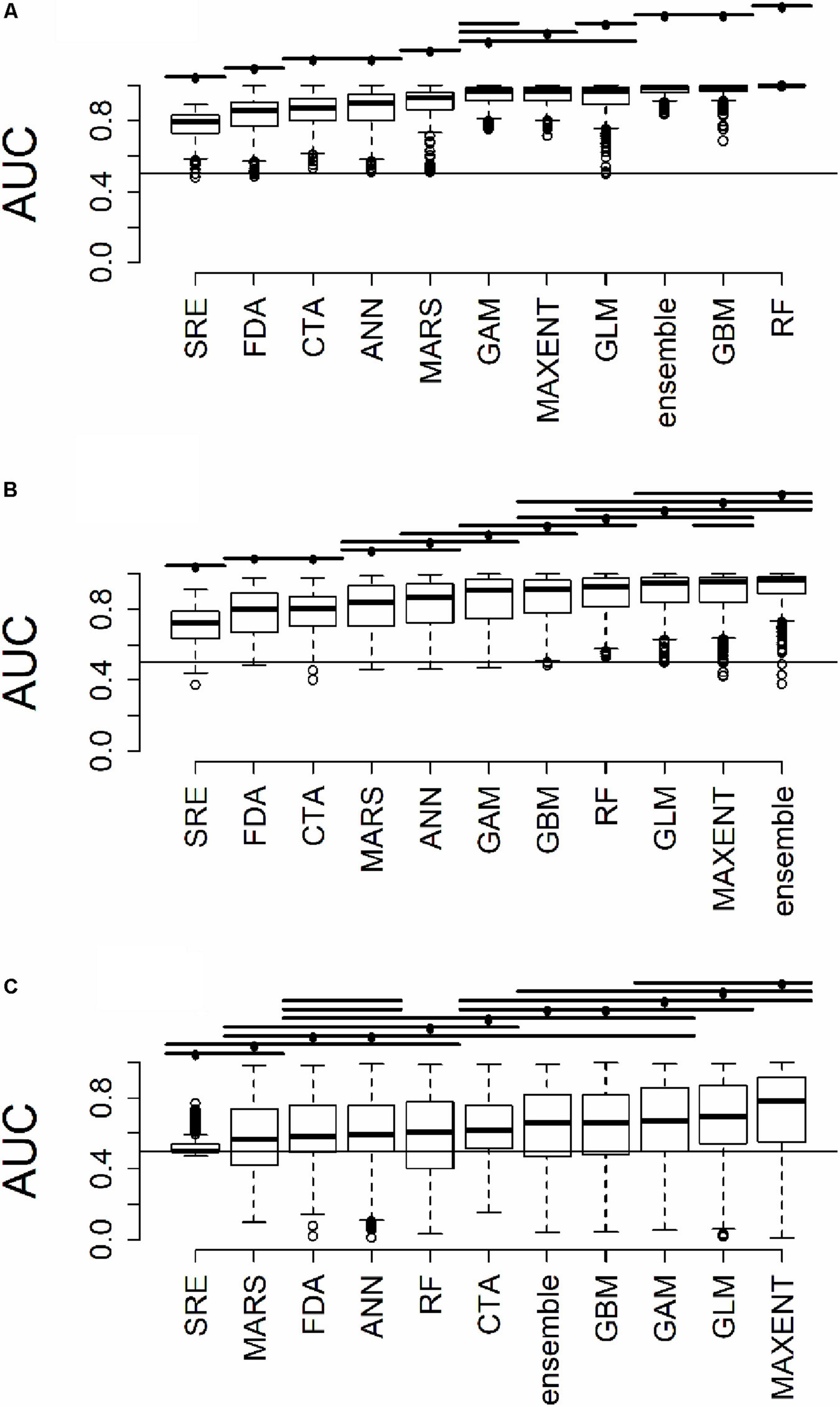
Figure 3. Distribution of AUC for model predictions (A) across all plots used to train the algorithms (B) at testing plots not used to train the algorithms, but within the same geographic extent as the training data, and (C) in a novel geographic extent. Horizontal bars above the boxplots represent significant Tukey post hoc groups. Black dots within the Tukey group bars represent the reference algorithm – all algorithms beneath a given bar are not significantly different from the reference algorithm for that bar. Multiple black dots on a given bar indicate that the Tukey groups are identical for multiple algorithms.

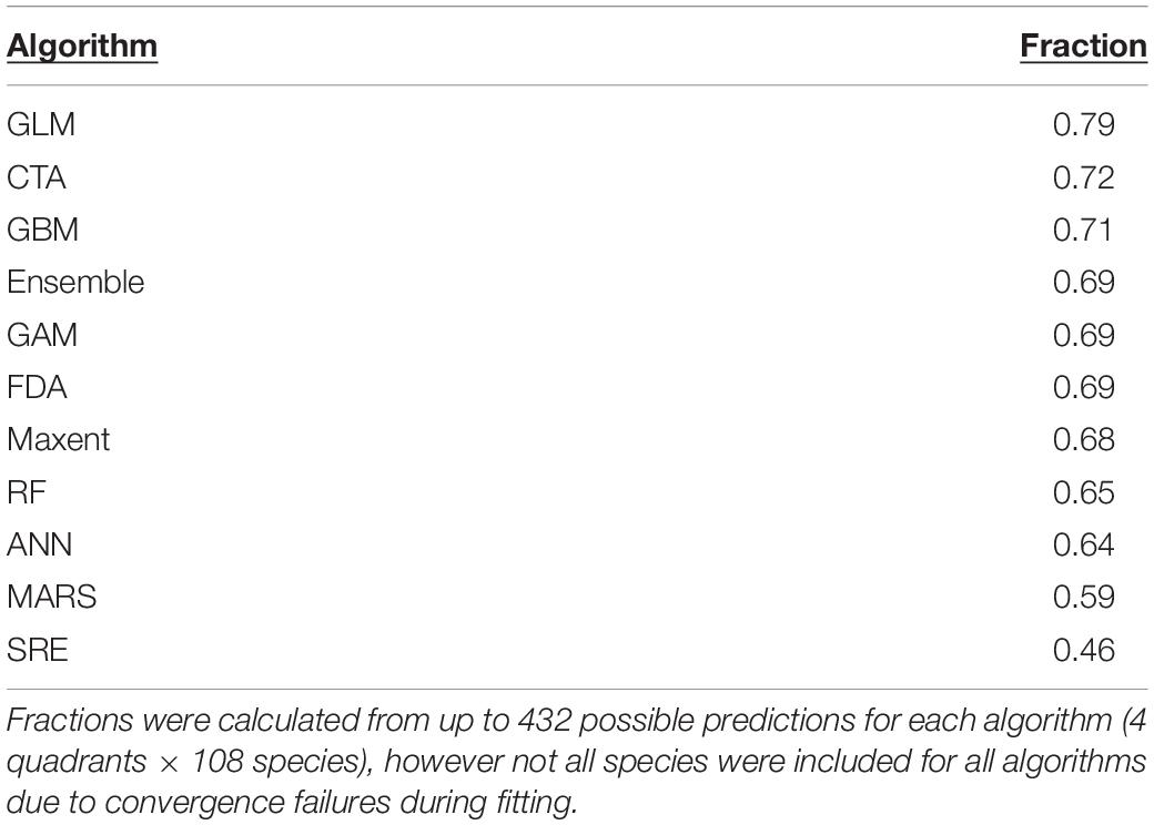
Table 1. Fraction of predictions to novel regions in which species distribution models performed better than random (AUC greater than 0.5).

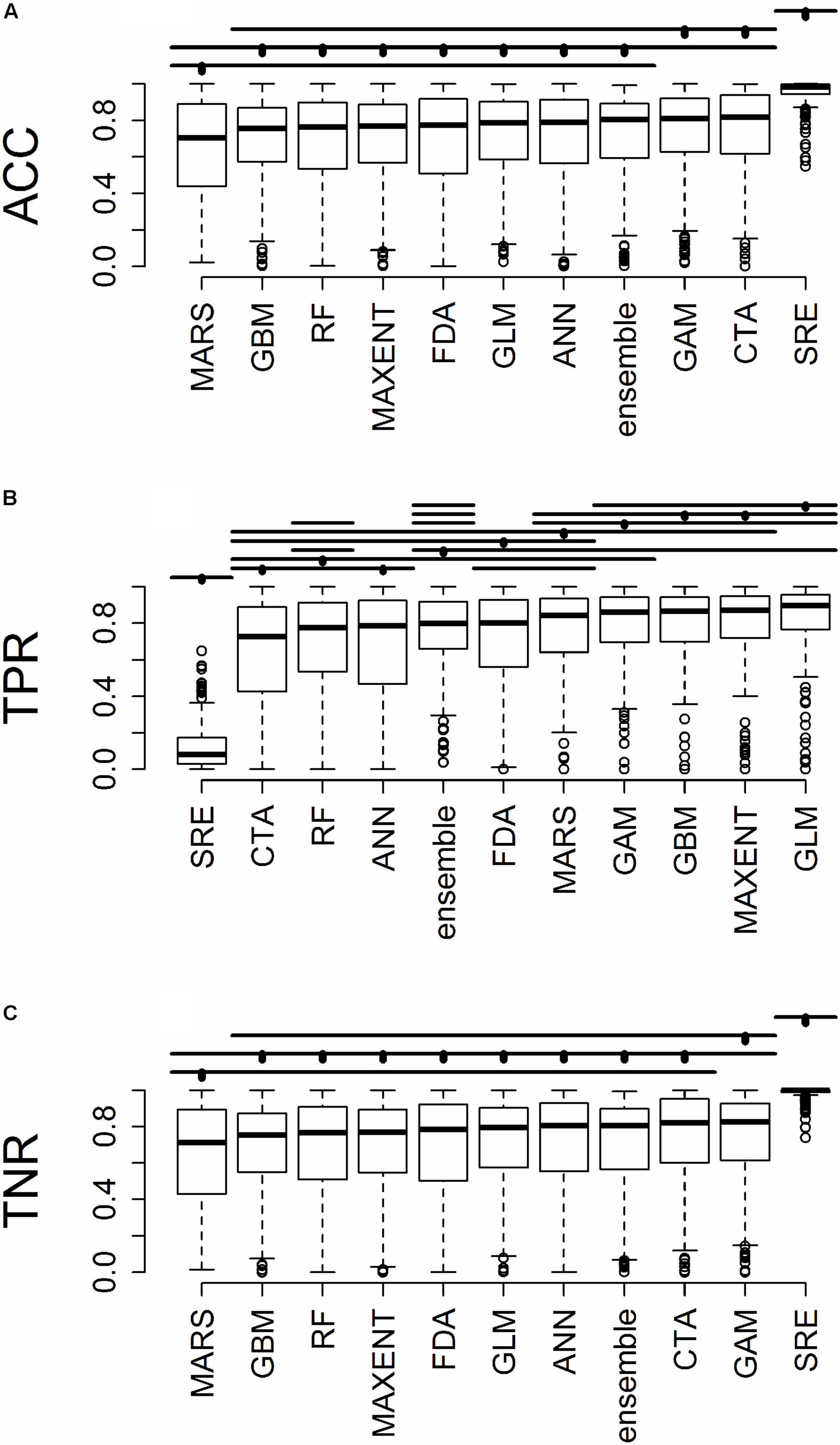
Figure 4. For predictions into novel geographic regions, the distribution of (A) accuracy (ACC), (B) true positive rate (TPR), and (C) true negative rate (TNR). Horizontal bars above the boxplots represent significant Tukey post hoc groups. Black dots within the Tukey group bars represent the reference algorithm – all algorithms beneath a given bar are not significantly different from the reference algorithm for that bar. Multiple black dots on a given bar indicate that the Tukey groups are identical for multiple algorithms.

Question 2 – Extrapolation Versus Distance in Geographic Space

Differences in the ability of SDMs to extrapolate in geographic space (i.e., where plots were binned based on geographic proximity to the training region centroid, with 10,000 plots per bin) depended on the metric of predictive performance used. The ability of SDMs to extrapolate in geographic space declined significantly with increasing distance from the fitting region when predictive performance was assessed with AUC (Figure 5A; F₁,₁₀₈₄₇ = 9.25, p < 0.005). However, the rate at which predictive performance declined with geographic distance was not significant when assessed with ACC (Figure 5C; F₁,₁₀₈₄₇ = 2.11, p > 0.1).

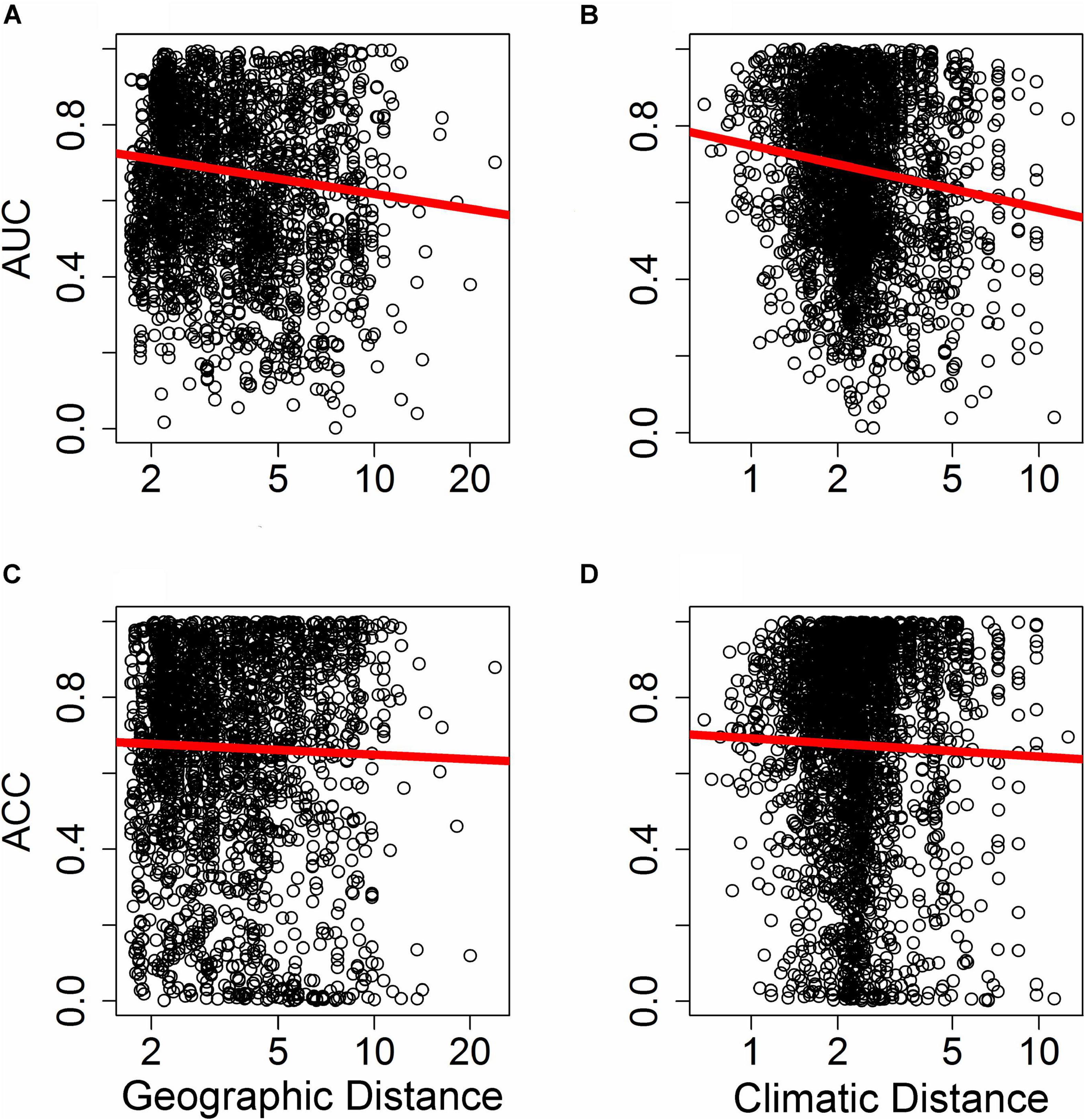
Figure 5. Effect of distance in environmental space on predictive ability of species distribution models (SDM), measured as AUC (A,B) or ACC (C,D). Each point represents AUC or ACC calculated within a single bin of up to 10,000 holdout points in a novel geographic region binned by distance through either geographic space (A,C) or environmental space (B,D) from the fitting region for one quadrant of a given species and a given SDM algorithm. Distance was measured by first normalizing the distance along each variable axis, then calculating Euclidean distance, and finally dividing by the square root of the number of dimensions (i.e., two for geographic space and 19 for climatic space) to obtain a normalized distance in standard-deviation units. The regression line represents a GAM fit to the data.

Question 3 – Extrapolation Versus Distance in Environmental Space

Differences in the ability of SDMs to extrapolate in environmental space were more consistent and significant across metrics of predictive performance used. The ability of SDMs to extrapolate in environmental space declined significantly with increasing distance from the fitting region when model performance was assessed with both AUC (Figure 5B; F₁,₁₅₅₆₃ = 18.84, P < 1.4 × 10^–5) and ACC (Figure 5D; F₁,₁₅₅₆₃ = 6.70, P < 0.01).

Question 4 – Differences Among Algorithms in Extrapolation Versus Distance

When SDMs were extrapolated in geographic space, there were no significant differences in predictive performance as measured by AUC between algorithms (F₁₀,₁₀₈₄₇ = 10.6, p = 0.4) nor was there an interaction between algorithms and distance of extrapolation in geographic space (F₁₀,₁₀₈₄₇ = 2.63, p = 0.99; Figure 6). Similarly, there were no significant differences in predictive performance as measured by ACC between algorithms (F₁₀,₁₀₈₄₇ = 16.8, p = 0.08) nor was there an interaction between algorithms and distance of extrapolation in geographic space (F₁₀,₁₀₈₄₇ = 5.45, p = 0.86; Supplementary Figure 9).

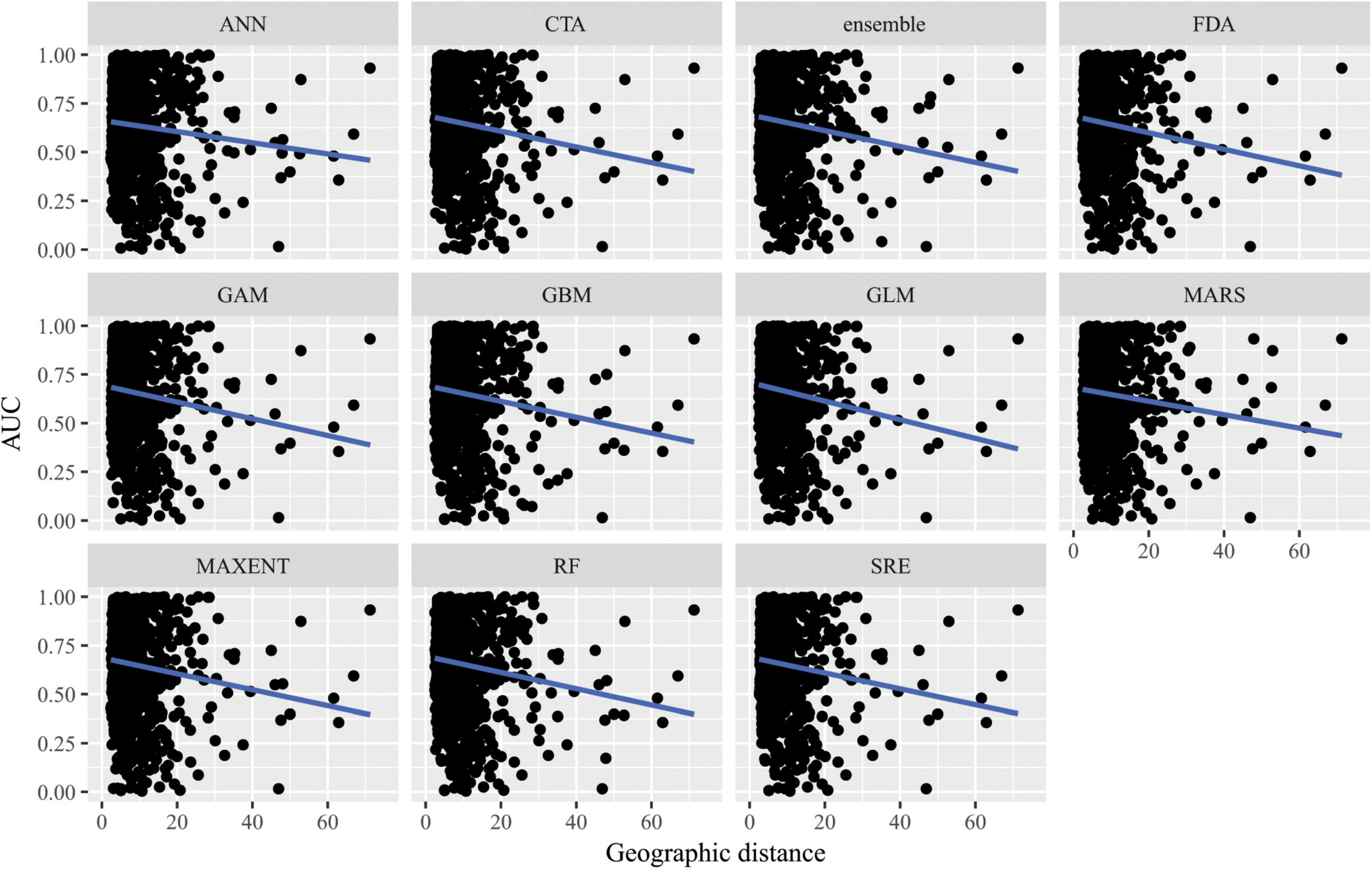
Figure 6. Predictive performance of species distribution models with different algorithms as measured with AUC versus distance of extrapolation in geographic space in a novel geographic region. Distance was measured by first normalizing the distance along each variable axis, then calculating Euclidean distance, and finally dividing by the square root of the number of dimensions (i.e., 2) to obtain a normalized distance in standard-deviation units.

When SDMs were extrapolated in environmental space, there were significant differences in predictive performance as measured by AUC between algorithms (F₁₀,₁₅₅₆₃ = 21.2, p = 0.02), but post hoc comparisons revealed that these were mainly driven by differences in predictive ability between Maxent and artificial neural network algorithms. There was a significant interaction between algorithms and distance of extrapolation in environmental space (F₁₀,₁₅₅₆₃ = 27.1, p = 2.5 × 10^–3; Figure 7). In particular, the following algorithms’ predictive capacities declined steeply with increasing extrapolation in environmental space relative to other algorithms: FDA, GAM, Maxent, and SRE. When ACC was used as the measure of predictive performance for extrapolation in environmental space, there was a significant interaction between algorithm and distance of extrapolation in environmental space (F₁₀,₁₅₅₆₃ = 22.1, p = 0.01; Supplementary Figure 10), but differences between algorithms alone were not significant (F₁₀,₁₅₅₆₃ = 17.8, p = 0.06). Averaged across all measures of predictive performance (i.e., AUC, ACC, true positive rates, and true negative rates) and across all species for transfers in environmental space, GAM had the best performance whether or not the full set of predictor variables or a reduced set of non-collinear predictor variables were used to fit the models.

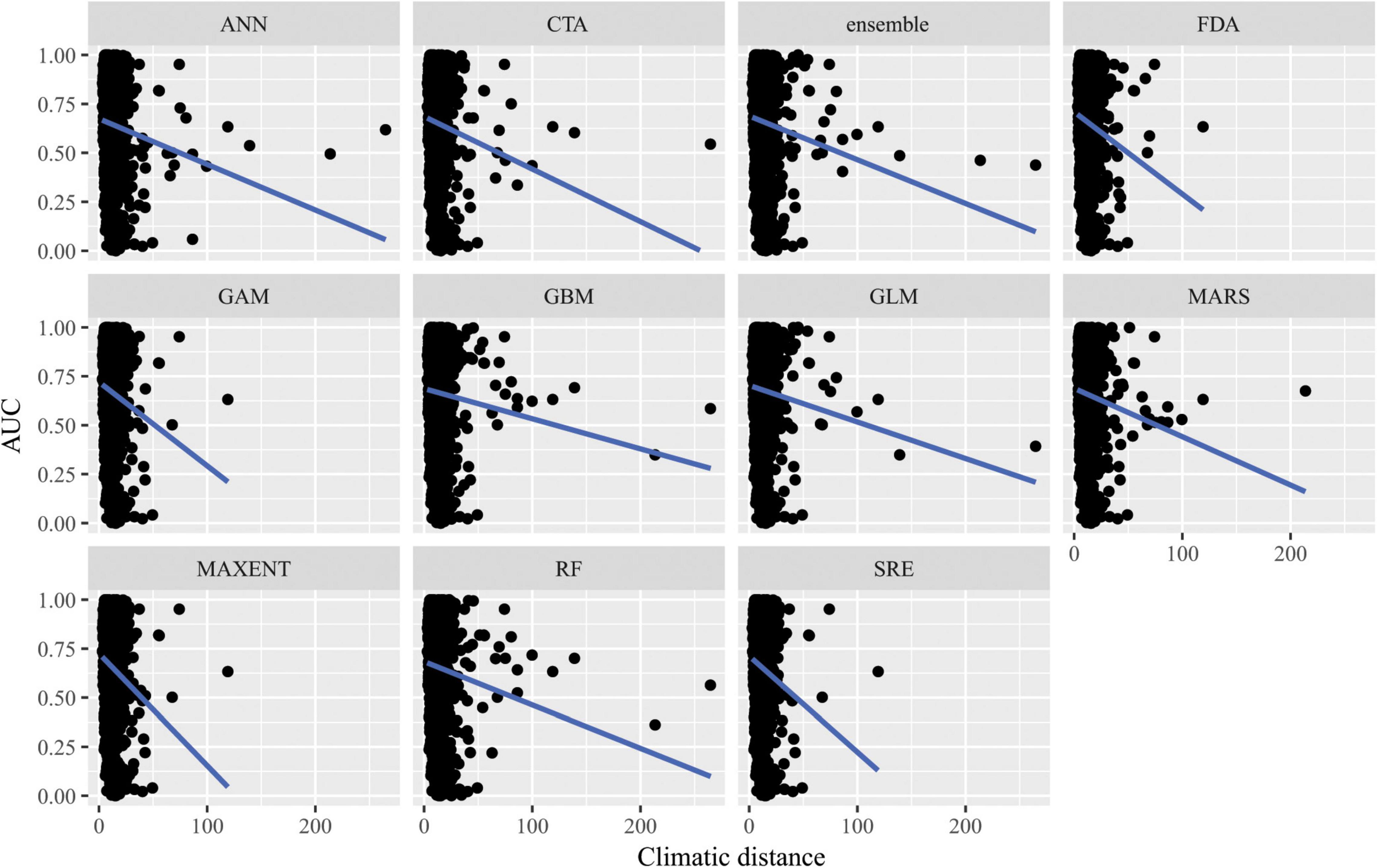
Figure 7. Predictive performance of species distribution models with different algorithms as measured with AUC versus distance of extrapolation in environmental space in a novel geographic region. Distance was measured by first normalizing the distance along each variable axis, then calculating Euclidean distance, and finally dividing by the square root of the number of dimensions (i.e., 19) to obtain a normalized distance in standard-deviation units.

Discussion

Species distribution models can be an important tool for conservation by predicting range shifts as a consequence of global change (Elith and Leathwick, 2009; Franklin, 2010). Maps of potential range shifts can be essential for prioritizing reserves across landscapes, however, in some cases, the pressing need for conservation action can outweigh the caution necessary to properly interpret these predictions (Fitzpatrick and Hargrove, 2009; Jimenez-Valverde et al., 2011; Sequeira et al., 2018). As the appearance of no-analog climates is predicted to rise over the next century (Williams and Jackson, 2007), more research is necessary to understand the limitations of SDM transferability in geographic and environmental space. Thus far, transferability of SDMs to new time periods, geographic regions, and determining cross-taxa caveats, have shown inconsistent patterns that could be due to myriad factors (e.g., model algorithms, input data, parameterization). This lack of progress has prompted the call for more rigorous testing to learn about the limitations of extrapolation in geographic and environmental space, and to help establish general guidelines for model transfer (Yates et al., 2018). In this study, we explicitly tested the ability of SDMs of varying complexity to transfer in both geographic and environmental space for data rich tree species in the western United States. Our approach of fitting models in one quadrant of geographic space and predicting them in another quadrant of geographic space is a stringent test that may be akin to projecting occupancy under no-analog conditions that may arise in the western United States with climatic change (Williams and Jackson, 2007). We found that SDMs for this system and geographic region tend not to be transferable in geographic or environmental space. Furthermore, distance in environmental space determined predictive performance of the SDMs more than distance in geographic space or the type of algorithm used.

When interpreting the results of this study, it is important to note that the predictive performance metrics we used are not perfect. We note that, although commonly used for model performance evaluations, AUC, sensitivity, specificity, and ACC can be misleading (Lobo et al., 2008; Pontius and Parmentier, 2014). For instance, AUC is impacted by the “extent to which models are carried out,” describes predictive performance across portions of the Receiver Operating Curve (ROC) space which may be biologically infeasible, weights commission and omission errors the same, fails to consider predicted probability outputs and model goodness-of-fit, and ignores the spatial distribution of model errors (Lobo et al., 2008). Future studies might consider other model predictive performance measures, such as graphical assessment of curves representing the Total Operating Characteristic (Pontius and Si, 2014), which provide a richer assessment of the information contained in the ROC. This approach was not taken in this study because it would have necessitated a visual interpretation of thousands of curves (1 model algorithms × 108 species × 2 tests × 4 quadrants = 9504 curves). Future work that automates graphical interpretation or provides summary metrics describing the shape of the TOC curve, without loss of information, would make the use of these more sophisticated metrics possible for studies assessing many species across various model algorithms and tests of transferability.

Furthermore, the interpretation of the results of this study may be strongly dependent upon the field of study and understood purpose of SDMs. Averaged across many species, most algorithms with default tuning settings had median AUC values near 0.7 when applied to novel geographic regions in our study (Figure 3C). From a statistical perspective, this indicates that, on average, SDMs are informative. As a tool for developing and testing fundamental theories in ecology and evolution, this may be sufficient. Users at that level are often tuning algorithms beyond the default settings and/or including additional predictor variables (e.g., remotely sensed elevation, soils, other physiographic variables) and may thus achieve much better predictive performance (Guisan et al., 2007; Austin and Van Niel, 2011). However, the ultimate purpose for many SDMs is applied conservation – where many end-users of SDMs may not be aware of available non-climatic spatial data layers (Zarnetske et al., 2019) nor have the training or capacity to tune algorithms beyond the available default settings or to fully appreciate their statistical limitations. When predicting beyond the geographic area used for training, the algorithms in our study performed worse than random about 30% of the time for many of the commonly employed algorithms (Table 1). This may be an unacceptably high rate of failure for SDMs to serve as a useful tool for guiding individual species conservation. Determining policy and management decisions based on such unreliable predictions could be dangerously counterproductive. Imagine, for instance, designing reserve boundaries for high-profile endangered species using such models in unsampled regions. For one out of three species, the SDMs are likely to suggest reserve boundaries that capture fewer presences than if we were to blindly select arbitrary polygons from across the entire available map. With such odds, a manager may be better served by circling areas on a paper topographic map based on their own natural history understanding of the system.

Question 1 – Overall Transferability Differences Among Algorithms

When predicting species occurrence in novel regions, some algorithms performed better in terms of mean AUC and the highest summed sensitivity (e.g., Maxent, GLM, GAM; Figure 3; see also Heikkinen et al., 2012; Wenger and Olden, 2012). Maxent may have performed well in most cases because the default settings of biomod2 use threshold and hinge settings. These settings make a continuous environmental predictor binary by forcing responses to zero below a certain value and to one above that value (Merow et al., 2014). GLM had lower AUC, lower ACC, and higher true negative rates when run with uncorrelated variables (Supplementary Figures 2, 3) compared to the full suite of 19 correlated bioclimatic variables (Figures 3, 4). The default settings for biomod2 allow for Akaike Information Criterion (AIC) variable selection within GLM. It is possible that the reduced set of nine bioclimatic variables contained explanatory variables with relatively weak relationships to species occurrence compared to some of the explanatory variables maintained in the full set of 19 bioclimatic variables. Thus, when AIC model selection occurred for the uncorrelated set of variables, there was selection bias where the parameters were poorly estimated for those explanatory variables with weak relationships to the occurrence response, resulting in poor predictive ability (Lukacs et al., 2010).

Questions 2 and 3 – Extrapolation Versus Distance in Geographic and Environmental Space

Decay in model performance with increasing geographic distance from training data depended on predictive performance metric (AUC and ACC in Figure 5). In contrast, as climatic distances became more dissimilar to training data, model performance declined significantly regardless of predictive performance metrics (AUC and ACC values in Figure 5). These results indicate a decay in predictive ability of algorithms in increasingly environmentally dissimilar regions. Further, the number of false negatives were consistently lower than the number of false positives expected by chance (i.e., higher true negative rate and lower true positive rate; Figure 4), showing a trend toward strong overprediction in novel regions, even for narrow ranged species (Figure 2C). These findings suggest that algorithms for this system and geographic region tend not to be transferable, particularly in environmental space. However, we also note that the opposite quadrant data partitioning approach used here to test SDM transferability is stringent. Different partitions of the training and testing data (e.g., if the training and testing quadrants had similar longitudinal bounds or using three of the four quadrants for training and one for testing) may have had better predictive performance in tests of transferability, and would be very informative as follow up-studies.

Question 4 – Differences Among Algorithms in Extrapolation Versus Distance

Our results suggest that for transfers in geographic space, no specific algorithm was better than another as there were no significant differences in predictive performance as measured by AUC or ACC across algorithms. However, there were significant differences in predictive performance for algorithms transferred in environmental space. Of the algorithms assessed, GAM performed best in transferring in environmental space, but it is important to note that GAMs’ performance declined steeply with increasing extrapolation in environmental space relative to other algorithms.

Beyond model complexity, other potential reasons may explain the poor transferability of the models. For example, species-specific tuning can improve transferability in novel regions and climates (Guevara et al., 2018). Tuning has been shown to generate more realistic SDMs as opposed to using default settings (as used here). However, species-specific tuning of SDMs in training does not necessarily equate to better transferability to novel environments because the observed correlative species occurrence and environment relationship provides no insight into how the species will respond to no-analog conditions (Fitzpatrick and Hargrove, 2009; Heikkinen et al., 2012; Sequeira et al., 2018). In the future, the western United States is likely to experience no-analog climates, especially in regions of California (Williams and Jackson, 2007). Thus, tuning to specific species’ current climate envelopes and predicting to future climates would not necessarily help in our study region, as any prediction would lead to strong extrapolation beyond current and paleo climatic conditions and therefore increase uncertainty in model predictions. Another potential explanation for poor transferability is the geographic partitioning of species occurrence records by the median latitude and longitude of points to determine the four testing quadrants. A common method of cross validation, dividing species occurrence records and training algorithms in quadrants results in likely truncation of the species full climate envelope (Muscarella et al., 2014). This can result in incomplete response curves in model training, leading to poor transferability (Thuiller et al., 2004; Owens et al., 2013; Guevara et al., 2018). Different partitions of the training and testing data (e.g., if the training and testing quadrants had similar longitudinal bounds or using three of the four quadrants for training and one for testing) may have led to better predictive performance in tests of transferability. Comparison of paleoclimatic and current climatic records compared to predicted future climatic conditions in our study extent suggest that no-analog climatic conditions are highly probable for this region of North America (Williams and Jackson, 2007), thus, our approach to testing transferability simulates the real-world challenge of predicting to a future using data that may not encompass the full breadth of species’ niches.

Conclusion and Future Directions

Understanding the limits to extrapolation for SDMs is important for biodiversity assessments (e.g., International Union for Conservation of Nature criteria) since future predictions of species distributions are often considered. The ability of decision makers to spatially plan conservation actions based on SDM predictions across time and space (environmental or geographic) relies on the transparency and documentation of the modeling approaches, including the degree of extrapolation and uncertainty (Sequeira et al., 2018). Assessing and communicating the uncertainty of these predictions to potential stakeholders avoids the misallocation of resources for conservation in regions where predictions are questionable (e.g., areas of strong overprediction; Figure 2C). For instance, Houlahan et al. (2017) suggested that when transferring models, there must be a minimum degree of similarity between the environmental conditions of the training and testing region for that prediction to be interpreted with a modicum of confidence. A possible solution to the lack of certainty of these predictions transferred to different times or regions is for modelers to delineate a “forecast horizon,” or a threshold which demarcates a point at which predictions are too uncertain and likely no longer useful (Petchey et al., 2015). Though we did not explicitly do this here, this can easily be achieved in future studies by using a measure of performance and defining what is an acceptable level of algorithm performance quality (e.g., AUC, degree of environmental overlap between training and testing regions).

Given the results of this study, there is a strong need for more tests of algorithm transferability across taxa in different regions of the world. By increasing our understanding of limits to transferability within different regions and study systems, guidelines can be established on the appropriate use and interpretation of algorithm transfer. There would also be value to comparing the transferability of SDMs where the response variable is presence/absence or presence only to models where the response variable is non-binary (e.g., abundance, basal area for trees). Simplifying habitat suitability to a binary response may not be biologically realistic when there may be various reasons why a location is predicted to be suitable but the species is absent or why a species is detected but at that location it generally has trouble regenerating.

Though here we mainly discuss correlative SDMs in terms of transferability, mechanistic models, or models that incorporate biological processes that limit and shape species distributions (e.g., dispersal, biotic interactions, population dynamics; Belmaker et al., 2015; Buckley and Catford, 2016; Record and Charney, 2016) hold much promise and can potentially achieve higher transferability (Evans et al., 2016). However, these process-based models require abundant experimental data, are computationally intensive, and the influence of mechanisms added into such models may only operate at particular spatial scales, which has caused progress in this field to be slow thus far (Record et al., 2018; Sequeira et al., 2018) and therefore they too require further study within the context of transferability. There also may be great value to combining occurrence based correlative SDMs with process-based SDMs.

We also note that it is relevant to consider model transferability, even if the goal of conservation is not focused on an individual, often rare, species. In the last decade, some conservation efforts have begun to focus less on where individual species may shift their geographic ranges and more on specific attributes of Earth’s surface that promote diversity of a large number of species (Lawler et al., 2015). This latter approach is often referred to as ‘conserving nature’s stage’ wherein the organisms are the actors, and the stage is Earth’s environment. The goal is to identify areas with higher habitat diversity that may harbor higher levels of biodiversity. This habitat diversity is termed geodiversity—variation in Earth’s abiotic processes and features; (Zarnetske et al., 2019; Record et al., 2020). Schrodt et al. (2019) recently called for the international groups (e.g., the Group on Earth Observations Biodiversity Observation Network [GEOBON]) to consider a framework for identifying essential geodiversity variables (EGV) to complement the essential biodiversity variables (EBV) framework that places a strong emphasis on understanding potential changes in species distributions (Pereira et al., 2013). Ultimately, a focus on geodiversity still requires an understanding of the relationships between biodiversity and geodiversity across space and time (Read et al., 2020), which will also need to consider transferability of models linking geodiversity to biodiversity.

Moving forward, the decision to focus more on process based SDMs or geodiversity of parcels will depend on the regulatory bounds of any conservation organization. For instance, an emphasis on species distributions makes sense for legislation protecting species (e.g., the United States Endangered Species Act), whereas individual organizations purchasing land holdings may want to take the geodiversity and ‘conserving nature’s stage’ approach. Regardless, process-based SDMs and models of geodiversity-biodiversity relationships necessitate the same understanding of how the models will transfer in space and time to conserve nature now and into the future.

Data Availability Statement

Publicly available datasets were analyzed in this study (Record et al., 2021). The following .csv and .Rdata files contain Forest Inventory and Analysis and climate data required to reproduce the analysis: REF_SPECIES.csv, all_FIA_locations.csv, all_FIA_presences.csv, and all_locations_data_2.R. The following .R files are R scripts, tested under R/3.1, that contain code to reproduce the analyses in the manuscript: climate_data_code.R, SDM_analyses.R. The Biomod default settings.Rmd file contains information on the default settings of biomod2 used in the analyses.

Author Contributions

NDC, SR, and CM conceived the study. NDC and SR performed analyses. SR and BG led the writing. All authors interpreted results and edited drafts.

Funding

The Bryn Mawr K.G. Fund provided support for SR. Michigan State University and NASA #80NSSC19K1332 supported BG and PZ. CM acknowledges funding from NSF Grants DBI-1913673 and DBI1661510 and NASA Grant and NASA ROSES award 80NSSCK0406. NDC and BJE were supported in part by a fellowship from the Aspen Center for Environmental Studies to BJE. BJE was supported by National Science Foundation award DEB 1457812 and a Conservation International SPARC award.

Conflict of Interest

The authors declare that the research was conducted in the absence of any commercial or financial relationships that could be construed as a potential conflict of interest.

Acknowledgments

This project was supported by the USDA National Institute of Food and Agriculture, Hatch (or McIntire-Stennis, Animal Health, etc.) Project number ME0-42212 through the Maine Agricultural & Forest Experiment Station. Maine Agricultural and Forest Experiment Publication Number 3822. We thank the United States Forest Service for maintaining the Forest Inventory and Analysis data collection effort.

Supplementary Material

The Supplementary Material for this article can be found online at: https://www.frontiersin.org/articles/10.3389/fevo.2021.689295/full#supplementary-material

Supplementary Figure 1 | Correlations between bioclimatic variables.

Supplementary Figures 2–8 | Results of analyses run with reduced set of nine uncorrelated bioclimatic explanatory variables.

Supplementary Figures 9–10 | ACC versus geographic or climatic distance for analyses run with unreduced set of correlated bioclimatic explanatory variables.

Supplementary Data Sheet 1 | List of 108 tree species fitted with species distribution models. Abbreviations are as follows: count (number of presences within study extent), species symbol (species code comprises the first two letters of generic and specific epithets), genus, species, variety, and subspecies.

Supplementary Data Sheet 2 | Performance of species distribution models in predicting presence or absence of tree species at Forest Inventory and Analysis (FIA) plots. Ten different algorithms (“Algorithm” column) including the ensemble forecast were applied to 108 species (“Species” column). For each species, the landscape was divided into four regions based on the cardinal quadrants (NE, SE, SW, NW in “Quadrant” column) for fitting each algorithm. Model performance was evaluated in either the fitting quadrant (“self” in “TestQuadrant” column) or on the diagonally opposite quadrant (“opp”). Performance metric evaluated here is the area under the receiver operating curve (“AUC” column).

Supplementary Data Sheet 3 | Supplementary Figures.

Footnotes

1. ^ https://cds.nccs.nasa.gov/nex/
2. ^ https://doi.org/10.6084/m9.figshare.c.5360402
3. ^ https://doi.org/10.6084/m9.figshare.c.5360402

References

Anderson, R. P. (2013). A framework for using niche models to estimate impacts of climate change on species distributions: niche models and climate change. Ann. N. Y. Acad. Sci. 1297, 8–28. doi: 10.1111/nyas.12264
Austin, M. P., and Van Niel, K. P. (2011). Improving species distribution models for climate change studies: variable selection and scale. J. Biogeogr. 38, 1–8. doi: 10.1111/j.1365-2699.2010.02416.x
Bahn, V., and McGill, B. J. (2013). Testing the predictive performance of distribution models. Oikos 122, 321–331. doi: 10.1111/j.1600-0706.2012.00299.x
Bechtold, W. A., and Peterson, P. L. (2005). The Enhanced Forest Inventory and Analysis Program – National Sampling Design and Estimation Procedure. General Technical Report SRS-80. Asheville, N.C: US Department of Agriculture, Forest Service.
Belmaker, J., Zarnetske, P., Tuanmu, M.-N., Zonneveld, S., Record, S., Strecker, A., et al. (2015). Empirical evidence for the scale dependence of biotic interactions: scaling of biotic interactions. Glob. Ecol. Biogeogr. 24, 750–761. doi: 10.1111/geb.12311
Botkin, D. B., Saxe, H., Araújo, M. B., Betts, R., Bradshaw, R. H. W., Cedhagen, T., et al. (2007). Forecasting the effects of global warming on biodiversity. BioScience 57, 227–236. doi: 10.1641/B570306
Brown, J. L. (2014). SDMtoolbox: a python-based GIS toolkit for landscape genetic, biogeographic and species distribution model analyses. Methods Ecol. Evol. 5, 694–700. doi: 10.1111/2041-210X.12200
Brun, P., Thuiller, W., Chauvier, Y., Pellissier, L., Wüest, R. O., Wang, Z., et al. (2020). Model complexity affects species distribution predictions under climate change. J. Biogeogr. 47, 130–142. doi: 10.1111/jbi.13734
Buckley, Y. M., and Catford, J. (2016). Does the biogeographic origin of species matter? Ecological effects of native and non-native species and the use of origin to guide management. J. Ecol. 104, 4–17. doi: 10.1111/1365-2745.12501
Chapin, F. S. III, Zavaleta, E. S., Eviner, V. T., Naylor, R. L., Vitousek, P. M., Reynolds, H. L., et al. (2000). Consequences of changing biodiversity. Nature 405, 234–242. doi: 10.1038/35012241
Daly, C., Neilson, R. P., and Phillips, D. L. (1994). A statistical-topographic model for mapping climatological precipitation over mountainous terrain. J. Appl. Meteorol 33, 140–158.
Dirnböck, T., Dullinger, S., and Grabherr, G. (2003). A regional impact assessment of climate and land-use change on alpine vegetation: alpine vegetation change. J. Biogeogr. 30, 401–417. doi: 10.1046/j.1365-2699.2003.00839.x
Dormann, C. F., Elith, J., Bacher, S., Buchmann, C., Carl, G., Carré, G., et al. (2013). Collinearity: a review of methods to deal with it and a simulation study evaluating their performance. Ecography 36, 27–46. doi: 10.1111/j.1600-0587.2012.07348.x
Duncan, R. P., Cassey, P., and Blackburn, T. M. (2009). Do climate envelope models transfer? a manipulative test using dung beetle introductions. P. R. Soc. B Biol. Sci. 276, 1449–1457. doi: 10.1098/rspb.2008.1801
Elith, J., Graham, C. H., Anderson, R. P., Dudík, M., Ferrier, S., Guisan, A., et al. (2006). Novel methods improve prediction of species’ distributions from occurrence data. Ecography 29, 129–151. doi: 10.1111/j.2006.0906-7590.04596.x
Elith, J., and Leathwick, J. R. (2009). Species distribution models: ecological explanation and prediction across space and time. Ann. Rev. Ecol. Evol. Syst. 40, 677–697. doi: 10.1146/annurev.ecolsys.110308.120159
Evans, M. E. K., Merow, C., Record, S., McMahon, S. M., and Enquist, B. J. (2016). Towards process-based range modeling of many species. Trends Ecol. Evol. 31, 860–871. doi: 10.1016/j.tree.2016.08.005
Feng, X., Park, D. S., Liang, Y., Pandey, R., and Papes, M. (2019). Collinearity in ecological niche modeling: Confusions and challenges. Ecol. Evol. 9, 10365–10376. doi: 10.1002/ece3.5555
Fielding, A. H., and Bell, J. F. (1997). A review of methods for the assessment of prediction errors in conservation presence/absence models. Environ. Conserv. Null 24, 38–49.
Fitzpatrick, M. C., and Hargrove, W. W. (2009). The prediction of species distribution models and the problem of non-analog climate. Biodiv. Cons. 18, 2255–2261.
Franklin, J. F. (2010). Mapping Species Distributions, 1st Edn. New York, NY: Cambridge University Press.
Gillespie, A. J. R. (1999). Overview of the annual inventory system established by FIA. J. For. 97, 16–20.
Guevara, L., Gerstner, B. E., Kass, J. M., and Anderson, R. P. (2018). Toward ecologically realistic predictions of species distributions: a cross-time example from tropical montane cloud forests. Glob. Change Biol. 24, 1511–1522. doi: 10.1111/gcb.13992
Guisan, A., Zimmerman, N. E., Elith, J., Graham, C. H., Phillips, S., and Peterson, A. T. (2007). What matters for predicting the occurrence of trees: techniques, data, or species’ characteristics? Ecol. Monogr. 77, 615–630. doi: 10.1890/06-1060.1
Hannemann, H., Willis, K. J., and Macias-Fauria, M. (2016). The devil is in the detail: unstable response functions in species distribution models challenge bulk ensemble modelling: unstable response functions in SDMs. Glob. Ecol. Biogeogr. 25, 26–35. doi: 10.1111/geb.12381
Hao, T., Elith, J., Guillera-Arroita, G., and Lahoz-Monfort, J. J. (2019). A review of evidence about use and performance of species distribution modelling ensembles like BIOMOD. Divers. Distrib. 25, 839–852. doi: 10.1111/ddi.12892
Heikkinen, R. K., Marmion, M., and Luoto, M. (2012). Does the interpolation accuracy of species distribution models come at the expense of transferability? Ecography 35, 276–288. doi: 10.1111/j.1600-0587.2011.06999.x
Hijmans, R. J., Phillips, S., Leathwick, J., and Elith, J. (2020). Dismo: Species Distribution Modeling (version 1.3-3). Vienna: R Statistical Software.
Houlahan, J. E., McKinney, S. T., Anderson, T. M., and McGill, B. J. (2017). The priority of prediction in ecological understanding. Oikos 126, 1–7. doi: 10.1111/oik.03726
Ibáñez, I., Silander, J. A., Wilson, A. M., LaFleur, N., Tanaka, N., and Tsuyama, I. (2009). Multivariate forecasts of potential distributions of invasive plant species. Ecol. Appl. 19, 359–375. doi: 10.1890/07-2095.1
Jimenez-Valverde, A., Peterson, A. T., Soberon, J., Overton, J. M., Aragon, P., and Lobo, J. M. (2011). Use of niche models in invasive species risk assessments. Biol. Inv. 13, 2785–2797. doi: 10.1007/s10530-011-9963-4
Kass, J. M., Vilela, B., Aiello-Lammens, M. E., Muscarella, R., Merow, C., and Anderson, R. P. (2018). WALLACE?: a flexible platform for reproducible modeling of species niches and distributions built for community expansion. Methods Ecol. Evol. 9, 1151–1156. doi: 10.1111/2041-210X.12945
Kindsvater, H. K., Dulvy, N. K., Horswill, C., Juan-Jordá, M.-J., Mangel, M., and Matthiopoulos, J. (2018). Overcoming the data crisis in biodiversity conservation. Trends Ecol. Evol. 33, 676–688. doi: 10.1016/j.tree.2018.06.004
Lawler, J. J., Ackerly, D. D., Albano, C. M., Anderson, M. G., Dobrowski, S. Z., Gill, J. L., et al. (2015). The theory behind, and the challenges of, conserving nature’s stage in a time of rapid change: conserving nature’s stage in a time of rapid change. Conserv. Biol. 29, 618–629. doi: 10.1111/cobi.12505
Lembrechts, J. J., Lenoir, J., Roth, N., Hattab, T., Milbau, A., Haider, S., et al. (2019). Comparing temperature data sources for use in species distribution models: from in-situ logging to remote sensing. Glob. Ecol. Biogeogr. 28, 1578–1596. doi: 10.1111/geb.12974
Liu, C., Berry, P. M., Dawson, T. P., and Pearson, R. G. (2005). Selecting thresholds of occurrence in the prediction of species distributions. Ecography 28, 385–393. doi: 10.1111/j.0906-7590.2005.03957.x
Lobo, J. M., Jiménez-Valverde, A., and Real, R. (2008). AUC: a misleading measure of the performance of predictive distribution models. Glob. Ecol. Biogeogr. 17, 145–151. doi: 10.1111/j.1466-8238.2007.00358.x
Lukacs, P. M., Burnham, K. P., and Anderson, D. R. (2010). Model selection bias and freedman’s paradox. Ann. I. Stat. Math. 62, 117–125. doi: 10.1007/s10463-009-0234-4
McAlpine, C. A., Rhodes, J. R., Bowen, M. E., Lunney, D., Callaghan, J. G., Mitchell, D. L., et al. (2008). Can multiscale models of species’ distribution be generalized from region to region? A case study of the koala. J. Appl. Ecol. 45, 558–567. doi: 10.1111/j.1365-2664.2007.01431.x
Merow, C., Smith, M. J., Edwards, T. C., Guisan, A., McMahon, S. M., Normand, S., et al. (2014). What do we gain from simplicity versus complexity in species distribution models? Ecography 37, 1267–1281. doi: 10.1111/ecog.00845
Muscarella, R., Galante, P. J., Soley-Guardia, M., Boria, R. A., Kass, J. M., Uriarte, M., et al. (2014). ENMeval: an R package for conducting spatially independent evaluations and estimating optimal model complexity for Maxent ecological niche models. Methods Ecol. Evol 5, 1198–1205. doi: 10.1111/2014.210X.12261
Owens, H. L., Campbell, L. P., Dornak, L. L., Saupe, E. E., Barve, N., Soberón, J., et al. (2013). Constraints on interpretation of ecological niche models by limited environmental ranges on calibration areas. Ecol. Model. 263, 10–18. doi: 10.1016/j.ecolmodel.2013.04.011
Pearson, R. G., and Dawson, T. P. (2003). Predicting the impacts of climate change on the distribution of species: are bioclimate envelope models useful? Glob. Ecol. Biogeogr. 12, 361–371. doi: 10.1046/j.1466-822X.2003.00042.x
Pereira, H. M., Ferrier, S., Walters, M., Geller, G. N., Jongman, R. H. G., Scholes, R. J., et al. (2013). Essential biodiversity variables. Science 339, 277–278. doi: 10.1126/science.1229931
Petchey, O. L., Pontarp, M., Massie, T. M., Kéfi, S., Ozgul, A., Weilenmann, M., et al. (2015). The ecological forecast horizon, and examples of its uses and determinants. Ecol. Lett. 18, 597–611. doi: 10.1111/ele.12443
Peterson, A. T. (2011). Ecological niche conservatism: a time-structured review of evidence: ecological niche conservatism. J. Biogeogr. 38, 817–827. doi: 10.1111/j.1365-2699.2010.02456.x
Pontius, R. G. Jr., and Parmentier, B. (2014). Recommendations for using the relative operating characteristic. Landsc. Ecol 29, 367–382. doi: 10.1007/s10980-013-9984-8
Pontius, R. G. Jr., and Si, K. (2014). The total operating characteristic to measure diagnostic ability for multiple thresholds. Int. J. Geogr. Inf. Sci. 28, 570–583. doi: 10.1080/13658816.2013.862623
Randin, C. F., Dirnböck, T., Dullinger, S., Zimmermann, N. E., Zappa, M., and Guisan, A. (2006). Are niche-based species distribution models transferable in space? J. Biogeogr. 33, 1689–1703. doi: 10.1111/j.1365-2699.2006.01466.x
Read, Q. D., Zarnetske, P. L., Record, S., Dahlin, K., Finley, A. O., Grady, J. M., et al. (2020). Beyond counts and averages: relating geodiversity to dimensions of biodiversity. Glob. Ecol. Biogeogr. 29, 696–710. doi: 10.1111/geb.13061
Record, S., and Charney, N. (2016). Modeling species ranges. Chance 29, 31–37. doi: 10.1080/09332480.2016.1181963
Record, S., Charney, N. D., Gerstner, B., Merow, C., Zarnetske, P. L., and Enquist, B. (2021). Data and code from: a test of species distribution model transferability across environmental and geographic space for 108 western North American tree species. Figshare. Collection. Available online at: https://doi.org/10.6084/m9.figshare.c.5360402
Record, S., Dahlin, K., Zarnetske, P. L., Read, Q. D., Malone, S. L., Gaddis, K. D., et al. (2020). “Remote sensing of geodiversity and biodiversity,” in Remote Sensing of Biodiversity: Using Spectral Signals to Understand the Biology and Biodiversity of Plants, Communities, Ecosystems, and the Tree of Life, eds J. Cavender-Bares, P. Townsend, and J. Gamon (Cham: Springer), 225–253.
Record, S., Fitzpatrick, M. C., Finley, A. O., Veloz, S., and Ellison, A. M. (2013). Should species distribution models account for spatial autocorrelation? a test of model predictions across eight millennia of climate change: predicting spatial species distribution models. Glob. Ecol. Biogeogr. 22, 760–771. doi: 10.1111/geb.12017
Record, S., Strecker, A., Tuanmu, M.-N., Beaudrot, L., Zarnetske, P., Belmaker, J., et al. (2018). Does scale matter? A systematic review of incorporating biological realism when predicting changes in species distributions. PLoS One 13:e0194650. doi: 10.1371/journal.pone.0194650
Scheffers, B. R., De Meester, L., Bridge, T. C. L., Hoffmann, A. A., Pandolfi, J. M., Corlett, R. T., et al. (2016). The broad footprint of climate change from genes to biomes to people. Science 354:aaf7671. doi: 10.1126/science.aaf7671
Schrodt, F., Bailey, J. J., Kissling, W. D., Rijsdijk, K. F., Seijmonsbergen, A. C., van Ree, D., et al. (2019). Opinion: to advance sustainable stewardship, we must document not only biodiversity but geodiversity. Proc. Natl. Acad. Sci. U.S.A. 116, 16155–16158. doi: 10.1073/pnas.1911799116
Sequeira, A. M. M., Bouchet, P. J., Yates, K. L., Mengersen, K., and Caley, M. J. (2018). Transferring biodiversity models for conservation: opportunities and challenges. Methods Ecol. Evol. 9, 1250–1264. doi: 10.1111/2041-210X.12998
Sillero, N., and Barbosa, A. M. (2020). Common mistakes in ecological niche models. Int. J. Geogr. Inf. Sci. 35, 213–226.
Thrasher, B., Xiong, J., Wang, W., Melton, F., Michaelis, A., and Nemani, R. (2013). Downscaled climate predictions suitable for resource management. Eos Trans. Amer. Geophys. Union 94, 321–323. doi: 10.1002/2013EO370002
Thuiller, W. (2014). Editorial commentary on ‘BIOMOD – optimizing predictions of species distributions and predicting potential future shifts under global change.’. Glob. Change Biol. 20, 3591–3592. doi: 10.1111/gcb.12728
Thuiller, W., Brotons, L., Araújo, M. B., and Lavorel, S. (2004). Effects of restricting environmental range of data to predict current and future species distributions. Ecography 27, 165–172. doi: 10.1111/j.0906-7590.2004.03673.x
Thuiller, W., Georges, D., Engler, R., and Breiner, F. (2016). Biomod2: Ensemble Platform for Species Distribution Modeling. (version 3.1). Vienna: R Statistical Software.
Thuiller, W., Lafourcade, B., Engler, R., and Araújo, M. B. (2009). BIOMOD – a platform for ensemble forecasting of species distributions. Ecography 32, 369–373. doi: 10.1111/j.1600-0587.2008.05742.x
Wenger, S. J., and Olden, J. D. (2012). Assessing transferability of ecological models: an underappreciated aspect of statistical validation: model transferability. Methods Ecol. Evol. 3, 260–267. doi: 10.1111/j.2041-210X.2011.00170.x
Werkowska, W., Márquez, A. L., Real, R., and Acevedo, P. (2017). A practical overview of transferability in species distribution modeling. Environ. Rev. 25, 127–133. doi: 10.1139/er-2016-0045
Williams, J. W., and Jackson, S. T. (2007). Novel climates, no-analog communities, and ecological surprises. Front. Ecol. Environ. 5:475–482. doi: 10.1890/070037
Yates, K. L., Bouchet, P. J., Caley, M. J., Mengersen, K., Randin, C. F., Parnell, S., et al. (2018). Outstanding challenges in the transferability of ecological models. Trends Ecol. Evol. 33, 790–802. doi: 10.1016/j.tree.2018.08.001
Young, P., Parkinson, S., and Lees, M. (2010). Simplicity out of complexity in environmental modelling: occam’s razor revisited. J. Appl. Stat. 23, 165–210.
Zarnetske, P. L., Read, Q. D., Record, S., Gaddis, K. D., Pau, S., Hobi, M. L., et al. (2019). Towards connecting biodiversity and geodiversity across scales with satellite remote sensing. Glob. Ecol. Biogeogr. 28, 548–556. doi: 10.1111/geb.12887
Zarnetske, P. L., Skelly, D. K., and Urban, M. C. (2012). Biotic multipliers of climate change. Science 336, 1516–1518. doi: 10.1126/science.1222732
Keywords: species distribution model, forest inventory, prediction error, species range, extrapolation, transferability
Citation: Charney ND, Record S, Gerstner BE, Merow C, Zarnetske PL and Enquist BJ (2021) A Test of Species Distribution Model Transferability Across Environmental and Geographic Space for 108 Western North American Tree Species. Front. Ecol. Evol. 9:689295. doi: 10.3389/fevo.2021.689295
Received: 31 March 2021; Accepted: 25 May 2021;
Published: 01 July 2021.
Edited by:
Emily V. Moran, University of California, Merced, United StatesReviewed by:
Matthew Peters, Northern Research Station, United States Forest Service (USDA), United StatesSergio Noce, Fondazione Centro Euro-Mediterraneo sui Cambiamenti Climatici (CMCC), Italy
Copyright © 2021 Charney, Record, Gerstner, Merow, Zarnetske and Enquist. This is an open-access article distributed under the terms of the Creative Commons Attribution License (CC BY). The use, distribution or reproduction in other forums is permitted, provided the original author(s) and the copyright owner(s) are credited and that the original publication in this journal is cited, in accordance with accepted academic practice. No use, distribution or reproduction is permitted which does not comply with these terms.
*Correspondence: Noah D. Charney, noah.charney@maine.edu; Sydne Record, srecord@brynmawr.edu
†These authors have contributed equally to this work and share first authorship