The Diatom/Dinoflagellate Index as an Indicator of Ecosystem Changes in the Baltic Sea 1. Principle and Handling Instruction
 Norbert Wasmund1*
  Janina Kownacka2
  Jeanette Göbel3 Andres Jaanus4 Marie Johansen5 Iveta Jurgensone6 Sirpa Lehtinen7 Martin Powilleit1,8
- 1Biological Oceanography, Leibniz Institute for Baltic Sea Research, Warnemünde, Germany
- 2Department of Fisheries Oceanography and Marine Ecology, National Marine Fisheries Research Institute, Gdynia, Poland
- 3State Agency for Agriculture, Environment and Rural Areas, Flintbek, Germany
- 4Department of Marine Biology, Estonian Marine Institute, University of Tartu, Tallinn, Estonia
- 5Swedish Meteorological and Hydrological Institute, Västra Frölunda, Sweden
- 6Department of Marine Monitoring, Latvian Institute of Aquatic Ecology, Riga, Latvia
- 7Marine Research Centre, Finnish Environment Institute, Helsinki, Finland
- 8Marine Biology, Institute of Biological Sciences, University of Rostock, Rostock, Germany
Assessments of the environmental status of the Baltic Sea as called for by the Marine Strategy Framework Directive (MSFD) must be based on a set of indicators. A pre-core indicator is the diatom/dinoflagellate index (Dia/Dino index), which reflects the dominance of diatoms or dinoflagellates during the phytoplankton spring bloom. Here we explain the principles of the Dia/Dino index and the conditions for its calculation using examples from two very different water bodies, the Eastern Gotland Basin and Kiel Bay. The index is based on seasonal mean diatom and dinoflagellate biomass values. A precondition for its applicability is the coverage of the bloom. As a criterion, the maximum value of diatom or dinoflagellate biomass has to exceed a predefined threshold, e.g., 1000 μg/L in the investigated areas. If this condition is not fulfilled, an alternative Dia/Dino index can be calculated based on silicate consumption data. Changes in the dominance of these two phytoplankton classes impact the food web because both their quality as a food source for grazers and their periods of occurrence differ. If diatoms are dominant, their rapid sinking reduces the food stock for zooplankton but delivers plenty of food to the zoobenthos. Consequently, the Dia/Dino index can be used to follow the food pathway (Descriptor 4 of MSFD: “food web”). Moreover, a low Dia/Dino index may indicate silicate limitation caused by eutrophication (Descriptor 5 of MSFD: “eutrophication”). The Dia/Dino index was able to identify the regime shift that occurred at the end of the 1980s in the Baltic Proper. Diatom dominance, and thus a high Dia/Dino index, are typical in historical data and are therefore assumed to reflect good environmental status (GES). In assessments of the environmental status of the Eastern Gotland Basin and Kiel Bay, Dia/Dino index GES thresholds of 0.5 and 0.75, respectively, are suggested. The GES thresholds as calculated by the alternative Dia/Dino index are 0.84 and 0.94, respectively.
Introduction
Attempts to protect and restore the European marine waters have a long history (Kraberg et al., 2011). The Marine Strategy Framework Directive (MSFD) of the European Union (EU) aims to bring all the existing legislation on marine environment protection under a single European umbrella. It creates the regulatory framework for the necessary measures of all EU member states to achieve or maintain a good environmental status (GES) in the European marine waters by the year 2020 (European Commission., 2008). In order to fulfill these requirements, indicators for determining the environmental status are necessary. Suggestions for indicators have been developed in the different regions of the EU. A wide set of indicators is adopted (Borja et al., 2013, 2014; Teixeira et al., 2016).
In the Baltic Sea, the Helsinki Commission (HELCOM) takes care of the environmental quality, for example by means of the Baltic Sea Action Plan (BSAP) that requested assessments on the structure and functioning of the marine food web. The development of indicators was advanced particularly in the projects MARMONI (http://marmoni.balticseaportal.net/wp/), CORESET (HELCOM, 2013), WATERS (Höglander et al., 2013), GES-REG (Uusitalo et al., 2013), and HOLAS (http://www.helcom.fi/helcom-at-work/projects/holas-ii/). Finally, the responsibility is located on the national level. The MSFD demands the harmonization of indicators between neighboring countries and therefore requires international agreement during the process of development, implementation and evaluation of the indicators.
For assessing the environmental status, all essential components of the ecosystem have to be considered in a holistic way (Ferreira et al., 2011; Borja et al., 2014, 2016; Andersen et al., 2016). A holistic assessment of the Baltic Sea (HOLAS II) is planned in 2018 after the first assessment has been published already in 2010 (HELCOM, 2010). It will be based on a set of core indicators. In this paper, we will not deal with a comprehensive ecosystem view but concentrate on one selected phytoplankton indicator, whose conditions for application have to be elaborated and stipulated.
Phytoplankton forms the basic component of the food web in aquatic ecosystems and influences the global carbon cycle significantly (Smetacek, 1999). Its growth potential and standing stock is primarily controlled by the nutrients. The spring bloom is the most important bloom within the seasonal succession. It is directly related to new nutrients that accumulated during the winter and is therefore also related to eutrophication. It contributes the first food pulse to zooplankton and zoobenthos after long winter dormancy. However, not only the total phytoplankton biomass but also edibility and nutritional value are decisive. They depend on the taxonomical composition including the size spectrum, shape of the cells and colonies, biochemical composition and toxicity.
Diatoms and dinoflagellates are the dominating phytoplankton groups world-wide and therefore the most important prey organisms for zooplankton (Heiskanen, 1998; Beaugrand et al., 2014). They appear to be functional surrogates, as both compete for the new nutrients in spring and are able to produce spring blooms. Due to differences in the nutritional value, biochemical composition, and phenology of these two groups of organisms, fluctuations in the diatom/dinoflagellate ratio may have ecosystem-wide consequences for the transfer of energy and matter to higher trophic levels. Diatoms quickly grow to high biomasses because of their intensive uptake of new nutrients (r-strategists) but their blooms quickly diminish and the organisms sink. Dinoflagellates grow slower than diatoms (Spilling and Markager, 2008; Spilling et al., 2014) and may use nutrients from deeper water layers, due to their ability of vertical migration (K-strategists). They prefer stratification of the water column, which develops as the water temperature increases (Smayda and Reynolds, 2001). Therefore, a succession from diatoms to dinoflagellates is found within the spring bloom (Bralewska, 1992; Heiskanen, 1998; Wasmund et al., 1998; Höglander et al., 2004; van Beusekom et al., 2009; Klais et al., 2011) and the timing of this transition may have consequences for food availability to different consumers.
Owing to their importance in the ecosystem, diatoms and dinoflagellates were used for developing an indicator that reflects the ratio of these two classes in the spring bloom. After recommendations by CORESET II (HELCOM, 2013), the suggested diatom/dinoflagellate ratio was approved by the HELCOM Working Group on the State of the Environment and Nature Conservation as a pre-core indicator (HELCOM, 2015) and finally suggested as a core indicator (HELCOM, 2016b).
The aim of this paper was to explain the principles of the Dia/Dino index and to specify and prescribe the conditions for calculations. It was investigated, what are the targets and pressures and which descriptor of the MSFD it belongs to. Benefits and limitations are discussed. Tests with the extensive data from various areas of the Baltic Sea were carried through. We illustrate our calculations and discussions using examples from two very different regimes of the Baltic Sea, the Eastern Gotland Basin and Kiel Bay.
The Baltic Sea is an intra-continental brackish water body with an area of 415,266 km2 (including the Kattegat). It is connected with the fully marine North Sea only by the narrow and shallow Danish straits. The salinity decreases from 16 to 18 in the surface water of the western Baltic Sea (Belt Sea including Kiel Bay) to 2–3 in the most distant reaches of the Gulf of Bothnia in the north and the Gulf of Finland in the east. The sea is prone to eutrophication because of high nutrient inputs from its large drainage area (1,720,270 km2; HELCOM, 2002). Deeper water layers have a much higher salinity than upper layers and are separated from them by a permanent halocline. The bottom of the Baltic Sea is morphologically structured into basins of increasing depth toward the central Baltic. This topography together with gradients in salinity, light intensity, and temperature forms the basis for the structuring of the Baltic Sea, as shown in Figure 1. The major assessment units of the Baltic Sea were prescribed by HELCOM (2016a).
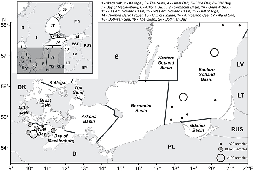
Figure 1. The southern Baltic Sea, with sub-areas according to HELCOM (2016a). The stations included in our calculations are shown as dots of different size and color depending on the sampling frequency.
Methods
The phytoplankton samples were analyzed as described in the manuals of HELCOM (1988, 2014), with standardized biovolume and biomass calculations performed as described by Olenina et al. (2006). For the calculation of the Dia/Dino index, biomass data are inserted into the formula:
where BMDia is the biomass of planktonic diatoms, and BMDino that of autotrophic + mixotrophic dinoflagellates. The index is a simple absolute measure ranging from 0 to 1. Note that the following requirements have to be fulfilled:
1. The Dia/Dino index applies only to the spring bloom. Due to a climatic gradient from the southwest to the northeast Baltic Sea, the timing of the spring bloom differs in the different sub-areas of the sea. We define spring according to the HELCOM definition (HELCOM, 1996), which has been used successfully for many years. Thus, the spring bloom may occur in the period from February to April in the Kattegat/Belt Sea area, including Kiel Bay (cf. Figure 2), and from March to May in the Baltic Proper (see also Carstensen et al., 2004). This period covers also the spring bloom in the northern Baltic Proper (Höglander et al., 2004), Gulf of Finland (Niemi and Ray, 1977; Jaanus and Liiva, 1996), Gulf of Riga (Jurgensone et al., 2011), and the Bothnian Sea (Andersson et al., 1996). In the Bothnian Bay, the spring bloom concept is not directly applicable because the phytoplankton (diatom) growth may start rather late and reaches its peak usually only in June or July (Alasaarela, 1979).
2. Only the autotrophic (including mixotrophs) part of the pelagic community has to be included. Diatoms are always considered as autotrophic, but dinoflagellates may also be mixotrophic or heterotrophic. The mode of nutrition is difficult to identify. Pigmented dinoflagellates are considered as autotrophs but chloroplasts are sometimes hard to recognize. The bloom-forming dinoflagellates present in the spring (Peridiniella catenata, Biecheleria baltica, Gymnodinium corollarium, Scrippsiella hangoei (cf. Klais et al., 2013) are autotrophs. However, the erroneous inclusion of a few doubtful dinoflagellates will not affect the validity of the index. A phytoplankton species list of the Baltic Sea with heterotrophic species marked with an asterisk was compiled by Hällfors (2004). A regularly updated mandatory phytoplankton list is available at the ICES homepage (http://www.ices.dk/marine-data/Documents/ENV/PEG_BVOL.zip). A recent list of diatoms and autotrophic+mixotrophic dinoflagellates of the Baltic Sea is added as Supplementary Material (Table S1).
3. To represent the bloom, one representative sample from the upper mixed layer per sampling date is sufficient, obtained by water sampler, ferry-box, or simply by a bucket. In spring, the upper mixed layer is rather deep and comprises the whole euphotic (trophogenic) layer. Deep chlorophyll maxima, sometimes due to dinoflagellates, rarely occur in spring. Therefore, any depth within the upper mixed layer may be used for sampling, provided that it is really mixed. The influence of time of day is minimal, thus the samples can be taken during the day or night.
4. Only one diatom and dinoflagellate value per season (seasonal mean or maximum) has to be inserted into the formula. Whether mean values over the spring period or simply the peaks of diatom and dinoflagellate biomass best represent the blooms is tested herein (cf. Sections Mean vs. Maximum Value). If the sampling occasions over this period are not evenly distributed, a similar weighting of all phases can be assured by calculating the monthly means as a basis for the calculation of the seasonal mean.
5. The biomass units in the numerator and denominator must be the same. In principle, wet weight or carbon units can be used (Section Wet Weight vs. Carbon Content).
6. If an unusually low Dia/Dino index suggests that the diatom bloom was missed, the potential diatom biomass may be calculated based on silicate consumption [Simax-Simin in μM], as suggested by Wasmund et al. (2013). An alternative Dia/Dino index is then calculated as follows:
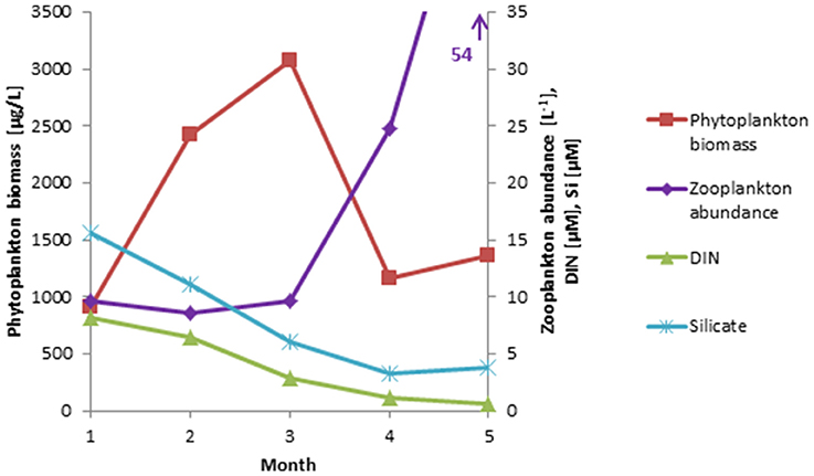
Figure 2. Long-term monthly means (January–May, 2000-2014) of phytoplankton biomass, compared with zooplankton abundance, and nutrient (DIN, Si) concentrations based on recent data (2013-2015) available from Kiel Bay.
Silicate consumption (μM Si) is converted into diatom carbon biomass (μg C/L) using the conversion factors N:Si = 1.25 mol/mol (Sarthou et al., 2005) and C:N = 6.625 (Redfield et al., 1963) and the molar mass of carbon. The combined factor is roughly 100 (1.25*6.625*12.01 = 99.5). If no original carbon data of dinoflagellates are available, their wet weight (BMDino) must be converted into carbon units, using a conversion factor of 0.13 (Edler, 1979). A precondition for this recalculation method is silicate data with sufficient temporal coverage, that is, from the beginning of February to the end of May, to identify the most realistic maxima and minima.
Other silicate-consuming organisms such as Chrysophyceae (e.g., Mallomonas, Synura) originate from freshwater and are rare in the Baltic; thus, they do not affect the calculation of silicate consumption by diatoms. Only the silicoflagellate Dictyocha speculum may form blooms in the western Baltic, but this occurs mostly without a silicon skeleton (Jochem and Babenerd, 1989).
Results
Basic Biomass Data
Combined data from 2000 to 2014 on the seasonal course of the spring bloom in Kiel Bay are shown in Figure 2. The biomass peak may occur in February or March, but the real peak is normally missed by low-frequency sampling. The resulting high variability of the data must be accounted for when calculating and interpreting the Dia/Dino index. In Figure 3, the seasonal maxima of biomasses of diatoms and dinoflagellates during each spring period are shown in one column, but they may occur on different dates. Biomass peak data below a distinct threshold may be due to inadequate sampling and have to be excluded from the analyses. Abnormal Dia/Dino indexes, identified mainly by comparison with the results of the above-described alternative Dia/Dino index, can be excluded most efficiently if a biomass threshold of 1000 μg/L for either diatoms or dinoflagellates was adopted (Figure 3). This threshold demarcated ~25% of the average peak biomass of diatoms plus dinoflagellates over the investigation period. It is valid for the Eastern Gotland Basin and Kiel Bay, but its validity has to be reassessed in other areas. Based on this threshold, the following years had to be excluded from the analysis: 1979, 1980, 1983, 1989, 1990, 1992, 2002, 2006, and 2014 for the Eastern Gotland Basin and 1989, 1992, 1996, 1997, 1998, and 2011 for Kiel Bay. These years are still provisionally shown in Figures 4A, 5A but marked with an “X” to demonstrate the effect of a threshold of 1000 μg/L. Outliers could be removed (Figure 5A) and sub-GES values caused by inadequate sampling are replaced by the more realistic data of the alternative Dia/Dino index for the years 1980, 1983, 1989, 1990, 2002, 2006 and 2014.
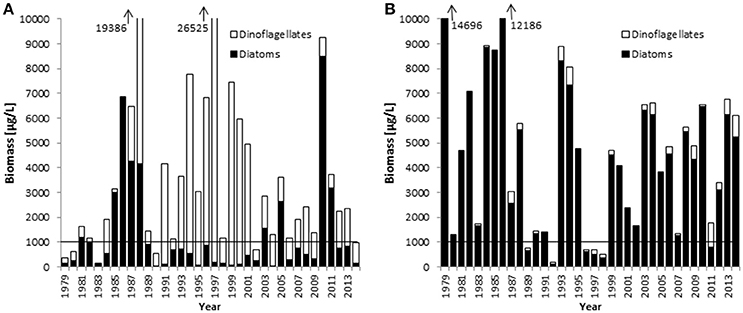
Figure 3. Springtime biomass maxima of diatoms and dinoflagellates between 1979 and 2014 in the Eastern Gotland Basin (A) and Kiel Bay (B). The horizontal lines mark the biomass threshold suggested as the criterion for the applicability of the Dia/Dino index.
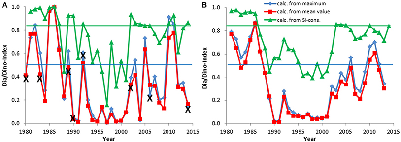
Figure 4. The Dia/Dino index, based on maximum or mean values of wet weight (March–May), and the alternative Dia/Dino index, based on silicate consumption between February and May, in the Eastern Gotland Basin. The indexes are shown for each year (A) and as a moving average over 3 years (B). Years marked with X were excluded from the calculations. The blue line indicates the GES suggested for the standard Dia/Dino index and the red line that for the alternative Dia/Dino index.
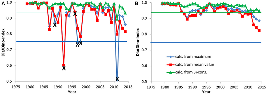
Figure 5. The Dia/Dino index, based on the maximum or mean values of wet weight February-April, and the alternative Dia/Dino index, based on silicate consumption, in Kiel Bay. The indexes are shown for each year (A) and as a moving average over 3 years (B). Years marked with X were excluded from the calculations. The blue line indicates the GES suggested for the standard Dia/Dino index and the red line that for the alternative Dia/Dino index.
Mean vs. Maximum Value
Figures 4A, 5A show examples of the Dia/Dino indexes calculated with the two different procedures: (1) based only on the springtime maxima of diatom and dinoflagellate biomass (wet weight), as shown in blue in the figures, and (2) based on the mean springtime values of diatom and dinoflagellate biomass (wet weight), as shown in red in the figures. Surprisingly, despite the different data basis, the results are similar and the correlation between the two methods is highly significant (Spearman rank correlation ρ = 0.99**).
Wet Weight vs. Carbon Content
In principle, both the wet weight and the carbon content can be used to calculate the Dia/Dino index. A comparison of the two approaches for each sample for which data were available (n = 901) showed that the values of the Dia/Dino index based on wet weight were mostly higher than those based on carbon units (Figure 6).
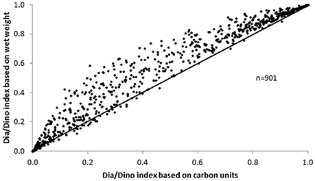
Figure 6. Dia/Dino index based on carbon units vs. wet weight.
Trends of the Dia/Dino Index in Selected Sea Areas
Figure 3 shows that, in the Eastern Gotland Basin, diatom blooms occurred mainly in the 1980s and after the year 2000, whereas dinoflagellates dominated in the 1990s. In Kiel Bay, diatoms dominated the spring bloom, but dinoflagellates increased slightly over the course of the investigation.
The development of the Dia/Dino index over the investigation period is presented in Figures 4, 5. As mentioned in Section Basic Biomass Data, the Dia/Dino indexes of years marked with an “X” are not valid. The strong fluctuations may be smoothed by the use of 3-year moving averages (Figures 4B, 5B), in which each point takes the neighboring years into account and represents the mean of 3 years.
In the open Eastern Gotland Basin (Figure 4A), i.e., excluding the coastal areas, which are influenced by freshwater influxes, the ecosystem shift from the end of the 1980s is well-represented. It shows a decrease from 100% diatom dominance (in 1986) to an almost 0% diatom share (in 1991 and others) compared with dinoflagellates. The smoothed curves (Figure 4B) clearly reveal the low abundance of diatoms from 1990 to 2001, after which diatoms recovered albeit with some fluctuations within this trend.
In Kiel Bay, the Dia/Dino index was high, without any apparent trend (Figure 5A), except between 2012 and 2014, when a slight decrease occurred; this is best seen in the smoothed curve of Figure 5B.
Correlations between the Dia/Dino index and abiotic parameters were checked. Such analyses were already carried through by Wasmund et al. (2013) for the diatom decrease and a connection to the minimum winter temperature was detected. We found a highly significant negative Spearman rank correlation (ρ = −0.48**) between minimum winter temperature and Dia/Dino index in the Eastern Gotland Basin, but not in Kiel Bay.
In Kiel Bay, the potential relationship to zooplankton could be tested because recent zooplankton (size: >100 μm) abundance data were available from three stations of Kiel Bay from 2013 to 2015 (n = 30). These data were compared with long-term phytoplankton biomass data from Kiel Bay for the years 2000–2014 (n = 214) together with data on dissolved inorganic nitrogen (DIN) and silicate. The monthly means of an extended spring period (January to May) are presented in Figure 2, which shows that phytoplankton blooms usually occurred from February to March and then collapsed due to nutrient (DIN) limitation at the end of March, when zooplankton abundance was still low and insufficient to control the diatom bloom.
The Alternative Dia/Dino Index
The trends in the alternative Dia/Dino index, based on silicate consumption, are similar to those determined using the different biomass data (mean and maximum values; Figures 4, 5). The values of the alternative Dia/Dino index, shown in green in the figures, are, however, much higher than those of the standard Dia/Dino index. This is because the alternative Dia/Dino index involves the maximal possible diatom biomass that can grow on the basis of silicate. Accordingly, different GES thresholds have to be defined.
Definition of Good Environmental Status (GES)
The definition of GES is an important precondition for the operationalization of an indicator. Frequently, the most pristine state is considered as defining a GES. Systematically acquired monitoring data have been available in the Baltic Sea only since the 1980s and only these could be used in this paper. However, whether the status of the 1980s is the GES is questionable, because “pristine” conditions in the sea may be those dating back at least to the early twentieth century. Fortunately, high-quality historical quantitative phytoplankton data from the beginning of the twentieth century are available from Kiel Bay and were compiled by Wasmund et al. (2008). Historical Dia/Dino indexes calculated from those data are shown in Table 1. Thus, between 1905 and1950, the historical Dia/Dino index was always >0.87, with a mean value of 0.94. If a deviation of 20% from the historical mean value is tolerated, then a reduction by 0.19 is allowed and the suggested GES threshold will be 0.75. This implies the continued clear dominance of diatoms over dinoflagellates and marks the mid-point between balanced diatom and dinoflagellate biomass (Dia/Dino index = 0.5) and total diatom dominance (Dia/Dino index = 1.0).
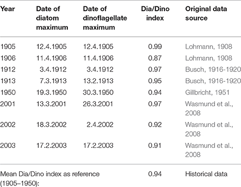
Table 1. The Dia/Dino index, calculated from seasonal carbon biomass peaks, historically and in more recent years, based on data compiled by Wasmund et al. (2008).
For the Eastern Gotland Basin, the reversal point between diatom and dinoflagellate dominance, which occurs at an index value of 0.5, is suggested, with a Dia/Dino index >0.5, i.e., diatom dominance, indicating GES. This is appropriate because the Dia/Dino index covers the whole range from 0 to 1. Based on our suggestions, these GES values have recently been approved by HELCOM (2016b).
As shown in Figures 4, 5, the values of the alternative Dia/Dino index are much higher than those of the standard Dia/Dino index. Consequently, different GES thresholds have to be defined. For this purpose, we compared the standard and the alternative Dia/Dino indexes for each year and tried a linear regression (Figure 7). It was applicable for Kiel Bay (r2 = 0.593), but for the Eastern Gotland Basin, the best correlation was found with a polynomic equation (r2 = 0.588). The correlations between the standard and alternative Dia/Dino indexes are highly significant (p < 0.001). Insertions of the standard GES values into the equations lead to GES values for the alternative Dia/Dino indexes of 0.84 and 0.94 for the Eastern Gotland Basin and Kiel Bay, respectively.
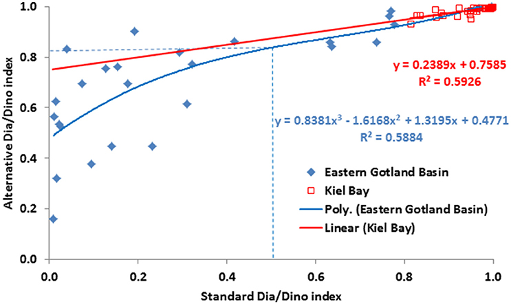
Figure 7. Scatter plot of the standard Dia/Dino (x axis) and alternative Dia/Dino (y axis) indexes and the linear regression between them for Kiel Bay and polynomic regression for the Eastern Gotland Basin. GES values for the Eastern Gotland Basin are shown as broken lines.
Assessments by the standard and alternative Dia/Dino indexes are in good agreement in most cases. Years with a poor GES according to the alternative Dia/Dino index in the Eastern Gotland Basin (1988, 1991, 1993–2001, 2008, 2012) were also identified as “poor” by the standard Dia/Dino index (Figure 4A). The standard Dia/Dino index indicated clearly a worse status than the alternative Dia/Dino index in some years (1984, 2004), probably due to inappropriate sampling, and should not be applied in these exceptional cases (see discussion in Section Restrictions due to Insufficient Biomass Data and Their Potential Rectification). In Kiel Bay, a GES was realized in all years after excluding those marked by “X” (Figure 5A).
Discussion
Restrictions due to Insufficient Biomass Data and Their Potential Rectification
The intensity of a bloom can be characterized by its maximum biomass and duration. These parameters are not accurately recorded by low-frequency routine sampling. However, for this indicator bloom intensity does not require precise quantification; rather, of greater relevance is whether the spring bloom is mainly formed by diatoms or dinoflagellates. For the Dia/Dino index, our results show that, for the specific areas investigated, the spring bloom is sufficiently represented if either diatoms or dinoflagellates reached a biomass threshold of 1000 μg/L. This value turned out to be the best fit to bring the standard Dia/Dino index and the alternative Dia/Dino index into best agreement (Figure 7). In other areas, this threshold may be modified depending on regional conditions.
If this biomass criterion is not met or if otherwise unusually low Dia/Dino indexes were obtained due to inadequate sampling, the alternative Dia/Dino index can be calculated and applied. An example of this latter case was provided by the year 2004 in the Eastern Gotland Basin. As seen in Figure 4A, this year's Dia/Dino index indicates sub-GES but it seems to have been an outlier. In fact, a diatom bloom developed during a large data gap in phytoplankton sampling between 23 March and 22 April 2004, as indicated by a drop in silicate consumption from 13.2 μM (20 March 2004) to 3.6 μM (3 May 2004). In this case, the alternative Dia/Dino index may be applied, which in 2004 yielded a value of 0.85 which still indicates GES.
Mean vs. Maximum Value
If the true peak of the bloom is missed, the approaches based on both the mean and the maximum values are influenced. A calculation based on mean values also takes into account the duration of the bloom. Surprisingly, the two modes of calculation lead to fairly similar Dia/Dino index values.
Diatom blooms are short-lived and disappear quickly whereas dinoflagellate blooms typically last longer (Lips et al., 2014). Therefore, diatoms will be overrated if the calculation is based on maximum values, and dinoflagellates if the calculation is based on mean values. While the two modes of calculation seem to be more or less equivalent, if strict conditions are required then the mean values calculated over the 3-month spring season should be used.
Wet Weight vs. Carbon Content
Abundance and biovolume are determined in microscopic analyses. The conversion of biovolume into biomass (wet weight) is simple, as a constant factor for the density of the cytoplasm is assumed. However, the next step, the conversion from wet weight to carbon, is problematic because it depends on cell size (e.g., Menden-Deuer and Lessard, 2000). As some researchers choose to avoid this vague conversion, carbon biomass is often missing from their data. To utilize the most extensive dataset, we recommend working with the Dia/Dino index based on wet weight, which in most cases will yield higher values than those based on carbon units (Figure 6). This is because wet weight overrates diatoms, as their large vacuole contains only a small amount of carbon but is fully counted in the wet weight. However, especially in spring, when small diatoms dominate, the deviation is small.
Trends in the Dia/Dino Index
The conditions in the different areas of the Baltic Sea are highly diverse, such that trends in the Dia/Dino indexes will differ depending on the sea area (Klais et al., 2011). It is therefore appropriate to adopt the HELCOM sea area structure (Figure 1) as the assessment units for the index and avoid further splitting into sub-areas to prevent reduction of the dataset for each unit.
The trends in the Dia/Dino index in the Eastern Gotland Basin impressively show the ecosystem shift that began at the end of the 1980s, as described by Wasmund et al. (1998) and Alheit et al. (2005). Möllmann et al. (2009) analyzed 52 biotic and abiotic variables in the central Baltic Sea and identified two stable states separated by a transition period lasting from 1988 to 1993. According to Klais et al. (2011), dinoflagellates dominate in the positive phase of the North Atlantic Oscillation (NAO). Our data confirm that the new state of the 1990s persisted for one decade and successively changed back to the earlier state.
In Kiel Bay, the Dia/Dino index was high over the whole period but decreased slightly during the last 3 years of the investigation (Figure 5B). Whether a trend will evolve with the continuation of the data series will be determined with the continued use of the Dia/Dino index. A similar ecosystem shift as in the Baltic Proper might also occur in the western Baltic Sea. In that case, the recent situation provides a baseline for identifying future changes in the ecosystem almost in real-time.
Indicator of Food Web Changes
Identification of the reasons for the long-term changes in the Dia/Dino index may help to understand its ecological relevance. Wasmund et al. (2013) showed that diatom spring blooms were strong after cold winters in the Eastern Gotland Basin but not in Kiel Bay. Therefore, it was not surprising that we found a highly significant negative correlation between minimum winter temperature and Dia/Dino index for the Eastern Gotland Basin.
Wasmund et al. (2013) argued that the reduction in diatoms after mild winters cannot be caused by a direct physiological effect of a slight temperature change, but by temperature-sensitive hydrographical (bottom-up) or biological (top-down) impacts that respond strongly to moderate temperature changes. They discussed two hypotheses: (i) a lack of convective mixing after mild winters may inhibit diatom growth, and (ii) a higher overwintering zooplankton biomass could graze on the early diatom blooms.
We favor the latter, food-web hypothesis: Zooplankton growth is earlier and stronger after mild winters, when these organisms feed on the diatom bloom, whereas it occurs later and is unable to control the diatom bloom after cold winters (see references in Wasmund et al., 2013). In their study of sediments from the Bornholm Basin, Dutz et al. (2004) found high hatching rates of nauplii already in March and April, with strong increases in those rates as the incubation temperature increased. In mesocosm experiments, warming led to a reduced time-lag between the phytoplankton bloom and the microzooplankton biomass maximum (Horn et al., 2015). Therefore, early diatoms can be controlled by grazing, which implies lower and later algal peaks at higher temperatures (Gaedke et al., 2010).
If a diatom bloom fails, the persisting nutrients enhance dinoflagellate growth, resulting in a prolongation of the spring bloom, a delay and reduction in sedimentation, and the prolonged persistence of suspended material in the pelagial (Heiskanen, 1998; Tamelander and Heiskanen, 2004). This sequence of events will be manifested as a better temporal match between the spring bloom and developing copepods and as an intensified microbial food web, as more nutrients remain in the mixed surface layer after stratification of the water column (Heiskanen, 1998).
This mechanism does not occur in small and shallow Kiel Bay, where the spring bloom develops early, irrespective of the temperature, while zooplankton develops in April and is thus unable to control the diatom spring bloom because of a mismatch in their occurrences (Smetacek, 1985). This scenario was confirmed by results presented in Section Trends of the Dia/Dino Index in Selected Sea Areas (Figure 2).
Not only grazing by zooplankton but also infections by parasites may control the diatom blooms in the Baltic Proper. Diatoms are a preferred host for fungal parasites in spring (Gutiérrez et al., 2016). Peacock et al. (2014) found abundant infesting stages of parasites only at water temperatures >4°C. Therefore, diatoms are not only subject to zooplankton grazing but also to infections especially after mild winters. They survive better in colder waters. This observation provides strong support for our food-web hypothesis.
The typical diatom spring bloom grows rapidly in response to new nutrients, but when the supply of the limiting nutrient is exhausted, the diatoms starve and quickly sink without significant decomposition (von Bodungen, et al., 1981; Tallberg and Heiskanen, 1998). At this stage they provide food to the benthos, which leads to enhanced metabolic activities in the sediment (Graf et al., 1982) and to the growth of suspension-feeding bivalves (own data, not shown). The resulting stimulation of the natural purification processes of the Baltic Sea is an important ecosystem service provided by these organisms (Karlson et al., 2007).
The effect of a stronger sedimentation will depend on the region. Particles that sink to oxic bottom areas feed the benthos, whereas those that reach deep anoxic basins devoid of zoobenthos will be subject to anaerobic bacterial degradation processes, leading to a stronger oxygen deficit (Spilling and Lindström, 2008). The effects of oxygen deficit will be discussed in Section Indicator of Eutrophication.
Whether diatoms or dinoflagellates are the most desirable food depends on different factors. Representatives of both groups may be appropriate as food, but those that are toxic must obviously be avoided and those that are of reduced nutritional quality, mucus-producing, or covered by thick cell walls are undesirable (Mitra and Flynn, 2005).
Traditionally, diatoms were considered the most important primary food source in the marine food web, and dinoflagellates of only minor importance (Kleppel, 1993; Turner, 1997). For example, in the southern Benguela upwelling system, egg production by adult female copepods was higher in waters dominated by diatoms than by microflagellates (Walker and Peterson, 1991). Recently, low food quality of diatoms (Ask et al., 2006; Dutz et al., 2008; Koski et al., 2008) and the inhibitory effects of this group of organisms (Turner et al., 2001; Ianora et al., 2003; Barreiro et al., 2011) have also been described, leading Uusitalo et al. (2013) to conclude that diatoms can generally be considered as poor-quality food. According to Vehmaa et al. (2012), however, a food-quality approach based on class level is too simplistic; rather, phytoplankton taxa must be considered at the species level.
Within our study we could not resolve the question of food quality. Therefore, we regarded for the Dia/Dino index primarily the aspect of vertical mass transport and considered it as an indicator of the food pathway. A high Dia/Dino index indicates stronger sedimentation and therefore a better nutrition of the benthos, and a low Dia/Dino index a better nutrition of the pelagic components of the food web.
In case of doubt whether diatoms or dinoflagellates are more beneficial for the ecosystem, the most pristine state is considered as GES. We were able to use historical data from Kiel Bay to define the GES there (Table 1). The suggestions of GES thresholds were carefully checked by HELCOM expert teams and confirmed to be reasonable by an intensive study of historical data by Wasmund (2017).
Indicator of Eutrophication
Besides the food web hypothesis as a possible explanation for the temporal decrease in diatoms, their limitation by silicate might be contemplated based on the long-term decrease in silicate concentrations in the Baltic Sea over the last 40 or even 100 years (Papush and Danielsson, 2006; Conley et al., 2008). At present, this hypothesis can be rejected, as during a 30-year period there has been no trend in silicate concentrations in the Baltic Proper (Wasmund et al., 2013). The silicate concentrations after the winter fluctuated between 10 and 25 μmol/L and were high enough to support the formation of a diatom bloom.
Silicate is currently not of concern because nitrogen and phosphorus are the drivers of eutrophication. However, with ongoing input of nitrogen and phosphorus, the relative concentration of silicate will decrease such that silicate may become the limiting nutrient for diatom growth (Danielsson et al., 2008; Ferreira et al., 2011). Indeed, in the 1980s, silicate was nearly depleted by the spring blooms in the Baltic Proper (Wasmund et al., 2013). Therefore, the Dia/Dino index will decrease with eutrophication and a high Dia/Dino index will indicate a less eutrophied status.
Strong diatom blooms, i.e., high Dia/Dino indexes, may help mitigating eutrophication as they remove nutrients by intensive sedimentation and deposit them in the sediment. Moreover, mediated by higher sedimentation rates, water transparency increases which is beneficial for the phytobenthos in the shallow areas. However, high rates of sedimentation have negative effects on the oxygen regime and connected processes in the deep basins of the Baltic. Under reducing chemical conditions nutrients are released from the sediment and may enhance eutrophication (Conley et al., 2002; Karlson et al., 2007). Anoxic areas cover, however, only a small part of the total Baltic area recently (Feistel et al., 2016). Borders between oxic and anoxic regions are not visible in the sea's intermediate and upper layers because of intensive transport and mixing processes. Therefore, we do not differentiate between oxic and anoxic regions for assessments based on the Dia/Dino index, which examines only the upper water layer. We assume that the comparably large oxic areas have the greater impact.
A summary of the main effects of a high Dia/Dino index on an ecosystem is given in Table 2.
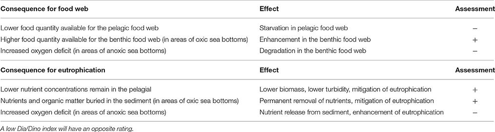
Table 2. Consequences and resulting effects of a high Dia/Dino index on an ecosystem and the assessment whether it is positive (+) or negative (−) for the ecological status.
Limitations and Advantages of the Dia/Dino Index
Limitations caused by undersampling are general phenomena connected with field data. Inadequate data caused by missing the diatom blooms may be excluded by a biomass threshold that has to be reached; they may be replaced by silicate consumption data which allow the calculation of an alternative Dia/Dino index. These limitations and potential rectification are extensively discussed above.
The Dia/Dino index is not applicable in areas where diatoms or dinoflagellates do not occur for natural reasons. Diatoms can generally grow throughout the Baltic Sea, but dinoflagellates are restricted to marine and brackish waters. Therefore, the Dia/Dino index is not applicable in freshwater-influenced areas such as lagoons (Olenina, 1998; Gasiūnaitė et al., 2005), large river plumes (Wasmund et al., 1999), and parts of the Gulf of Bothnia (Klais et al., 2011).
The validity of the Dia/Dino index may be reduced if other phytoplankton groups gain dominance in spring. In the Baltic Proper, the mixotrophic ciliate Mesodinium rubrum may become the dominant species in spring (Wasmund and Siegel, 2008; van Beusekom et al., 2009), and in Kiel Bay dictyochophyceae may compete with dinoflagellates. To keep the indicator simple and common for the whole Baltic area, other, sporadically dominating algal groups have been excluded from the assessment protocol.
This indicator is robust, as it is based on only two groups that can be identified easily, even without extensive taxonomic expertise, on the basis of approved routine methods. It reflects a wide range of naturally occurring changes, by covering the whole theoretically possible range in values from 0 to 1. The calculation is simple and traceable, and the necessary data can be acquired from existing monitoring programs. Phytoplankton data have been collected for many years in the COMBINE monitoring program of HELCOM and diverse national monitoring programs and are stored in accessible data banks, e.g., the COMBINE database hosted at the International Council for the Exploration of the Sea (ICES: http://dome.ices.dk/views/Phytoplankton.aspx).
As anthropogenic activities have only an indirect effect on the ratio of diatoms and dinoflagellates, the Dia/Dino index cannot be readily manipulated, except for cases of severe eutrophication that may lead to silicate limitation. It serves primarily as a descriptive trend indicator.
Summary
Use of the Dia/Dino index is recommended based on the following requirements:
1. A specific sampling technique is not required. A representative sample from the upper mixed layer obtained by water sampler, ferry-box, or simply by a bucket is sufficient.
2. Biomass (wet weight) data of diatoms and autotrophic+mixotrophic dinoflagellates should be determined using an inverted microscope according to compulsory monitoring guidelines (HELCOM, 2014).
3. Only the spring season, i.e., from February to April in the Kattegat/Belt Sea area and from March to May in the Baltic Proper, has to be considered.
4. Seasonal mean values of diatoms and dinoflagellates must be calculated and used to calculate the index. If the sampling data are not evenly distributed over the season, monthly means must be calculated first, as a basis for the seasonal means. To strengthen the data, the assessment area should be represented by several stations.
5. The spring data must be checked for the maximum biomass values of diatoms and dinoflagellates. If one of these values exceeds a threshold, e.g., 1000 μg/L in the areas investigated, the data may be used. For other regions, the value of this threshold has to be adjusted according to the specific conditions.
6. If an unusually low Dia/Dino index is obtained because of missing diatom blooms, an alternative Dia/Dino index can be calculated by replacing the diatom biomass with silicate consumption values and the subsequent application of conversion factors according to Wasmund et al. (2013).
7. For the two examples considered, GES thresholds of 0.75 for Kiel Bay and 0.5 for the Eastern Gotland Basin were suggested and finally approved by HELCOM (2016b). Values exceeding this threshold are considered as indicative of GES. If the alternative Dia/Dino index is applied, GES thresholds of 0.94 for Kiel Bay and 0.84 for the Eastern Gotland Basin are recommended.
A high Dia/Dino index is assumed to be an indicator of good environmental conditions. Because of intense diatom sedimentation, a high index value is related to high-level food delivery to the benthos but low food availability to zooplankton and therefore to a lower trophic state in the pelagial. The index provides information for Descriptor 4 (food web) of the MSFD. A reduced Dia/Dino index may also indicate silicate limitation owing to severe eutrophication, which is linked to high nitrogen and phosphorus but not silicate inputs (Descriptor 5 of the MSFD).
Indicators focus on only one or a few key components of the ecosystem. For a complex assessment of the state of the ecosystem, an entire suite of the various indicators has to be combined. For example, for fully quantitative information, the Dia/Dino index could be connected with other indicators such as chlorophyll a. The combination of the different indicators to obtain a holistic view is beyond the scope of this paper but is planned in the Holistic Assessment by HELCOM in 2018.
Author Contributions
NW developed the idea of this indicator and initiated a discussion forum, compiled the data of the other contributors and carried through first calculations; he was the main writer of the paper. JK, JG, AJ, MJ, IJ, and SL are contributors of the basic data used; they participated in the discussion forum and were involved in writing the paper. MP was engaged in a German research project for management of the data of the western Baltic Sea, which were included in this paper.
Conflict of Interest Statement
Parts of the work (Kiel Bay data processing) were parts of a research project supported by Bundesamt für Naturschutz (BfN), with funds from the German Bundesministerium für Umwelt, Naturschutz, Bau, und Reaktorsicherheit. The evaluation of data from the southern part of the Eastern Gotland was supported by statutory activity of the National Marine Fisheries Research Institutes (NMFRI) and by Polish National Environmental Monitoring (PMŚ). The funding agencies have never exert influence on our work and the conclusions.
The authors declare that the research was conducted in the absence of any commercial or financial relationships that could be construed as a potential conflict of interest.
Acknowledgments
Discussions on the Dia/Dino index as a potential indicator were stimulated by projects of HELCOM, particularly the “Operationalization of HELCOM core indicators” (CORESET II) and the Phytoplankton Expert Group (PEG). Evaluation of the Kiel Bay data was supported by Bundesamt für Naturschutz (BfN), with funds from the German Bundesministerium für Umwelt, Naturschutz, Bau und Reaktorsicherheit (Grant Z1.2-53202/2015/5). The evaluation of data from the southern part of the Eastern Gotland Basin was supported by statutory activity of the National Marine Fisheries Research Institutes (NMFRI) and by Polish National Environmental Monitoring (PMŚ).
Supplementary Material
The Supplementary Material for this article can be found online at: https://www.frontiersin.org/article/10.3389/fmars.2017.00022/full#supplementary-material
Table S1. List of planktonic autotrophic+mixotrophic as well as heterotrophic dinoflagellates and diatoms of the Baltic Sea, extracted from the current file PEG_BVOL2016 available at http://www.ices.dk/marine-data/Documents/ENV/PEG_BVOL.zip. Also higher taxonomic levels (as for example Gymnodiniales, Peridiniales, Centrales, Pennales) are included because not all objects can be identified on the species level. Some of the higher taxa can have both autotrophic and heterotrophic members (e.g., Amphidinium sp., Glenodinium sp., Gymnodiniales, Gymnodinium sp., Gyrodinium sp., Katodinium sp., Peridiniales). Also author epithet for the species is given.
References
Alasaarela, E. (1979). Phytoplankton and environmental conditions in central and coastal areas of the Bothnian Bay. Ann. Bot. Fennici 16, 241–274.
Alheit, J., Möllmann, C., Dutz, J., Kornilovs, G., Loewe, P., Mohrholz, V., et al. (2005). Synchronous ecological regime shifts in the central Baltic and the North Sea in the late 1980s. ICES J. Mar. Sci. 62, 1205–1215. doi: 10.1016/j.icesjms.2005.04.024
Andersen, J. H., Aroviita, J., Carstensen, J., Friberg, N., Johnson, R. K., Kauppila, P., et al. (2016). Approaches for integrated assessment of ecological and eutrophication status of surface waters in Nordic Countries. Ambio 45, 681–691. doi: 10.1007/s13280-016-0767-8
Andersson, A., Hajdu, S., Haecky, P., Kuparinen, J., and Wikner, J. (1996). Succession and growth limitation of phytoplankton in the Gulf of Bothnia (Baltic Sea). Mar. Biol. 126, 791–801. doi: 10.1007/BF00351346
Ask, J., Reinikainen, M., and Bamstedt, U. (2006). Variation in hatching success and egg production of Eurytemora affinis (Calanoida, Copepoda) from the Gulf of Bothnia, Baltic Sea, in relation to abundance and clonal differences of diatoms. J. Plankton Res. 28, 683–694. doi: 10.1093/plankt/fbl005
Barreiro, A., Carotenuto, Y., Lamari, N., Esposito, F., D'Ippolito, G., Fontana, A., et al. (2011). Diatom induction of reproductive failure in copepods: the effect of PUAs versus non volatile oxylipins. J. Exp. Mar. Biol. Ecol. 401, 13–19. doi: 10.1016/j.jembe.2011.03.007
Beaugrand, G., Harlay, X., and Edwards, M. (2014). Detecting plankton shifts in the North Sea: a new abrupt ecosystem shift between 1996 and 2003. Mar. Ecol. Prog. Ser. 502, 85–104. doi: 10.3354/meps10693
Borja, A., Elliott, M., Andersen, J. H., Berg, T., Carstensen, J., Halpern, B. S., et al. (2016). Overview of integrative assessment of marine systems: the ecosystem approach in practice. Front. Mar. Sci. 3, 1–20. doi: 10.3389/fmars.2016.00020
Borja, A., Elliott, M., Andersen, J. H., Cardoso, A. C., Carstensen, J., Ferreira, J. G., et al. (2013). Good environmental status of marine ecosystems: what is it and how do we know when we have attained it? Mar. Pollut. Bull. 76, 16–27. doi: 10.1016/j.marpolbul.2013.08.042
Borja, A., Prins, T. C., Simboura, N., Andersen, J. H., Berg, T., Marques, J.-C., et al. (2014). Tales from a thousand and one ways to integrate marine ecosystem components when assessing the environmental status. Front. Mar. Sci. 1, 1–20. doi: 10.3389/fmars.2014.00072
Bralewska, J. M. (1992). “Cyclic seasonal fluctuations of the phytoplankton biomass and composition in the Gdansk Basin in 1987-1988,” in ICES Council Meeting/L:15 (Rostock-Warnemünde), 1–40. Available online at: http://www.ices.dk/sites/pub/CM%20Doccuments/1992/L/1992_L15.pdf
Busch, W. (1916-1920). Über das Plankton der Kieler Föhrde im Jahre 1912/13. Wissenschaftliche Meeresuntersuchungen, Neue Folge: Abt. Kiel. 25–142.
Carstensen, J., Helminen, U., and Heiskanen, A.-S. (2004). Typology as a structuring mechanism for phytoplankton composition in the Baltic Sea. Coastline Rep. 4, 55–64. Available online at: http://databases.eucc-d.de/files/documents/00000311_no5_carstensen.pdf
Conley, D., Humborg, C., Rahm, L., Savchuk, O. P., and Wulff, F. (2002). Hypoxia in the Baltic Sea and basin-scale changes in phosphorus biogeochemistry. Environ. Sci. Technol. 36, 5315–5320. doi: 10.1021/es025763w
Conley, D. J., Humborg, C., Smedberg, E., Rahm, L., Papush, L., Danielsson, A., et al. (2008). Past, present and future state of the biogeochemical Si cycle in the Baltic Sea. J. Mar. Syst. 73, 338–346. doi: 10.1016/j.jmarsys.2007.10.016
Danielsson, A., Papush, L., and Rahm, L. (2008). Alterations in nutrient limitations - scenarios of a changing Baltic Sea. J. Mar. Syst. 73, 263–283. doi: 10.1016/j.jmarsys.2007.10.015
Dutz, J., Koski, M., and Jónasdóttir, S. H. (2008). Copepod reproduction is unaffected by diatom aldehydes or lipid composition. Limnol. Oceanogr. 53, 225–235. doi: 10.4319/lo.2008.53.1.0225
Dutz, J., Mohrholz, V., Peters, J., Renz, J., and Alheit, J. (2004). “Identification of critical stages in the population dynamics of key copepod species in the Bornholm Basin (Baltic Sea): potential linkages to physical forcing and climate variability,” in ICES Conference Meeting 2004/L:12 (Copenhagen), 1–11. Available online at: http://www.ices.dk/sites/pub/CM%20Doccuments/2004/L/L1204.pdf
Edler, L. (ed.). (1979). “Recommendations on methods for marine biological studies in the Baltic Sea,” in Phytoplankton and Chlorophyll (Malmö: The Baltic Marine Biologists), 1–38.
European Commission (2008). Directive 2008/56/EC of the European Parliament and of the council of 17 June 2008, establishing a framework for community action in the field of marine environmental policy (Marine Strategy Framework Directive). Official J. Eur. Union L 164, 19–40. Available online at: http://eur-lex.europa.eu/legal-content/EN/TXT/PDF/?uri=CELEX:32008L0056&rid=1
Feistel, S., Feistel, R., Nehring, D., Matthäus, W., Nausch, G., and Naumann, M. (2016). Hypoxic and anoxic regions in the Baltic Sea, 1969-2015. Meereswiss. Ber. Warnemünde 100, 1–84. doi: 10.12754/msr-2016-0100
Ferreira, J. G., Andersen, J. H., Borja, A., Bricker, S. B., Camp, J., Cardoso da Silva, M., et al. (2011). Overview of eutrophication indicators to assess environmental status within the European Marine Strategy Framework Directive. Estuar. Coast. Shelf Sci. 93, 117–131. doi: 10.1016/j.ecss.2011.03.014
Gaedke, U., Ruhenstroth-Bauer, M., Wiegand, I., Tirok, K., Aberle, N., Breithaupt, P., et al. (2010). Biotic interactions may overrule direct climate effects on spring phytoplankton dynamics. Glob. Chang. Biol. 16, 1122–1136. doi: 10.1111/j.1365-2486.2009.02009.x
Gasiūnaitė, Z. R., Cardoso, A. C., Heiskanen, A.-S., Henriksen, P., Kauppila, P., Olenina, I., et al. (2005). Seasonality of coastal phytoplankton in the Baltic Sea: influence of salinity and eutrophication. Estuar. Coast. Shelf Sci. 65, 239–252. doi: 10.1016/j.ecss.2005.05.018
Gillbricht, M. (1951). Produktionsbiologische Untersuchungen in der Kieler Bucht. Ph.D. thesis, Univ. Kiel.
Graf, G., Bengtsson, W., Diesner, U., and Schulz, R. (1982). Benthic response to sedimentation of a spring phytoplankton bloom: process and budget. Mar. Biol. 67, 201–208. doi: 10.1007/BF00401286
Gutiérrez, M. H., Jara, A. M., and Pantoja, S. (2016). Fungal parasites infect marine diatoms in the upwelling ecosystem of the Humboldt current system off central Chile. Environ. Microbiol. 18, 1646–1653. doi: 10.1111/1462-2920.13257
Hällfors, G. (2004). “Checklist of Baltic Sea Phytoplankton Species including some heterotrophic protistan groups,” in Baltic Sea Environment Proceedings, 1–208. Available online at: http://www.helcom.fi/Lists/Publications/BSEP95.pdf.
Heiskanen, A.-S. (1998). Factors governing sedimentation and pelagic nutrient cycles in the northern Baltic Sea. Monogr. Boreal Environ. Res. 8, 1–80.
HELCOM (1988). Guidelines for the baltic monitoring programme for the third stage. Part D. biological determinands. Baltic Sea Environ. Proc. 27 D, 1–161.
HELCOM (1996). Third periodic assessment of the state of the marine environment of the Baltic Sea, 1989-1993; background document. Baltic Sea Environ. Proc. 64 B, 252.
HELCOM (2010). Ecosystem health of the Baltic Sea 2003–2007. HELCOM initial holistic assessment. Baltic Sea Environ. Proc. 122, 1–68.
HELCOM (2013). HELCOM core indicators. Final report of the HELCOM CORESET project. Baltic Sea Environ. Proc. 136, 1–74.
HELCOM (2014). Manual for Marine Monitoring in the COMBINE Programme of HELCOM. Available online at: http://www.helcom.fi/Documents/Action%20areas/Monitoring%20and%20assessment/Manuals%20and%20Guidelines/Manual%20for%20Marine%20Monitoring%20in%20the%20COMBINE%20Programme%20of%20HELCOM.pdf
HELCOM (2015). Outcome of the Second Meeting of the Working Group on the State of the Environment and Nature Conservation (State & Conservation 2-2015). Available online at: https://portal.helcom.fi/meetings/STATE-CONSERVATION%202-2015-232/MeetingDocuments/Outcome%20of%20STATE-CONSERVATION%202-2015.pdf
HELCOM (2016a): Baltic Sea environmental Status Map Service. Available online at: http://maps.helcom.fi/website/SeaEnvironmentalStatus/index.html
HELCOM (2016b). Outcome of the Fifth Meeting of the Working Group on the State of the Environment and Nature Conservation (State & Conservation 5-2016). Available online at: https://portal.helcom.fi/meetings/STATE%20-%20CONSERVATION%205-2016-363/MeetingDocuments/Final%20Outcome%20State%20and%20Conservation%205-2016.pdf
Höglander, H., Karlson, B., Johansen, M., Walve, J., and Andersson, A. (2013). Overview of Coastal Phytoplankton Indicators and their Potential Use in Swedish Waters. Havsmiljöinstitutet. Available online at: http://www.waters.gu.se/rapporter
Höglander, H., Larsson, U., and Hajdu, S. (2004). Vertical distribution and settling of spring phytoplankton in the offshore NW Baltic Sea proper. Mar. Ecol. Prog. Ser. 283, 15–27. doi: 10.3354/meps283015
Horn, H. G., Boersma, M., Garzke, J., Löder, M. G. J., Sommer, U., and Aberle, N. (2015). Effects of high CO2 and warming on a Baltic Sea microzooplankton community. ICES J. Mar. Sci. 73, 772–782. doi: 10.1093/icesjms/fsv198
Ianora, A., Poulet, S. A., and Miralto, A. (2003). The effect of diatoms on copepod reproduction: a review. Phycologia 42, 351–363. doi: 10.2216/i0031-8884-42-4-351.1
Jaanus, A., and Liiva, K. (1996). A review of the phytoplankton monitoring data in the southern Gulf of Finland and an attempt at biogeographical grouping on these grounds. Proc. Estonian Acad. Sci. Ecol. 6, 57–72.
Jochem, F., and Babenerd, B. (1989). Naked Dictyocha speculum - a new type of phytoplankton bloom in the western Baltic. Mar. Biol. 103, 373–379. doi: 10.1007/BF00397272
Jurgensone, I., Carstensen, J., Ikainiece, A., and Kalveka, B. (2011). Long-term changes and controlling factors of phytoplankton community in the Gulf of Riga (Baltic Sea). Estuaries Coasts 34, 1205–1219. doi: 10.1007/s12237-011-9402-x
Karlson, K., Bonsdorff, E., and Rosenberg, R. (2007). The impact of benthic macrofauna for nutrient fluxes from Baltic Sea sediments. Ambio 36, 161–167. doi: 10.1579/0044-7447(2007)36[161:TIOBMF]2.0.CO;2
Klais, R., Tamminen, T., Kremp, A., Spilling, K., An, B. W., Hajdu, S., et al. (2013). Spring phytoplankton communities shaped by interannual weather variability and dispersal limitation: mechanisms of climate change effects on key coastal primary producers. Limnol. Oceanogr. 58, 753–762. doi: 10.4319/lo.2013.58.2.0753
Klais, R., Tamminen, T., Kremp, A., Spilling, K., and Olli, K. (2011). Decadal-scale changes of dinoflagellates and diatoms in the anomalous Baltic sea spring bloom. PLoS ONE 6:e21567. doi: 10.1371/journal.pone.0021567
Kleppel, G. S. (1993). On the diets of the calanoid copepods. Mar. Ecol. Prog. Ser. 99, 183–195. doi: 10.3354/meps099183
Koski, M., Wichard, T., and Jónasdóttir, S. H. (2008). “Good” and “bad” diatoms: development, growth and juvenile mortality of the copepod Temora longicornis on diatom diets. Mar. Biol. 154, 719–734. doi: 10.1007/s00227-008-0965-4
Kraberg, A. C., Wasmund, N., Vanaverbeke, J., Schiedek, D., Wiltshire, K. H., and Mieszkowska, N. (2011). Regime shifts in the marine environment: the scientific basis and political context. Mar. Pollut. Bull. 62, 7–20. doi: 10.1016/j.marpolbul.2010.09.010
Lips, I., Rünk, N., Kikas, V., Meerits, A., and Lips, U. (2014). High-resolution dynamics of the spring bloom in the Gulf of Finland of the Baltic Sea. J. Mar. Syst. 129, 135–149. doi: 10.1016/j.jmarsys.2013.06.002
Lohmann, H. (1908). Untersuchungen zur Feststellung des vollständigen Gehaltes des Meeres an Plankton. Wiss. Meeresuntersuchungen Kiel N. F. 10, 130–370.
Menden-Deuer, S., and Lessard, E. J. (2000). Carbon to volume relationsships for dinoflagellates, diatoms and other protist plankton. Limnol. Oceanogr. 45, 569–579. doi: 10.4319/lo.2000.45.3.0569
Mitra, A., and Flynn, K. J. (2005). Predator-prey interactions: is “ecological stoichiometry” sufficient when good food goes bad? J. Plankton Res. 27, 393–399. doi: 10.1093/plankt/fbi022
Möllmann, C., Diekmann, R., Müller-Karulis, B., Kornilovs, G., Plikshs, M., and Axe, P. (2009). The reorganization of a large marine ecosystem due to atmospheric and anthropogenic pressure - a discontinuous regime shift in the central Baltic Sea. Glob. Change. Biol. 15, 1377–1393. doi: 10.1111/j.1365-2486.2008.01814.x
Niemi, Å., and Ray, I.-L. (1977). Phytoplankton production in Finnish coastal waters. Report 2: phytoplankton biomass and composition in 1973. MERI 4, 6–22.
Olenina, I. (1998). Long-term changes in the Kursiu Marios lagoon: eutrophication and phytoplankton response. Ekologija 1, 56–65.
Olenina, I., Hajdu, S., Andersson, A., Edler, L., Wasmund, N., Busch, S., et al. (2006). “Biovolumes and size-classes of phytoplankton in the Baltic Sea,” in Baltic Sea Environment Proceedings, 144. Available online at: http://www.helcom.fi/Lists/Publications/BSEP106.pdf
Papush, L., and Danielsson, A. (2006). Silicon in the marine environment: dissolved silica trends in the Baltic Sea. Estuar. Coast. Shelf Sci. 67, 53–66. doi: 10.1016/j.ecss.2005.09.017
Peacock, E. E., Olson, R. J., and Sosik, H. M. (2014). Parasitic infection of the diatom Guinardia delicatula, a recurrent and ecologically important phenomenon on the New England Shelf. Mar. Ecol. Prog. Ser. 503, 1–10. doi: 10.3354/meps10784
Redfield, A. C., Ketchum, B. H., and Richards, F. A. (1963). “The influence of organisms on the composition of seawater,” in The Sea, ed M. N. Hill (New York, NY: Wiley), 26–77.
Sarthou, G., Timmermans, K. R., Blain, S., and Tréguer, P. (2005). Growth physiology and fate of diatoms in the ocean: a review. J. Sea Res. 53, 25–42. doi: 10.1016/j.seares.2004.01.007
Smayda, T. J., and Reynolds, C. S. (2001). Community assembly in marine phytoplankton: application of recent models to harmful dinoflagellate blooms. J. Plankton Res. 23, 447–461. doi: 10.1093/plankt/23.5.447
Smetacek, V. (1985). The annual cycle of Kiel Bight plankton: a long-term analysis. Estuaries 8, 145–157. doi: 10.2307/1351864
Smetacek, V. (1999). Diatoms and the ocean carbon cycle. Protist 150, 25–32. doi: 10.1016/S1434-4610(99)70006-4
Spilling, K., Kremp, A., Klais, R., Olli, K., and Tamminen, T. (2014). Spring bloom community change modifies carbon pathways and C:N:P:Chl a stoichiometry of coastal material fluxes. Biogeosci. Discuss. 11, 7275–7289. doi: 10.5194/bg-11-7275-2014
Spilling, K., and Lindström, M. (2008). Phytoplankton life cycle transformations lead to species-specific effects on sediment processes in the Baltic Sea. Cont. Shelf Res. 17, 2488–2495. doi: 10.1016/j.csr.2008.07.004
Spilling, K., and Markager, S. (2008). Ecophysiological growth characteristics and modelling of the onset of the spring bloom in the Baltic Sea. J. Mar. Syst. 73, 323–337. doi: 10.1016/j.jmarsys.2006.10.012
Tallberg, P., and Heiskanen, A.-S. (1998). Species-specific phytoplankton sedimentation in relation to primary production along an inshore-offshore gradient in the Baltic Sea. J. Plankton Res. 20, 2053–2070. doi: 10.1093/plankt/20.11.2053
Tamelander, T., and Heiskanen, A.-S. (2004). Effects of spring bloom phytoplankton dynamics and hydrography on the composition of settling material in the coastal northern Baltic Sea. J. Mar. Res. 52, 217–234. doi: 10.1016/j.jmarsys.2004.02.001
Teixeira, H., Berg, T., Uusitalo, L., Fürhaupter, K., Heiskanen, A.-S., Mazik, K., et al. (2016). A catalogue of marine biodiversity indicators. Front. Mar. Sci. 3:207. doi: 10.3389/fmars.2016.00207
Turner, J. T. (1997). Toxic marine phytoplankton, zooplankton grazers, and pelagic food webs. Limnol. Oceanogr. 42, 1203–1214. doi: 10.4319/lo.1997.42.5_part_2.1203
Turner, J. T., Ianora, A., Miralto, A., Laabir, M., and Esposito, F. (2001). Decoupling of copepod grazing rates, fecundity and egg-hatching success on mixed and alternating diatom and dinoflagellate diets. Mar. Ecol. Prog. Ser. 220, 187–199. doi: 10.3354/meps220187
Uusitalo, L., Hällfors, H., Peltonen, H., Kiljunen, M., Jounela, P., and Aro, E. (2013). “Indicators of the Good Environmental Status of Food Webs in the Baltic Sea” (GES-REG project report). Available online at: http://projects.centralbaltic.eu/images/files/result_pdf/GESREG_result3_Food_webs_report_ENG.pdf
van Beusekom, J. E. E., Mengedoht, D., Augustin, C. B., Schilling, M., and Boersma, M. (2009). Phytoplankton, protozooplankton and nutrient dynamics in the Bornholm Basin (Baltic Sea) in 2002-2003 during the German GLOBEC Project. Int. J. Earth Sci. Geol. Rundsch. 98, 251–260. doi: 10.1007/s00531-007-0231-x
Vehmaa, A., Kremp, A., Tamminen, T., Hogfors, H., Spilling, K., and Engström-Öst, J. (2012). Copepod reproductive success in spring-bloom communities with modified diatom and dinoflagellate dominance. ICES J. Mar. Sci. 69, 351–357. doi: 10.1093/icesjms/fsr138
von Bodungen, B., von Bröckel, K., Smetacek, V., and Zeitzschel, B. (1981). Growth and sedimentation of the phytoplankton spring bloom in the Bornholm Sea (Baltic Sea). Kieler Meeresforsch. Sonderh. 5, 49–60.
Walker, D. R., and Peterson, W. T. (1991). Relationships between hydrography, phytoplankton production, biomass, cell size and species composition, and copepod production in the southern Benguela upwelling system in April 1988. S. Afr. J. Mar. Sci. 11, 289–305. doi: 10.2989/025776191784287529
Wasmund, N. (2017). The diatom/dinoflagellate index as an indicator of ecosystem changes in the Baltic Sea. 2. Historical data as criterion for the good environmental status. Front. Mar. Sci. 4:22. doi: 10.3389/fmars.2017.00022
Wasmund, N., Göbel, J., and Bodungen, B. V. (2008). 100-years-changes in the phytoplankton community of Kiel Bight (Baltic Sea). J. Mar. Syst. 73, 300–322. doi: 10.1016/j.jmarsys.2006.09.009
Wasmund, N., Nausch, G., and Feistel, R. (2013). Silicate consumption: an indicator for long term trends in spring diatom development in the Baltic Sea. J. Plankton Res. 35, 393–406. doi: 10.1093/plankt/fbs101
Wasmund, N., Nausch, G., and Matthäus, W. (1998). Phytoplankton spring blooms in the southern Baltic Sea - spatio-temporal development and long-term trends. J. Plankton Res. 20, 1099–1117. doi: 10.1093/plankt/20.6.1099
Wasmund, N., and Siegel, H. (2008). “Phytoplankton,” in State and Evolution of the Baltic Sea, 1952-2005, eds R. Feistel, G. Nausch, and N. Wasmund (Hoboken, NJ: John Wiley and Sons), 441–481.
Keywords: Marine Strategy Framework Directive, good environmental status, indicator, diatom, dinoflagellate, food web, eutrophication, Baltic Sea
Citation: Wasmund N, Kownacka J, Göbel J, Jaanus A, Johansen M, Jurgensone I, Lehtinen S and Powilleit M (2017) The Diatom/Dinoflagellate Index as an Indicator of Ecosystem Changes in the Baltic Sea 1. Principle and Handling Instruction. Front. Mar. Sci. 4:22. doi: 10.3389/fmars.2017.00022
Received: 05 October 2016; Accepted: 18 January 2017;
Published: 03 February 2017.
Edited by:
Jesper H. Andersen, NIVA Denmark Water Research, DenmarkReviewed by:
Joana Patrício, Executive Agency for Small and Medium-sized Enterprises, BelgiumChristian Möllmann, University of Hamburg, Germany
Copyright © 2017 Wasmund, Kownacka, Göbel, Jaanus, Johansen, Jurgensone, Lehtinen and Powilleit. This is an open-access article distributed under the terms of the Creative Commons Attribution License (CC BY). The use, distribution or reproduction in other forums is permitted, provided the original author(s) or licensor are credited and that the original publication in this journal is cited, in accordance with accepted academic practice. No use, distribution or reproduction is permitted which does not comply with these terms.
*Correspondence: Norbert Wasmund, Norbert.wasmund@io-warnemuende.de