Predicting Current-Induced Drag in Emergent and Submerged Aquatic Vegetation Canopies

van Rooijen, Arnold; Lowe, Ryan; Ghisalberti, Marco; Conde-Frias, Mario; Tan, Liming

doi:10.3389/fmars.2018.00449

ORIGINAL RESEARCH article

Front. Mar. Sci., 04 December 2018
Sec. Coastal Ocean Processes
Volume 5 - 2018 | https://doi.org/10.3389/fmars.2018.00449

Predicting Current-Induced Drag in Emergent and Submerged Aquatic Vegetation Canopies

Arnold van Rooijen^1,2,3,4^*

Ryan Lowe^1,2,3,5

Marco Ghisalberti^2,5,6

Mario Conde-Frias^2,3,5

Liming Tan⁷

¹School of Earth Sciences, University of Western Australia, Perth, WA, Australia
²UWA Oceans Institute, University of Western Australia, Perth, WA, Australia
³ARC Centre of Excellence for Coral Reef Studies, University of Western Australia, Perth, WA, Australia
⁴Unit of Marine and Coastal Systems, Deltares, Delft, Netherlands
⁵Oceans Graduate School, University of Western Australia, Perth, WA, Australia
⁶Department of Infrastructure Engineering, University of Melbourne, Melbourne, VIC, Australia
⁷Institute of Port, Coastal and Nearshore Engineering, Ocean College, Zhejiang University, Zhoushan, China

Canopies formed by aquatic vegetation, such as mangroves, seagrass, and kelp, play a crucial role in altering the local hydrodynamics in rivers, estuaries, and coastal regions, and thereby influence a range of morphodynamic and biophysical processes. Prediction of the influence of canopies on these hydrodynamic processes requires a fundamental understanding of canopy drag, which varies significantly with both flow conditions and canopy properties (such as density and submergence). Although our knowledge on canopy drag has increased significantly in recent decades, a conclusive, physics-based description for canopy drag that can be applied to both emergent and submerged canopies is currently lacking. Here, we extend a new theoretical canopy drag model (that employs the velocity between canopy elements as the reference velocity) to submerged aquatic canopies. The model is validated for the first time with direct measurements of drag forces exerted by canopies across broad ranges of flow conditions and canopy density and submergence. The skill and broader applicability of the model are further assessed using a comprehensive set of existing experimental data, covering a broad range of natural conditions (including flexible vegetation). The resulting model provides a simple tool to estimate canopy drag forces, which govern hydraulic resistance, sediment transport, and biophysical processes within aquatic ecosystems.

Introduction

It is widely recognized that aquatic vegetation, such as seagrass, reeds, kelp, and mangroves, greatly influences hydrodynamic processes within rivers, estuaries, and coastal regions (e.g., Nepf, 2012). The drag exerted by emergent and submerged vegetation impacts the local hydrodynamics, morphodynamics, and ecology over a range of spatial scales (Koch et al., 2007). The canopies formed by vegetation can affect the local flow environment at the smallest scale (i.e., the plant scale, mm to cm) to the larger-scale (>1 km) flows that occur across benthic ecosystems. Canopy drag forces contribute to reducing flow velocities within canopies (López and García, 2001) and enhancing local turbulence (Nepf and Vivoni, 2000). In areas with significant wave action, such as in coastal regions and large lakes, the rate of work done by canopy drag forces also results in wave energy attenuation (e.g., Fonseca and Cahalan, 1992). The flow reduction induced by canopy drag can, in turn, influence a number of morphodynamic and biophysical processes (Koch et al., 2007). For example, canopies can modify local bed shear stresses (James et al., 2004), thereby affecting sediment transport, deposition (Hendriks et al., 2008, 2010) and resuspension (Widdows et al., 2008). Similarly, canopy drag also indirectly influences other particle dynamics, affecting pollination (Ackerman, 1995), establishment of seedlings (Balke et al., 2013), and recruitment and settlement of larvae, spores, and fauna (Kenyon et al., 1999). The effect of the reduced in-canopy flow on the diffusive boundary layer around plant leaves (Koch et al., 2007) also governs nutrient uptake (Morris et al., 2008) and can influence the growth of epiphytes (Cornelisen and Thomas, 2002). Under strong flow conditions, the drag forces exerted on canopy elements can result in their physical removal from the seabed (Duarte, 2002; Edmaier et al., 2011). Globally, aquatic ecosystems are under increasing pressure from anthropogenic and climate change impacts (Duarte, 2002), and it is crucial we increase our understanding of canopy drag as it directly influences many important biophysical processes in aquatic environments.

To be able to quantify the influence of aquatic canopies on the local hydrodynamics, a comprehensive understanding of the mechanics governing canopy drag is required. Given the diversity of plant morphologies in natural environments, individual plants are often schematized as uniform, rigid cylinders to establish a general knowledge framework for the processes governing drag (see review by Vargas-Luna et al., 2016). The drag force per unit length of a cylinder in isolation is given by:

\begin{array}{rcl} f_{d} = \frac{1}{2} ρ d_{c} C_{d} {U_{r e f}}^{2} & (1) \end{array}

where ρ is the water density, d_c is the cylinder diameter, C_d is the drag coefficient, and U_ref is a reference flow velocity (which, in the case of an isolated cylinder, is equal to the upstream velocity). For reference, a Notation table specifying all variables is provided at the end of this manuscript. Predicting the drag coefficient for a cylinder in isolation is historically well-established, and it can be robustly predicted as:

\begin{array}{rcl} C_{d} = 1 + 10 R e^{- 2 / 3} & (2) \end{array}

(White, 1991), where the Reynolds number is defined as Re = U_refd_c/ν, with ν is the kinematic viscosity. For real-world application, considering plants rather than cylinders, temporal fluctuations in the drag force (due to turbulence) and vertical variation of the drag are often of less interest than the mean drag force, which governs the range of biophysical processes described earlier. As the plant biomass and flow velocity may vary significantly over the height of the plant, the total mean drag force on the plant is usually defined as:

\begin{array}{rcl} \bar{F_{d}} = \frac{1}{2} ρ \bar{\int_{z = 0}^{h_{v}} d_{v} C_{d} {U_{r e f}}^{2} d z} & (3) \end{array}

where the drag force is integrated over the vertical dimension (z) and averaged over time (denoted by the overbar), h_v is the vegetation (cylinder) height (with z = 0 at the bed), and d_v is the vegetation stem (cylinder) diameter.

In the case of a single plant, the upstream velocity is usually weakly vertically-varying over most of the water column and the depth-averaged velocity is an obvious choice for the reference velocity (U_ref) needed to estimate the drag force in Equation (3). However, in the case of multiple plants forming a canopy, the flow throughout the canopy (and therefore the “upstream” velocity for each plant) is spatially non-uniform. It is thus unclear which actual velocity governs drag and could be used as the appropriate reference velocity. In emergent canopies (denoted hereafter with the superscript “em”), previous studies have chosen the reference velocity to be either: (1) the bulk velocity (i.e., $U_{b}^{e m} = Q / W h$ , where Q is the flow discharge, W is the channel width and h is water depth) (e.g., Wu et al., 1999) or, more commonly, (2) the pore velocity ( $U_{p}^{e m} = U_{b}^{e m} / (1 - λ_{p})$ , where λ_p is the canopy density that is equivalent to the canopy element plan area per unit bed area) (e.g., Tanino and Nepf, 2008), representing the spatially-averaged velocity inside the fluid spaces within a canopy. However, through Large Eddy Simulation, Etminan et al. (2017) found that the “constricted cross-section velocity,” the average velocity in the constriction between adjacent canopy elements, is the velocity scale that actually governs wake pressure and thus canopy drag. The relationship between the pore velocity and the constricted cross-section velocity ( $U_{c}^{e m}$ ) is dependent on the arrangement of canopy elements, and is obtained through conservation of mass [ $i . e ., U_{c}^{e m} (1 - \frac{d_{v}}{S_{v, l}}) = U_{p}^{e m} (1 - λ_{p})$ ]. Here, S_{v, l} is the lateral spacing between adjacent elements at the same streamwise (x) location, and can only be strictly defined for regular arrays (such as linear or staggered arrangements). This relationship between the constricted cross-section velocity and the pore velocity can be written as a function of the canopy density:

\begin{array}{rcl} U_{c}^{e m} = \frac{1 - λ_{p}}{1 - \sqrt{4 \frac{λ_{p}}{β π}}} U_{p}^{e m} & (4) \end{array}

(Stone and Shen, 2002; Etminan et al., 2017). In Equation (4), β represents the ratio between S_{v, l} and the distance between two rows of canopy elements in the streamwise direction (S_{v, s}). For random arrays, as can be found in nature, the constricted cross-section velocity can be computed from the bulk velocity:

\begin{array}{rcl} U_{c}^{e m} = \frac{1}{1 - d_{v} \sqrt{N_{v}}} U_{b}^{e m} = \frac{1 - \frac{π}{4} N_{v} d_{v}^{2}}{1 - d_{v} \sqrt{N_{v}}} U_{p}^{e m} & (5) \end{array}

where N_v is the total number of plants per unit area. Note that this will result in a canopy-average value of $U_{c}^{e m}$ , and local values may vary significantly.

In the case of submerged canopies, the shear layer present at the top of the canopy results in strong vertical variations in the spatially-averaged flow, further complicating canopy drag predictions. In many cases, the reference velocity used to predict the drag in submerged canopies is based on the bulk velocity ( $U_{b}^{s u b} = Q / W h$ , where the superscript “sub” refers to a velocity scale used for submerged canopies) (Wu et al., 1999; López and García, 2001). However, this approach does not account for the attenuation of flow within the canopy that will significantly influence canopy drag. An exception is the study of Liu and Zeng (2017) who proposed a more representative in-canopy flow velocity that accounts for vertical variation in the spatially-averaged flow. However, their approach did not account for the local (horizontal) spatial variation in the mean flow inside the canopy.

In emergent canopies, experimental measurements of drag coefficients have most commonly been obtained by measuring the surface slope and assuming a force balance of canopy drag and hydraulic gradient (Liu et al., 2008; Tanino and Nepf, 2008). The drag force of an individual plant within the canopy is then given by:

\begin{array}{rcl} \bar{F_{d}} = - (1 - λ_{p}) ρ g \frac{d η}{d x} h_{v} N_{v}^{- 1} & (6) \end{array}

where g is the gravitational acceleration, and η is the (measured) water surface elevation. By combining Equations (3) and (6), the drag coefficient can be obtained when assuming a depth-uniform velocity profile. For emergent canopies, this is relatively straight-forward, although the choice of reference velocity may greatly affect the calculated C_d values (Etminan et al., 2017). A large range of empirical relations have been established to relate canopy drag coefficients to plant shape, the flow regime (i.e., Reynolds number) and canopy properties (e.g., density). The drag coefficient is generally found to decrease exponentially with increasing Reynolds number (e.g., Liu and Zeng, 2017), following a similar trend to the isolated cylinder case (Equation 2). In terms of canopy geometry, some studies have found that the drag coefficient decreases with increasing canopy density (e.g., Nepf, 1999), while many others obtained conflicting results (e.g., Wu et al., 1999; Tanino and Nepf, 2008; Wang et al., 2014). Relatively few studies have directly measured the forces on canopy elements using force sensors either mounted at the top (e.g., Kothyari et al., 2009) or at the base of a canopy element (e.g., Schoneboom et al., 2010).

Furthermore, the majority of studies have focused on emergent canopies, such that there are still significant knowledge gaps in predicting the drag of submerged canopies. This is largely due to the more complex vertical flow structure within submerged canopies. The in-canopy flow velocity is often significantly lower than the freestream velocity and, as for emergent canopies, horizontal variation in the flow field are expected to play a significant role in canopy drag. Even with accurate measurements of submerged canopy drag forces, it is still unclear how to predict the constricted cross-section velocity within a submerged canopy when velocity measurements are lacking. The main reason for this is that the in-canopy flow velocity is dependent on the drag itself (Lowe et al., 2005), so that C_d is a function of U_ref, and vice versa.

This paper aims to reduce the uncertainty in canopy drag estimation through direct measurements of the drag force in aquatic vegetation canopies subject to unidirectional flow. The experimental program includes both emergent and submerged canopies with varying densities, and a range of hydrodynamic conditions covering a broad range of natural conditions that can be found in aquatic systems. In addition, a theoretical canopy drag model for emergent canopies is extended to submerged canopies and validated for the first time using direct force measurements, and then more broadly assessed using a compilation of data reported in previous studies.

Canopy Drag Model

For both emergent and submerged canopies, the mean drag force exerted on a single plant or canopy element is governed by Equation (3). For emergent canopies, the mean horizontal flow velocity is often assumed to be depth-uniform. For submerged canopies, the horizontal flow profile can be approximated as a two-layer flow with depth-uniform velocities both above and inside the canopy (e.g., Lowe et al., 2005; Liu et al., 2008) (see Figure 1 for a definition sketch and relevant velocity definitions).

FIGURE 1

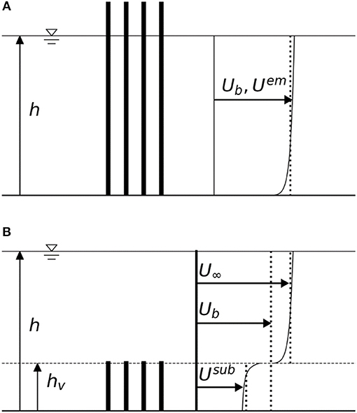
Figure 1. Open channel flows with (A) an emergent canopy and (B) a submerged canopy. In emergent canopies, the depth-averaged velocity ( $\bar{U}$ ) is often used as the representative in-canopy velocity scale (U^em). In submerged canopies, the depth-averaged velocity inside the canopy (U^sub) is often substantially reduced from the above-canopy (free stream) velocity (U_∞).

Emergent Canopies

For emergent canopies, Etminan et al. (2017) proposed to use the theory of drag for isolated cylinders (i.e., Equation 2) as the basis to compute the drag coefficients associated with emergent canopy. Their model employs the constricted cross-section velocity ( $U_{c}^{e m}$ ) as the reference velocity (U_ref) to determine the drag coefficient through the Reynolds number (Equation 2) and to compute the drag force (Equation 3), and was validated through Large Eddy Simulation (Etminan et al., 2017).

Submerged Canopies

For a given in-canopy flow, one can hypothesize that an analogous method to emergent canopies can be applied to submerged canopies, i.e., the in-canopy constricted cross-section velocity ( $U_{c}^{s u b}$ ) can be computed using Equation (4) or (5). However, as discussed in section Introduction, the estimation of $U_{p}^{s u b}$ is not straight-forward due to the vertical variation in the mean velocity profile (Figure 1); the magnitude of the in-canopy velocity both governs, and depends on, the canopy drag. Here, we propose to use a canopy flow model to predict the in-canopy pore velocity ( $U_{p}^{s u b}$ ) based on the (undisturbed) above-canopy flow velocity (U_∞). This model takes the form:

\begin{array}{rcl} U_{p}^{s u b} = U_{\infty} \sqrt{L_{d} / L_{s}} & (7) \end{array}

(Lowe et al., 2005). In Equation (7), L_d is the drag length scale, given by

\begin{array}{rcl} L_{d} = \frac{2 h_{v} (1 - λ_{p})}{C_{d} λ_{f}}, & (8) \end{array}

(Lowe et al., 2005; Ghisalberti, 2009), and represents the flow resistance of the canopy. λ_f is the canopy element frontal area per unit bed area (= h_vd_vN_v). L_s is the shear length scale, given by

\begin{array}{rcl} L_{s} = \frac{2 h_{v}}{C_{f}} & (9) \end{array}

(Lowe et al., 2005) (where C_f is a friction coefficient), which parameterizes the magnitude of the shear stress at the top of the canopy. This shear stress is generated by the velocity difference between the flow within and above the canopy. If velocity measurements are available, the friction coefficient can be estimated based on the peak in the Reynolds stress profile near the top of the canopy (z ≈ h_v):

\begin{array}{rcl} C_{f} = 2 \frac{u_{^{*}}^{2}}{U_{\infty}^{2}} = 2 \frac{{- \bar{u^{'} w^{'}}}_{z \approx h_{v}}}{U_{\infty}^{2}} & (10) \end{array}

(Lowe et al., 2005), where $u_{^{*}}$ is the friction velocity and u′ and w′ are the horizontal and vertical turbulent velocity fluctuations, respectively. Data from a wide range of canopies indicates that $\frac{u_{^{*}}}{U_{\infty}}$ tends to be consistently O(0.1), which corresponds to C_f = O(0.01) (e.g., Harman and Finnigan, 2007; Lowe et al., 2008; Luhar et al., 2010; Moltchanov et al., 2011; Weitzman et al., 2015). Therefore, for a given canopy geometry and above-canopy flow velocity (U_∞), the in-canopy pore velocity $U_{p}^{s u b}$ can be estimated from Equations (7–10). Subsequently, the constricted cross-section velocity inside a submerged canopy can be obtained through Equations (4) or (5), and is used as the reference velocity (U_ref) to calculate the drag coefficient through the Reynolds number (Equation 2) and to compute the drag force (Equation 3).

In summary, the model that is proposed here relies on information on above-canopy flow velocity (U_∞) or bulk velocity (for emergent canopies), the local water depth (h), and the canopy properties: height (h_v), stem diameter (d_v), and canopy density (λ_p, N_v). It includes one empirical parameter (namely, C_f) in the case of a submerged canopy. It is important to emphasize that given the drag coefficient C_d is also needed in Equation (8) to predict the in-canopy flow (hence the drag forces and in-canopy flow are inherently coupled), for submerged canopies the model involves an iterative process. A flow diagram summarizing the model is provided in Figure 2. In the following sections, the model is validated using newly obtained velocity and drag force data, as well as a large dataset covering a broad range in canopy geometries and flow conditions obtained from literature.

FIGURE 2

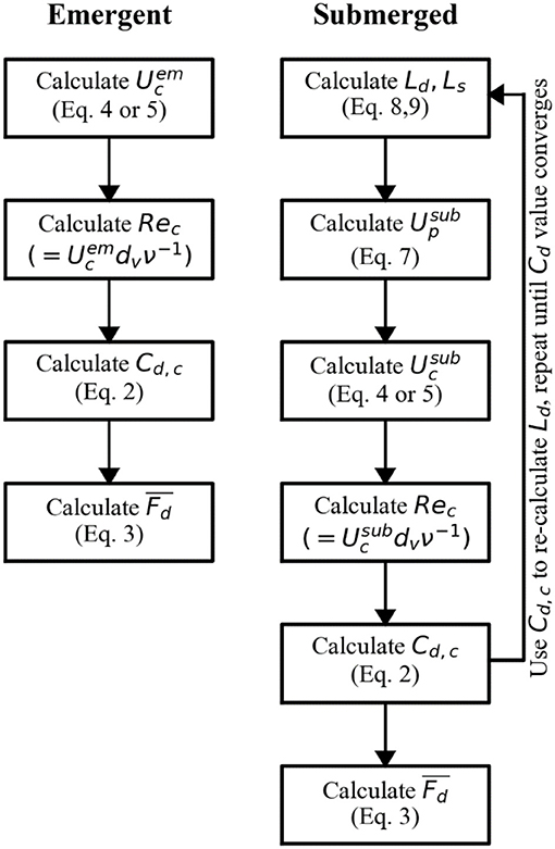
Figure 2. Flow diagram for the canopy drag model. The model can be used to estimate the drag force on an individual element within an emergent or submerged canopy or the bulk canopy drag. As input, it requires above-canopy velocity (U_∞) that can be estimated from the flow rate (Q) or bulk velocity (U_b) for submerged and emergent canopies resp., local water depth (h), and the canopy properties: height (h_v), stem diameter (d_v), and canopy density (λ_p, N_v). For submerged canopies, an initial value of C_d = 1 (to calculate L_d) is suggested.

Experimental Methods

Experiments were carried out in a 20-m-long, 0.6-m-wide, and 0.6-m-deep recirculating flume using emergent (Table 1) and submerged (Table 2) model vegetation. To accommodate the drag force sensor, a 10-cm-high false bottom was placed over a length of 10 m. Model canopies were constructed using perforated PVC sheets and two sets of 6.4-mm-diameter dowels with heights of 30 cm (emergent) or 9 cm (submerged). Dowels were distributed in a staggered arrangement over the entire width of the flume. The dowel diameter used in this study has been used previously in numerous studies to represent a generic aquatic vegetation canopy (e.g., Nepf, 1999) and was originally based on actual observed stem diameters of cordgrass (Spartina alterniflora, see Zavistoski, 1994). An important design parameter for experimental studies with canopies is the canopy length (L_v). Lowe et al. (2005) found a canopy flow adjustment length (x₀) of 3–5 times the drag length scale (L_d) in their experiments. Hence, to ensure fully-developed canopy flow, it was required that L_v >> x₀ resulting in L_v ranging between 2.4 m (λ_p = 0.1) and 3.6 m (λ_p = 0.025).

TABLE 1

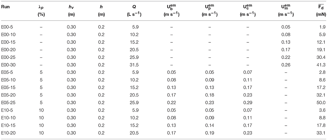
Table 1. Experimental emergent vegetation conditions: canopy density (λ_p), canopy height (h_v), water depth (h), flow rate (Q), bulk velocity ( $U_{b}^{e m}$ ), pore velocity ( $U_{p}^{e m}$ ), constricted cross-section velocity ( $U_{c}^{e m}$ ), measured velocity averaged over the dowel height ( $U_{m}^{e m}$ ) and the measured time-averaged drag force acting on a single cylinder ( $\bar{F_{d}}$ ).

TABLE 2

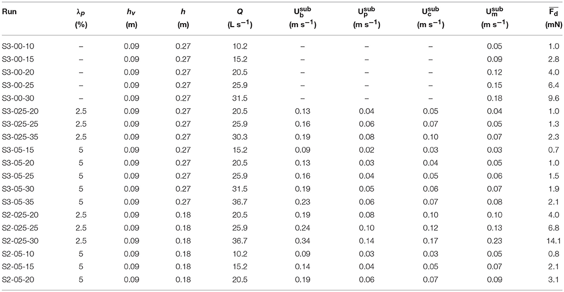
Table 2. Experimental submerged vegetation conditions: canopy density (λ_p), canopy height (h_v), water depth (h), flow rate (Q), bulk velocity ( $U_{b}^{s u b}$ ), pore velocity ( $U_{p}^{s u b}$ ), constricted cross-section velocity ( $U_{c}^{s u b}$ ), measured in-canopy velocity averaged over the canopy/dowel height ( $U_{m}^{s u b}$ ) and the measured time-averaged drag force acting on a single cylinder ( $\bar{F_{d}}$ ).

The drag force exerted on a representative aluminum dowel (canopy element) was measured using a load cell with 2 N capacity (Uxcell, Hong Kong) connected to a load cell amplifier (RW-ST01A, SMOWO, China). The load cell was mounted vertically onto the underside of the false bottom in the flume, ensuring the bottom end of the load cell was fixed but allowing the upper end to move slightly with the bending moment (M_Y) generated by the drag force acting on the dowel (Figure 3). Data was obtained from the load cell using a National Instruments data acquisition system (NI-DAQ PCI-6009) and LabVIEW software. This experimental setup relies on the linear relationship between drag force and the instrument voltage output. To confirm the load cell's linearity, the load cell was placed at the edge of a table and the voltage output recorded for cases with both no weight and a weight of (approximately) 1.9 N. The (linear) calibration coefficient was derived by calculating the ratio between the change in voltage output and the change in applied weight. The linear response was subsequently verified using 9 (smaller) weights ranging from 0.01 to 1.2 N (R² > 0.99). Prior to each individual experimental run, the load cell was re-calibrated using a set of three known weights ranging between 0 and ~0.3 N.

FIGURE 3

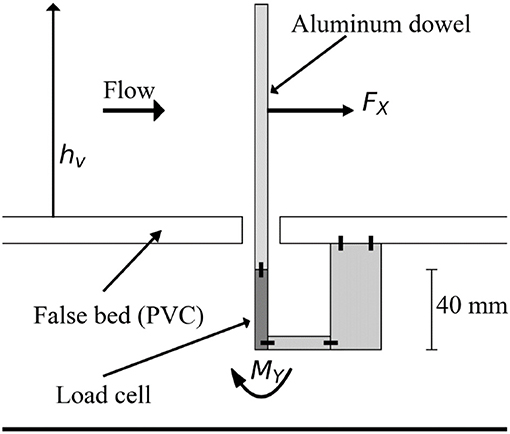
Figure 3. Schematic view of the load cell, which was attached to a single aluminum dowel and placed under the false bed. The drag force (F_x) due to the flow acting on the dowel translates into a moment (M_y) around the base of the load cell.

For emergent canopies, the water level was measured using a point gauge at three locations both upstream and downstream of the canopy. The water level gradient (dη/dx) was then obtained by averaging the water level in time at the upstream and downstream locations and dividing by the canopy length. To calculate the flow rate, velocity measurements were obtained several meters upstream of the canopy using a Nortek Vectrino II Acoustic Doppler Velocity (ADV) profiler, resulting in 3-cm-tall velocity profiles with 1 mm resolution. The vertical position of the ADV was varied to obtain a full velocity profile extending from the bottom to ~5 cm below the water surface. In a similar manner, the velocity profile in and above the canopy was obtained for the submerged cases, and extended from the base of the canopy up to ~5 cm below the water surface. The ADV was positioned within the constricted cross-section in between two canopy elements at a lateral distance of ~0.25S_{v, l} from one of the elements. This was based on the modeling of Etminan et al. (2017), who found that the velocity at this point in a staggered canopy was similar to the constricted cross-section value. Experimental runs were repeated several times to obtain the full velocity profile over depth within and above the canopy. Both the load cell and ADV were placed at a distance of ~2/3 of the canopy length downstream from the leading edge, which is at least 10 times the drag length scale (L_d) for all cases.

The experimental program included a range of canopy densities (λ_p = 0.025, 0.05, and 0.10), canopy submergence ratios (h/h_v = 1, 2, and 3, where h is the water depth at still water and h_v is the canopy height) and flow rates (Tables 1, 2). The upstream flow velocity ranged between ~0.05 and 0.35 m/s, which in combination with the range in canopy density and submergence ratio covers a broad range of conditions that can be found in aquatic canopies. The drag force and velocity data were processed and the drag coefficient was subsequently computed using Equation (3).

Following Taylor (1997), measurement uncertainties were propagated, with an estimated velocity uncertainty of 0.1 cm/s and drag force uncertainty of 0.4 mN. For the model-data comparison the model skill was quantified using scatter index (SCI), and the relative bias. The scatter index is a relative measure of the scatter between computed (x_c) and measured data (x_m) and is computed by normalizing the root-mean-square error ( $\sqrt{\bar{{(x_{c} - x_{m})}^{2}}}$ ) with the maximum of the root-mean-square-value of the data ( $\sqrt{\bar{{(x_{m})}^{2}}}$ ) and the absolute value of the mean of the data ( $| \bar{x_{m}} |$ ). The relative bias is a relative measure of the bias or mean error ( $\bar{(x_{c} - x_{m})}$ ) and is normalized in the same way as the scatter index.

To date only relatively few studies have used load cells to measure canopy drag, hence a comparison is made between the drag force measured directly using the current methodology (F_{d, direct}) and the drag force obtained through an indirect measuring method commonly used in previous studies [F_{d, momentum}, from Equation (6)]. The indirect estimate (F_{d, momentum}) for the emergent cases (E05 and E10, see Table 1) shows the same trend (R² = 0.99) as the drag force directly measured with the load cell (F_{d, direct}, see Figure 4). Although measured drag forces with magnitudes above 0.01 N are very similar for both methods (up to 8% difference), for drag forces < 0.01 N the discrepancy between both methods increases (with an average 22% difference). For these low flow cases the percentage uncertainty associated with the measured water level gradient increases (with the water level dropping only ~3 mm over the length of the canopy) leading to larger errors. Given the high instrument linearity, the force sensor is able to provide more accurate measurements for these cases and is therefore preferred.

FIGURE 4

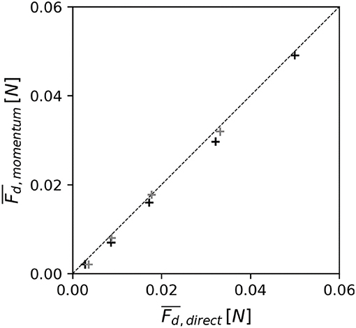
Figure 4. The strong agreement in estimated drag forces on an individual element in an emergent canopy using two methods: (i) measured directly using the force sensor (F_{d, direct}) and (ii) derived indirectly from the water surface gradient (F_{d, momentum}). Marker color indicates canopy density (black: λ_p = 0.05; gray: λ_p = 0.10). The size of the markers indicates the associated measurement uncertainty. The dashed line represents the line of perfect agreement.

Results and Discussion

Measurement of Drag Coefficients

Isolated Cylinder

Although the focus in this study is on assessing canopy drag, a limited number of experiments were conducted with isolated emergent (Table 1) and submerged (Table 2) cylinders. The isolated cylinder drag coefficients were then compared to theory (Equation 2) to gain confidence in the experimental methodology (particularly the drag force data obtained from the load cell). For the emergent case, there is excellent agreement between the directly-measured drag on an isolated cylinder and Equation (2) (Figure 5, squares). For the submerged case (with same height as the submerged canopy), the value of C_d derived from the measured drag force and measured in-canopy velocity (averaged over the cylinder height) is consistent with isolated cylinder theory (Figure 5, triangles). In other words, despite the single vertical cylinder occupying a fraction of the water column in a boundary layer flow, its forces can be predicted by Equation (2) originally developed for a cylinder in a uniform cross-flow.

FIGURE 5

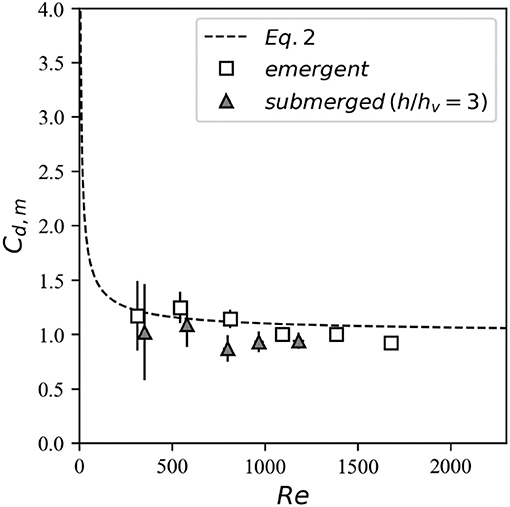
Figure 5. Drag coefficients derived from the velocity and drag force measurements for the isolated cylinder cases.

Emergent Canopies

As discussed in the Introduction, for emergent canopies, both the bulk velocity and pore velocity are often used as the reference velocity in Equation (3) to relate a given flow condition to the canopy drag force through a drag coefficient (i.e., C_{d, b} and C_{d, p}, respectively). Here, when using both the bulk velocity ( $U_{b}^{e m}$ ) and pore velocity ( $U_{p}^{e m}$ ) are used as the drag reference velocity, there are large discrepancies with values for isolated cylinders (Equation 2), similar to results reported in other studies (e.g., Liu and Zeng, 2017). For the highest density canopies (λ_p = 0.1), there is an exponential decrease in the drag coefficient with Reynolds number using both the bulk velocity $U_{b}^{e m}$ (Figure 6A, squares) and pore velocity $U_{p}^{e m}$ (Figure 6B). For the 5% density emergent canopies, the drag coefficient shows a slight decrease with Re using both reference velocities. When considering both $U_{b}^{e m}$ and $U_{p}^{e m}$ , the drag coefficient appears to take an approximately constant value at high Re (i.e., Re >1,000), consistent with other studies (e.g., Tang et al., 2014). Given that the pore velocity accounts for the volume of water being occupied by the canopy, C_{d, p} is always smaller than C_{d, b}, but still deviates substantially from isolated cylinder values. To account for these discrepancies, previous studies have arrived at highly empirical C_{d, p}-Re_p relationships that are parameterized as a function of canopy density (Tanino and Nepf, 2008) and (sometimes) stem diameter (Sonnenwald et al., 2018).

FIGURE 6

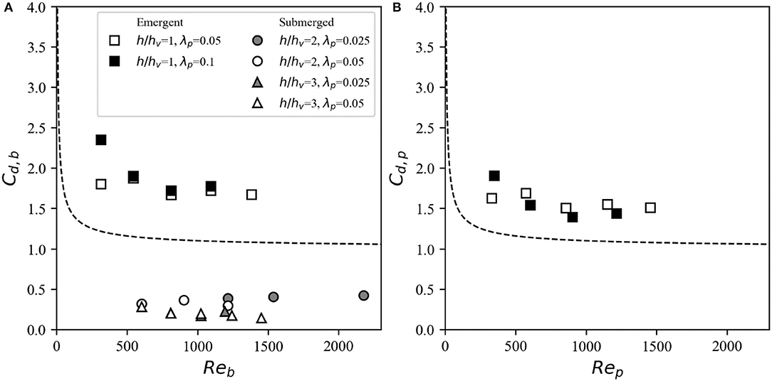
Figure 6. Drag coefficients derived from the drag force measurements using (A) the bulk velocities $U_{b}^{e m}$ and $U_{b}^{s u b}$ and (B) the pore velocity $U_{p}^{e m}$ as the reference velocity for the emergent (squares) and submerged (circles: h/h_v = 2; triangles: h/h_v = 3) cases. The marker color represents the canopy density (black: λ_p = 0.1; white: λ_p = 0.05; gray: λ_p = 0.025), with theoretical values for an isolated cylinder (Equation 2) denoted by the dashed line.

The direct experimental measurements support the canopy drag model proposed by Etminan et al. (2017)–when the constricted cross-section velocity ( $U_{c}^{e m}$ ) is used as the reference velocity, calculated drag coefficients closely match the isolated cylinder values (Figure 7, squares). Therefore, while the drag coefficients derived using the bulk and pore velocities exhibit significant scatter (Figure 6), the use of $U_{c}^{e m}$ in the drag coefficient (C_{d, c}) calculations serves to collapse the data onto the isolated cylinder curve. For the range of Reynolds numbers investigated (Re_c = 380–1,680), the drag coefficients for the emergent cases show relatively little scatter and approaches a canonical isolated cylinder value of C_{d, c} ≈ 1.

FIGURE 7

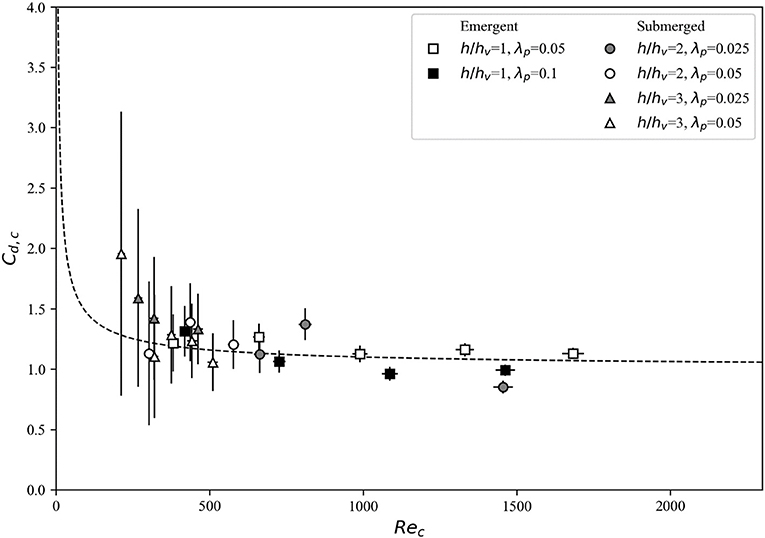
Figure 7. Drag coefficients derived from the drag force measurements for all canopies using the constricted cross-section velocity U_c as the reference velocity for the emergent and submerged cases. Theoretical values for the drag coefficient of an isolated cylinder (Equation 2) are denoted by the dashed line.

Submerged Canopies

The velocity exhibits more vertical variation in submerged canopies than in emergent canopies due the drag discontinuity and resulting shear layer present at the top of the canopy. When using the bulk velocity $U_{b}^{s u b}$ as the reference velocity to derive Re_b and C_{d, b}, relatively low drag coefficients (that substantially deviate from the isolated cylinder values) are obtained (Figure 6A, circles and triangles). This approach neglects the effect of canopy drag on reducing the in-canopy velocity, which is significant at higher canopy densities. Hence, we use measured $U_{c}^{s u b}$ obtained approximately within the constricted cross-section area and derive the associated drag coefficients. For the submerged canopy cases, the measured values of C_{d, c} (i.e., evaluated using the constricted cross-section velocity $U_{c}^{s u b}$ ) generally follows the isolated cylinder theory curve (Figure 7). There is more scatter at Re_c < 500, which can be attributed to the greater uncertainty associated with measuring flow and forces at such low Reynolds numbers. Therefore, analogous to the emergent canopy observations in Figure 6, where C_d evaluated using bulk and pore velocities deviates markedly from isolated cylinder theory, these results indicate that the constricted cross-section velocity $U_{c}^{s u b}$ is the optimal reference velocity for evaluation of drag of a submerged canopy (Figure 7).

Canopy Drag Model Assessment

Emergent Canopies

The canopy drag model for emergent canopies, based on Equations (2)–(4) using the computed constricted cross-section velocity $U_{c}^{e m}$ (see section Canopy Drag Model), was used to predict the drag force on a single canopy element in all experimental cases (Table 1). These predictions were then compared to the time-averaged drag force measured by the force sensor (Figure 8, squares). Using only the bulk flow velocity, which was derived from the known flow rate, and canopy geometry as model input, the canopy drag forces are accurately predicted over the full range of experimental cases. The results provide direct experimental validation of the finding of Etminan et al. (2017) that the constricted cross-section velocity $U_{c}^{e m}$ is the most appropriate reference velocity to parameterize canopy drag.

FIGURE 8

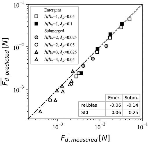
Figure 8. The strong agreement between predicted and measured drag forces, including the line of perfect agreement (dashed). The predictive model skill is described by the relative bias and scatter index (bottom right corner).

Submerged Canopies

To assess the ability of the model to predict the drag of submerged canopies, we first compared the predicted in-canopy velocities with the experimental measurements. Specifically, we compared the measured time-averaged constricted cross-section velocity integrated over the canopy height ( $U_{m}^{s u b}$ ) with predicted $U_{c}^{s u b}$ values, which generally reveals good agreement (Figure 9). The model (with above-canopy velocity and canopy geometry as input) is subsequently applied to calculate the drag force for all submerged canopy cases (Table 2). Canopy friction coefficient values were derived for each case through Reynolds stress profiles (Equation 10), resulting in a range of C_f values between 0.01 and 0.04. However, due to the experimental setup in this study, that used a downward facing ADV, the velocity measurement was limited to measuring only ~6 cm below the water surface. The above-canopy velocity is therefore likely underestimated, particularly in the h/h_v = 2 cases, and actual C_f values are expected to be lower. Due to this uncertainty, here we opt to use a conventional value of 0.01 for all experimental cases (see section Canopy Drag Model). Compared to emergent canopies, there is greater scatter in the relationship between measured and predicted forces (particularly at low Re), but overall there is still relatively good agreement (Figure 8). Given the complexity involved with submerged canopies (including the uncertainty involved with measurements under low Re), and the range in submergence ratio and density investigated, the model error averages about 11% (SCI = 0.114), and suggests that the whole model outlined in Figure 2 can serve as a useful tool to obtain robust estimates of canopy drag forces.

FIGURE 9

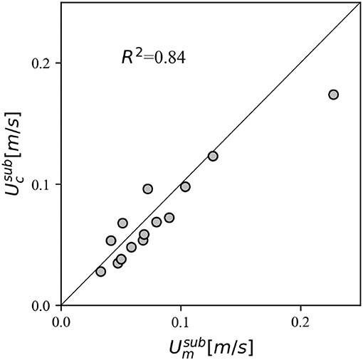
Figure 9. Comparison between the measured depth-averaged in-canopy flow velocity ( $U_{m}^{s u b}$ ) and the estimated in-canopy constricted cross-section velocity ( $U_{c}^{s u b}$ ) in submerged canopies.

Model Application to Other Submerged Canopy Data Sets

To date, the canopy drag model has been validated for emergent canopies (Etminan et al., 2017) (albeit using only numerical simulations); here we have provided direct experimental validation for both emergent and submerged canopies for the first time. Nevertheless, the experiments only covered a relatively small range of possible canopy geometry and flow conditions. To further assess the validity of the model across a large range of flow conditions and canopy properties (e.g., density, submergence ratio, flexibility), the model was tested against a large number of existing datasets. Experiments were limited to those with submerged canopies in which the energy slope was reported.

Rigid Vegetation

For rigid vegetation, experiments that employed either staggered (as in the present study), linear or random arrangements were selected here (Table 3). Although on the individual canopy element scale, the velocity distribution may vary significantly among these arrangements, we hypothesize that the model can still be used to estimate bulk canopy drag. Indeed, the work of Etminan et al. (2017) suggested that in the case of randomly-distributed canopy elements, the constricted cross-section velocity can still be considered as the velocity scale governing canopy drag, indicating that the model can be applied here without modification. Hence, using provided values of flow rate and canopy properties, the bulk drag was computed and compared with the measured drag (Figure 10A). Using a constant C_f value of 0.01 (as before), the model shows a similar trend as the measurements (R² = 0.74) with reasonably low bias and scatter (rel. bias = 0.02, SCI = 0.45). It should be emphasized that the main uncertainty is likely to be attributed to the schematization of relatively complex three-dimensional canopy hydrodynamics into a relatively simple (two-layer) model.

TABLE 3

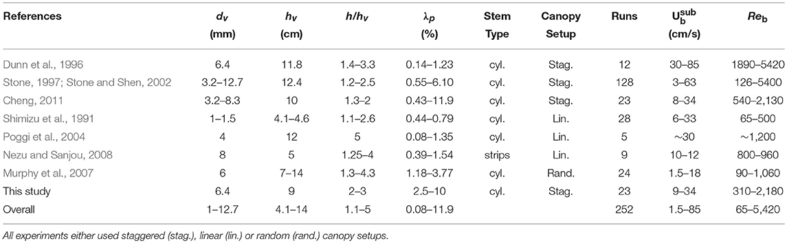
Table 3. Overview of experimental studies on drag in submerged rigid canopies from which data was obtained.

FIGURE 10

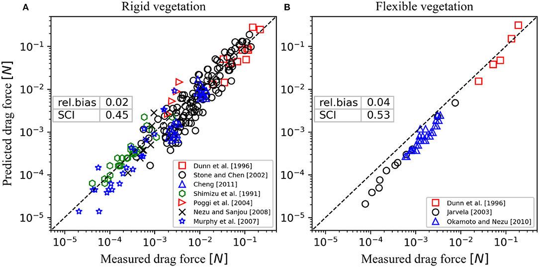
Figure 10. Validation of canopy drag model for submerged canopies against previous experimental results with (A) rigid and (B) flexible vegetation (listed in Tables 3, 4, respectively).

Flexible Elements

Although most studies so far have represented vegetation canopies using rigid elements, aquatic vegetation in natural systems is often flexible (e.g., seagrasses, kelp), adapting its shape and thereby frontal area in response to the flow. Hence, there is now increased experimentation with flexible mimics in hydraulic experiments (e.g., Abdolahpour et al., 2017). The canopy drag model presented in this study does not explicitly account for flexibility, but it is hypothesized that it could still be used as a tool provided the deflected vegetation height (i.e., the height of the vegetation under stationary flow condition) rather than the actual length of the element is used. Hence, data was obtained from three studies that investigated drag in submerged flexible canopies and reported the deflected canopy height (Table 4). From these studies, both Dunn et al. (1996) and Järvelä (2003) observed swaying motions of their flexible plants/(cylindrical) elements, resulting in a time-varying deflected canopy height. Okamoto and Nezu (2010) reported both swaying and the more organized monami-type motions (Ackerman and Okubo, 1993) in their experiments. Here, we use the time-averaged deflected canopy height as input for the model. Furthermore, for the experiments by Okamoto and Nezu (2010) we use the width of the flexible strip as a proxy for d_v given that it is equivalent to the frontal area.

TABLE 4

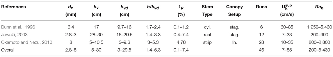
Table 4. Overview of experimental studies on drag in submerged flexible canopies from which data was obtained.

For the flexible canopies, the model is able to predict the bulk drag relatively well (Figure 10B, R² = 0.69, rel. bias = 0.04, SCI = 0.53). This is surprising to some extent, as the complexity associated with flexible elements is only accounted for to some extent by the (deflected) plant height. Both the measurements by Järvelä (2003) and Okamoto and Nezu (2010) are consistently underpredicted, which may be related to the plant geometries that involved flat strips and real plants, respectively. Dunn et al. (1996), on the other hand, used flexible cylinders in their experiments which provide more similarity with rigid cylinders, and may therefore better be represented by model.

Overall, with limited information (above-canopy velocity derived from flow rate, canopy properties) the relatively simple canopy drag model is able to provide reasonably accurate estimates of the bulk canopy drag for both rigid and flexible vegetation canopies. Given the fact that the model performs well over such a broad range of hydrodynamic conditions (U_b = 1.5–85 cm/s, Re = 65–5,430) and canopies (h/h_v = 1.1–5, λ_p = 0.08–11.9%, both rigid and flexible vegetation), and is based on theory rather than empirical relations, it is thus expected the model can robustly predict hydraulic resistance of aquatic canopies, including in field setting with natural vegetation (e.g., where stem diameters are often of order 0.1–1 cm and current velocities of order 0.05–0.5 m/s, which translates to Re ranging between 50 and 5,000).

Summary and Conclusions

In this study we present new direct experimental measurements of canopy drag forces using emergent and submerged canopies with a broad range of flow conditions and canopy properties (i.e., density and submergence ratio). Drag coefficients were derived using direct measurements of the drag force on a dowel within the canopy. We found that if the constricted cross-section velocity is used as the reference velocity, the drag coefficient of both emergent and submerged canopies is equal to that of an isolated cylinder. Comparison between canopy drag model predictions and current and existing experimental data shows that the model is able to robustly and accurately predict canopy drag across the field range of flow conditions and canopy characteristics, including flexible canopies. The model can thus be used to predict drag forces in emergent and submerged canopies and is considered a simple and practical tool for estimating the hydraulic resistance of aquatic canopies.

Data Availability Statement

The datasets analyzed for this study can be obtained by sending a written request to the corresponding author at arnold.vanrooijen@research.uwa.edu.au.

Author Contributions

AvR designed the experiments, acquired the data, performed the data analysis, and wrote the manuscript. RL and MG provided support in the experimental design, data interpretation and the development of the manuscript. MC-F and LT provided support in data acquisition during the experiments. All authors revised the draft manuscript and approved the final version for submission.

Funding

This work was supported by an Australian Research Discovery Project Grant (DP170100802) to RL and MG.

Conflict of Interest Statement

The authors declare that the research was conducted in the absence of any commercial or financial relationships that could be construed as a potential conflict of interest.

Acknowledgments

This research was undertaken by AvR as part of a Ph.D. at The University of Western Australia who was funded by a University Postgraduate Award for International Students (UPAIS) and an Australian Government Research Training Program (RTP) Scholarship. LT was supported by the China Scholarship Council (grant number: 201706320274). The authors would like to thank Mr. Carlin Bowyer, Ms. Dianne King, and Mr. Brad Rose for assistance in the lab, Dr. Guido Wager for providing support with the force sensor, Dr. Vahid Etminan for valuable discussions, and the reviewers for their constructive feedback that helped to improve the manuscript.

References

Abdolahpour, M., Hambleton, M., and Ghisalberti, M. (2017). The wave-driven current in coastal canopies. J. Geophys. Res. Oceans 122, 3660–3674. doi: 10.1002/2016JC012446

ORIGINAL RESEARCH article

Predicting Current-Induced Drag in Emergent and Submerged Aquatic Vegetation Canopies

Introduction

Canopy Drag Model

Emergent Canopies

Submerged Canopies

Experimental Methods

Results and Discussion

Measurement of Drag Coefficients

Isolated Cylinder

Emergent Canopies

Submerged Canopies

Canopy Drag Model Assessment

Emergent Canopies

Submerged Canopies

Model Application to Other Submerged Canopy Data Sets

Rigid Vegetation

Flexible Elements

Summary and Conclusions

Data Availability Statement

Author Contributions

Funding

Conflict of Interest Statement

Acknowledgments

References

Notation

This article is part of the Research Topic

People also looked at