Observing Sea States
 Fabrice Ardhuin1*
  Justin E. Stopa2
  Bertrand Chapron1 Fabrice Collard3
  Romain Husson4
  Robert E. Jensen5
  Johnny Johannessen6 Alexis Mouche1
  Marcello Passaro7
  Graham D. Quartly8
  Val Swail9
  Ian Young10
- 1Laboratoire d'Océanographie Physique et Spatiale (LOPS), CNRS, IRD, Ifremer, IUEM, Univ. Brest, Brest, France
- 2Ocean Resources and Engineering, University of Hawaii at Manoa, Honolulu, HI, United States
- 3OceanDataLab, Locmaria Plouzane, France
- 4CLS, Division Radar, Plouzané, France
- 5United States Army Crops of Engineers, Vicksburg, MS, United States
- 6Nansen Environmental and Remote Sensing Center, Bergen, Norway
- 7Deutsches Geodätisches Forschungsinstitut der Technischen Universität München, Munich, Germany
- 8Plymouth Marine Laboratory, Plymouth, United Kingdom
- 9Environment and Climate Change Canada, Toronto, ON, Canada
- 10University of Melbourne, Melbourne, VIC, Australia
Sea state information is needed for many applications, ranging from safety at sea and on the coast, for which real time data are essential, to planning and design needs for infrastructure that require long time series. The definition of the wave climate and its possible evolution requires high resolution data, and knowledge on possible drift in the observing system. Sea state is also an important climate variable that enters in air-sea fluxes parameterizations. Finally, sea state patterns can reveal the intensity of storms and associated climate patterns at large scales, and the intensity of currents at small scales. A synthesis of user requirements leads to requests for spatial resolution at kilometer scales, and estimations of trends of a few centimeters per decade. Such requirements cannot be met by observations alone in the foreseeable future, and numerical wave models can be combined with in situ and remote sensing data to achieve the required resolution. As today's models are far from perfect, observations are critical in providing forcing data, namely winds, currents and ice, and validation data, in particular for frequency and direction information, and extreme wave heights. In situ and satellite observations are particularly critical for the correction and calibration of significant wave heights to ensure the stability of model time series. A number of developments are underway for extending the capabilities of satellites and in situ observing systems. These include the generalization of directional measurements, an easier exchange of moored buoy data, the measurement of waves on drifting buoys, the evolution of satellite altimeter technology, and the measurement of directional wave spectra from satellite radar instruments. For each of these observing systems, the stability of the data is a very important issue. The combination of the different data sources, including numerical models, can help better fulfill the needs of users.
1. Introduction
The development of modern measurements and prediction of sea states has been strongly linked to naval and shipping activities. Here we will define “sea state” rather narrowly as surface gravity waves with periods shorter than 5 min, but this “sea state” is obviously studied in a wider context of all the sea conditions that affect navigation, including winds, currents, and sea ice. We cannot ignore winds and currents that, together with sea ice, are the forcing agents that define the properties of waves, with some possible feedback of waves on these other phenomena. This is discussed by Villas Bôas et al. (2019). Here we only focus on surface gravity waves, which are of interest for a very broad range of applications.
Sea states have been observed for a few centuries, either as the main reason for the measurement, as in ship logs (Gulev et al., 2003), or as a by-product of other observations. Indeed, ocean waves have an obvious signature in many other measurements ranging from seismic observations (Bertelli, 1872) to ocean remote sensing, such as sea level monitoring from satellite altimeters (Minster et al., 1991), or radiometric measurements of winds and salinity (e.g., Reul and Chapron, 2003).
All of these measurements, either made on purpose or arising from other applications, have important uses for human activities at sea and on the coast. In particular, waves affect shipping and harbor operations, with data provided by meteorological services under the Safety of Life at Sea (SOLAS) convention, which is why many wave buoys around the world are managed by port authorities or located near important harbors, while naval architecture still relies primarily on visual observations (Bitner-Gregersen et al., 1995; IACS, 2001). Other applications have developed very localized measurement systems, in particular for coastal hazards and beach morphodynamics (e.g., Holman and Stanley, 2007). Except for the recent launch of CFOSAT (Hauser et al., 2017), measuring ocean waves has not been the primary goal for satellite missions. Still, these data are very useful but the observing system has not been optimized to sample storms in space and time. Wave observations are particularly useful for the investigation of air-sea fluxes of momentum and heat (Cronin et al., 2019), gas, aerosols (Veron, 2015) and parameterizations in weather predictions or climate models. Similarly, the ever-growing network of seismic stations on land (Romanowicz et al., 1984; Tytell et al., 2016) are providing opportunities for long-term sea state monitoring, even in remote locations (e.g., Bromirski et al., 1999; Ardhuin et al., 2012; Retailleau et al., 2017), or, at the very least, some independent data for validating trends of other observing systems.
All existing observations, as well as emerging new technologies, are complementary. Starting from the analysis of requirements from user communities in section 2, we review today's wave observations in section 3, and, in section 4, look forward to the next decade on how these could be better organized and exploited to map the space and time variability of sea states. Recommendations follow in section 5.
2. Requirements for Sea State Measurements and Connection With Other Essential Climate Variables
Although this paper is focused on wind-generated waves, the importance of the forcing factors that are the wind, currents and sea ice cannot be ignored, and they are very important when interpreting observations or validating numerical models.
2.1. General Definitions
Here we consider that statistical properties of the surface elevation are fully described by the wavenumber-direction wave spectrum F(k, θ), which describes how the surface elevation variance is distributed across wavenumbers k and directions θ, with θ the direction from1 which the waves are propagating, hence opposite to the direction of the wavenumber vector k. Possible correction for non-linear effects are given by Fedele and Tayfun (2007) and Janssen (2009), with one particular application demonstrated by Leckler et al. (2015). This approach is most appropriate for waves in deep water. It is customary to transform wavenumbers to frequencies using the linear dispersion relation
where g is acceleration due to gravity, D is the water depth, and σ is the relative radian frequency. Currents are accounted for using
where ω = 2πf is the absolute radian frequency, as measured in a frame of reference attached with the solid Earth, and UA is the phase advection velocity that is generally a function of the wavenumber vector k (Stewart and Joy, 1974; Andrews and McIntyre, 1978). The radian frequency σ = 2πfr is the relative frequency that would be measured in a reference frame moving with the velocity UA.
This dispersion relation gives a frequency-direction wave spectrum, with an example shown in Figure 1
The difference between f and fr is particularly important in the presence of currents faster than 0.2 m/s. For completeness, we briefly recall the definitions of common sea state parameters (IAHR Working Group on Wave Generation and Analysis, 1989).
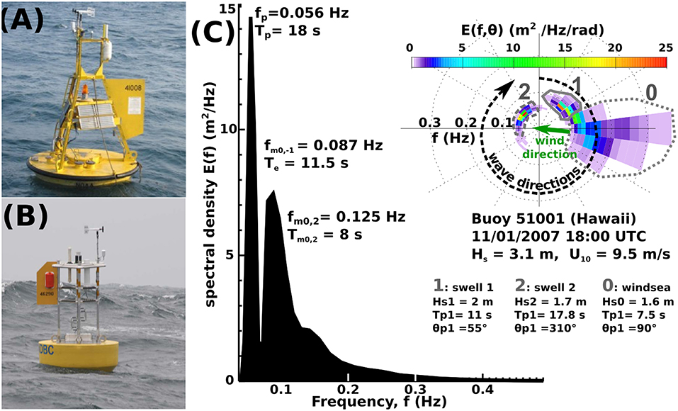
Figure 1. (A,B) show typical layout of NBDC wave buoys with old and new designs. Wave measurements are made by a motion package in the hull and wind measurements use an anemometer at 5-m height. (C) Example of wave information derived from a buoy, ranging form the common estimate of Hs to the heave spectrum E(f) in black, or a two-dimensional directional spectrum E(f, θ) in colors. Note that the buoy does not measure the directional spectrum but, for each frequency, only the “First 5” parameters from which the directional spectrum is estimated here using the Maximum Entropy Method (Lygre and Krogstad, 1986). For many applications it is customary to partition the spectrum into a windsea region (dotted contour labeled 0), and swells (solid and dashed contours labeled 1 and 2) which are usually ordered by decreasing wave energy. For each partition, height, period and direction parameters are estimated in the same manner as they would be estimated from a full (frequency-direction) spectrum.
The significant wave height Hs is defined as 4 times the standard deviation of the surface elevation,
with other usual notations SWH and Hm0. The surface heave spectrum is
For each frequency, another four parameters are readily measured from the spectra and co-spectra of three co-located time series of wave-associated variables such as the heave, pitch and roll of a surface-following buoy (Cartwright and Longuet-Higgins, 1956), or its 3-component acceleration vector, or the combination of pressure and horizontal velocity. These are
The combination of E(f), a1(f), b1(f), a2(f), b2(f), or any other equivalent parameters (Kuik et al., 1988), forms the set of “First 5” spectral wave parameters.
One year of hourly wave directional wave measurements contains roughly 8,760 records, and a “First-5” dataset with 50 frequencies would have 250 data points for each record. These 2.2 × 10⁶ data values per year provide a much better description of the sea state than a much reduced set of a few integrated parameters that is necessary for many applications.
For the purpose of providing weather information or for comparing different sensors, it is useful to use a reduced set of values. For this spectral partitioning methods are very useful in associating energy to a common peak, which is a great way to analyze swell data (Gerling, 1992; Hanson and Phillips, 2001; Portilla et al., 2009). This is illustrated with the gray contours on Figure 1C.
Mean wave periods are generally estimated from moments of the wave spectrum as follows for the pth moment period,
These periods, in particular Tm0,2 defined by Equation (10) with p = 2, are sensitive to the practical choice of the maximum frequency fmax. They are also markedly different in the presence of currents when measured with a drifting instrument or with a moored instrument.
We have emphasized currents in these definitions of sea state parameters because of the evidence of the role currents in wave time series (e.g., Ardhuin et al., 2012; Gemmrich and Garrett, 2012). Recent research has further revealed that away from the coast (Magne et al., 2007), even outside the well known boundary currents, ocean currents are the main source of wave height variability at scales under 200 km, as illustrated in Figure 2 (see also Gallet and Young, 2014; Ardhuin et al., 2017a; Quilfen et al., 2018).
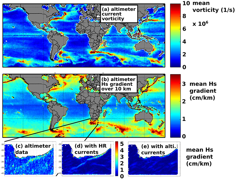
Figure 2. (a,b) show 4-year mean (2013-2016) computed using the constellation of 4 satellite altimeters, of current vorticity estimated from gridded altimeter data, and along-track gradient of significant wave height. (c) is a higher resolution grid over the Agulhas current for August 2015, compared to (d) a WAVEWATCH III model run forced by 1-km resolution modeled currents, and (e) forced by altimeter-derived gridded currents (Adapted from Quilfen et al., 2018 as authorized by Elsevier).
2.2. Updating Requirements for Sea State Measurements
Sea states are thus much less uniform than previously imagined, with important consequences for applications. Also, the importance of waves for coastal sea level (Ponte, 2019), is naturally providing requirements for the accuracy and stability of wave heights and periods that are key variables for explaining extreme sea level (e.g., Stockdon et al., 2006; Poate et al., 2016; Dodet et al., 2018). In particular, consistency with the requirements on mean sea level, is calling for an adjustment on the requirements for sea state as previously defined by GCOS-200 (Belward, 2016). Given that the maximum run-up is of the order of the offshore significant wave height, we may specify separate requirements for the sea state parameters at large (global to regional) scales, and stricter requirements for coastal sea state parameters, which should apply right outside of the surf zone, as proposed in Table 1.
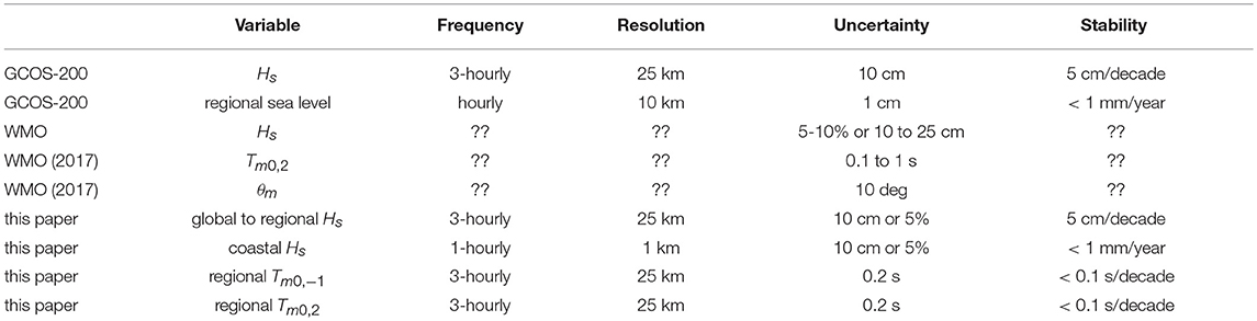
Table 1. Requirements on sea state measurements according to GCOS-200, and propositions for updates. The requirements on stability should be understood as applicable to all percentiles of the heights or period distributions.
Accuracy levels of directional wave measurements required by various user groups vary as already identified at OceanObs'09 (Swail et al., 2009). However if the most stringent requirement is followed then the needs of the diverse user groups and applications will be met. This requires centimeters for wave heights, tenths of seconds for wave periods, and 2–5° for directions.
The WMO (World Meteorological Organization) lists the wave requirements in detail for various applications (WMO, 2017a,b). Typically, these requirements specify significant wave height accuracy of 5–10% (or 10–25 cm); wave periods of 0.1–1 s, wave directions to 10°, and wave spectral densities to 10 percent. For certain applications, especially in coastal regions, required accuracies are higher, which presents significant challenges.
Enforcing these requirements for any directional wave measurement system, a genuine ground-truth would be established.
Quantification of multi-component wave systems with differing directions at the same frequency can affect various wave related applications, this is particulary the case for waves in opposing directions in the case of microseism sources (Hasselmann, 1963; Obrebski et al., 2012). Therefore, the accuracy and resolution of the wave directions are critical.
Buoy technology is available that can provide good quality measurements for the 'First 5' parameters (Equations 5–9). The generalization of such technology and the monitoring of the data quality is further discussed below.
New and future satellites such as CFOSAT (Hauser et al., 2017) and SKIM (Ardhuin et al., 2018) should be able to go beyond these “First 5,” with unprecedented directional resolution, but their temporal sampling cannot make them the backbone of a sea state monitoring system. Still, such new data can provide a transformation of our understanding and advance our numerical modeling capabilities.
This was demonstrated in the last decade with swell monitoring from SARs (Ardhuin et al., 2009) leading to the development of new parameterizations for wave dissipation by Ardhuin et al. (2010) leading to a typical 30% error reduction in Hs estimates (see Figure 3 and Roland and Ardhuin, 2014). These parameterizations are now used at most wave forecasting centers: these include Meteo-France since 2010, NCEP since 2012, the Bureau of Meterology since 2010, and ECMWF in June 2019 with the cycle 46r1 of their Integrated Forecasting System, after demonstration at LOPS since 2008. Unfortunately the ECMWF ERA5 reanalysis uses an older version Cycle 41r2 (Hersbach and Dee, 2016).
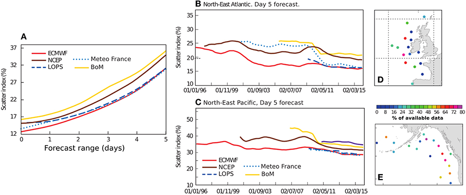
Figure 3. (A) Scatter index for Hs from 5 numerical wave forecasting systems against a selection of mostly Northern Hemisphere wave buoys, as a function of forecast range, for the months of September 2015 to August 2016. These forecasts are produced by ECMWF (Reading, UK, with reanalysis available as ERA5), NOAA/NCEP (MD, USA), Meteo-France (Toulouse, France, now available as part of the Copernicus Marine Environment Monitoring Service, marine.copernicus.eu), the Bureau of Meteorology (Melbourne, Australia) and LOPS (Brest, France, available in hindcast at ftp://ftp.ifremer.fr/ifremer/ww3/HINDCAST/). Focusing on the 5-day forcasts, (B,C) show the evolution of the model error with the years, at selected buoys in the North-East Atlantic and the North-East Pacific, with locations shown in (D,E). Adapted from Bidlot (2016) as authorized by ECMWF.
Satellite data are also used at Meteo-France and ECMWF for correcting the initial conditions of wave models, and in the production of reanalyses. Whatever their use, whether for improving model parameterizations or for assimilation in forecasting and reanalyses, satellite data ultimately relies on the calibration and validation using in situ buoys (e.g., Stopa et al., 2016).
2.3. Trends and Interannual Variability
A specific aspect of observation requirements is the stability of the estimates of sea state parameters. The wide range of estimates of trends in wave heights, from Young et al. (2011) to Hemer et al. (2013) is certainly calling for modesty when defining requirements on the stability of sea state estimates. Understanding past trends is necessary if one wishes to extrapolate them in the future, here are two examples.
In the Southern Ocean, there is growing evidence from both in situ measurements and model studies that westerly winds intensified from 1987 to 2011 (Hande et al., 2012), partly associated with a general expansion of the tropics caused by global warming (Lucas et al., 2014), and partly due to an increase in extension of the sea ice which persisted up to 2014 (Turner and Comiso, 2017).
In the tropical Pacific, the contribution of inter-annual variability patterns is particularly strong, these include the El Nino Southern Oscillation and the longer Interdecadal Pacific Oscillation, IPO (Fyfe et al., 2014). In particular, trade winds over the west Pacific have increased from 1992 to 2011 associated with a particular phase of the IPO (England et al., 2014; Fyfe et al., 2014). Both of these increases have been reflected in altimeter derived trends across the global ocean (Young et al., 2011), and there is no known physical process that could lead to a long-term sustained trend of that 0.5–2% per year. Other evidence suggests inter-annual variability of Hs is relatively small, typically under 8%, as quantified by wave hindcasts over several decades (Stopa et al., 2013).
Young et al. (2011) estimated Hs trends from 1985 to 2008 using the dataset of Zieger et al. (2009) who calibrated each altimeter mission with respect to moored buoys and by cross-calibrating the different satellite platforms. The Hs calibration with buoy observations was based on nearly 8,000 co-locations. The calibration was performed for Hs <8 m; therefore wave heights above 8 m remain largely unconstrained by direct buoy observations. In tropical storms where Hs are large, there are often heavy rains which might introduce errors (Guymer et al., 1995; Young et al., 2017).
The trends for the 99th percentile (P99) of Hs presented in Young et al. (2011) and adapted here in Figure 4 are much larger (1–5 cm year−1) than the GCOS-200 requirements (Table 1). However, the global trend in average wave height is small with possibly only the Southern Ocean showing statistically significant positive trends (Young et al., 2011). There is a reasonable level of confidence in mean trends determined from satellite data; however, accurately determining trends in upper percentiles is more challenging. Although a comprehensive validation of altimeter performance under such extremes conditions is still lacking, the limited comparisons with buoy data and extrapolations to extreme value conditions indicate that reasonable data can be obtained (Young et al., 2017; Takbash et al., 2019). In addition, however, there needs to be a sufficiently large number of satellite passes to form stable values of the upper percentiles. This is a demanding requirement, as altimeters, with their large spatial separation between ground tracks, tend to under-sample small-scale storms, such as tropical cyclones (Takbash et al., 2019). As a result, questions have been raised about whether stable values of these upper percentiles can be measured and whether the increase in the number of satellites in orbit may introduce a spurious positive trend in long term altimeter estimates. As both the length of the altimeter dataset and the number of satellites in orbit increases our ability to answer these question will improve.
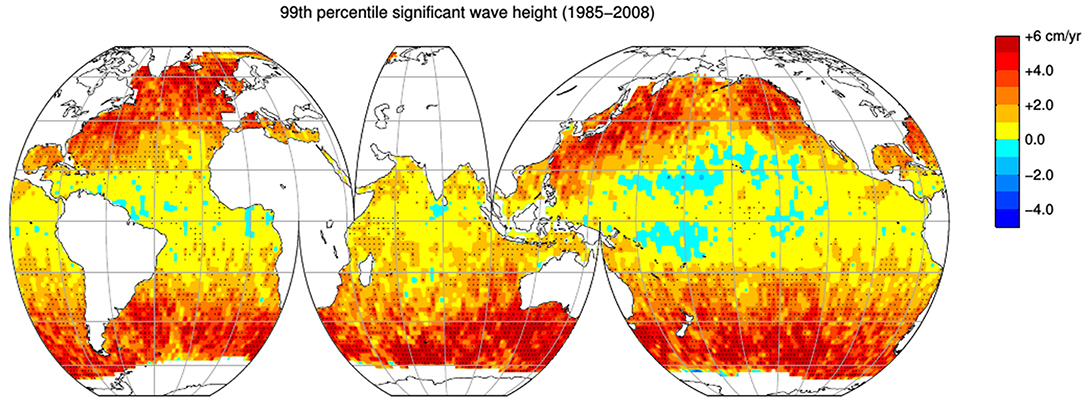
Figure 4. Hs trends computed from a monthly time series of the 99th percentile from the merged altimeter database of Zieger et al. (2009) in 2° bins. The black stippling represents a statistically significant trend at the 99% confidence limit. reprinted from Young et al. (2011), as authorized by AAAS.
Trends for Hs from buoys have been estimated from time series spanning several decades off the West coast of the United States and Canada. These generally show increasing wave heights (Allan and Komar, 2000; Gower, 2002; Menéndez et al., 2008; Ruggiero et al., 2010). However, these trend estimates are strongly distorted by changes in buoy hull, sensor payload, sampling acquisition, and processing (Gemmrich et al., 2011), which we further discuss in section 3.1.
Many wave climate studies conducted using model hindcasts forced by multi-decadal reanalysis datasets (wind fields and ice concentrations) have been conducted (e.g., Wang and Swail, 2001; Caires and Sterl, 2005; Hemer et al., 2009; Fan et al., 2012; Reguero et al., 2012; Stopa et al., 2013). None of these studies correct for the changing quality of the reanalysis wind field that introduces temporal changes as discussed in several studies that use the Climate Forecast System Reanalysis (Chawla et al., 2013; Rascle and Ardhuin, 2013; Stopa and Cheung, 2014). Monthly Hs residuals in Figure 5 with respect to merged satellite radar altimetry dataset reveals spatial as well as temporal changes in the time series. It is clear that the Hs residuals are larger for larger sea states (e.g., Hs P95). The strong change in Hs residuals, namely in the Southern Hemisphere, in 1994 was linked to the inclusion of the SSM/I satellite radiometer into the reanalysis data (Rascle and Ardhuin, 2013). Since the quantity as well as quality of the satellite observations being assimilated into reanalysis datasets changes in time (Saha et al., 2010; Dee et al., 2011), wave hindcasts driven by reanalysis are strongly related to the changes in wind forcing. Therefore, hindcasts in the current status cannot meet the GCOS-200 Hs requirements of 5 cm/decade since Figure 5 shows the Hs residuals are at least 10 cm/decade for the median and 50 cm for the 95th percentile. Certainly, the reference dataset used in this figure, satellite altimeters, also has time and space stability errors.
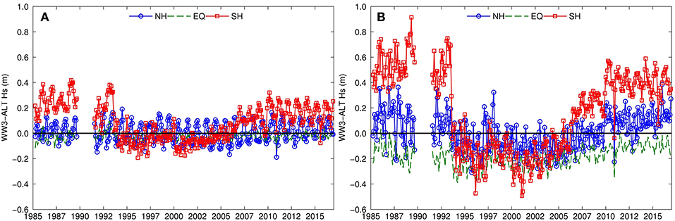
Figure 5. (A,B) show Hs monthly median (50th percentile P50) and P95 residuals: wave hindcast forced by CFSR - altimeter. The statistics are computed for latitudinal bands: Northern Hemisphere (NH: latitude > 30 °N), Equator (EQ: latitude < 30°), and Southern Hemipshere (SH: latitude > 30°S).
The urgency of understanding total sea level at the coast (e.g., Melet et al., 2018) is clearly calling for a stability that matches that of the offshore sea level. This is particularly important in today's transition where the total ice-shelf melt contribution to sea level rise is still limited to a few centimeters. In the long term, with sea level rise of several meters, the few centimeters to decimeters due to waves will probably be less important, except where changes are dramatic, as is the case in the Arctic (e.g., Stopa et al., 2016) and possibly in tropical cyclones (Shimura et al., 2016).
Finally, extreme waves and their trace in the geological record are used as evidence for past storminess using paleo-shorelines (Bouchette et al., 2010), ripple marks (Allen and Hoffman, 2005) or wave-transported boulders (Cox et al., 2016). It is thus very important to link extreme sea states to these geological marks under present climate conditions from shoreline features (Ashton et al., 2001) to ripples (e.g., Ardhuin et al., 2002), and boulders (Autret et al., 2016; Kennedy et al., 2016), in order to better understand the geological record and past climates.
3. Existing Measurement Technologies and Their Limitations
3.1. In-situ Measurements
The majority of existing in-situ wave measurements are made from moored buoys in the coastal margins of North America and Western Europe. There are large data gaps in the rest of the global ocean, particularly in the Southern Ocean and the tropics while other existing observational systems often have considerable coverage in these areas, such as the Argo temperature/salinity profiling floats. Also, sea state measurements are often missing at reference sites where other Essential Climate Variable (ECVs, see WMO, 2004) are measured. This is further discussed in section 4.
For open-water applications, the preferred wave measurement platform is a buoy. Buoys can be spherical, discus, spar, or boat-shaped hull. The most popular and widely used method measures buoy motion and converts the buoy motion into wave motion based on its hydrodynamic characteristics. Once the buoy response is determined for each hull, wave motion can be derived based on the buoy response function.
Directional buoy wave measurements based on buoy motion can be categorized into two types: translational (particle-following) or pitch-roll (slope-following) buoys. For both types, a variety of different sensor technologies is used to measure buoy motion. Since directional wave information is derived from buoy motions, the power transfer functions and phase responses associated with the buoy, mooring, and measurement systems play crucial roles in deriving wave data from buoys (Teng and Bouchard, 2005). This dependence is particularly important at low energy levels and at both short and long wave periods where the wave signal being measured is weak, and potential signal contamination increases.
All of the in-situ wave systems base their directional estimators on the measurements of three concurrent time series, which can be transformed into a description of the sea surface. All devices can provide good integral wave estimates (Hs, peak period, mean direction at the peak period, etc.). However, not all sensors can provide high quality “First-5” estimates because of the inherent inability of the sensor to separate wave signal from electronic and system/buoy response noise. This would degrade the quality of any derived directional wave spectra. In particular, high quality “First-5” observations can be used to resolve two different wave systems at the same frequency, if they are at least 60° apart, whereas other measurement systems cannot. Although there are more than five Fourier coefficients, the “First-5” variables provide the minimum level of accuracy required for a sufficiently accurate directional wave observing system, as it covers both the basic information (Hs, Tp, θm) along with sufficient detail of the component wave systems to be used for the widest range of activities. Going beyond the “First Five” requires an array of sensors (e.g., Krogstad, 2005), or imaging method based on radar or optical data.
As wave measurement systems continue to evolve, with changing hulls, composition, super-structures, moorings, sensors and on-board analysis packages, it is extremely important to maintain readily accessible metadata archives that continually update any change to a platform. Existing moored buoy networks are often legacy systems. Standardization of sensors, system configurations, or hull type would be costly and impractical, and not necessarily desirable. Continuous testing and evaluation of operational and pre-operational measurement systems is an essential component of a global wave observing system, equal in importance to the deployment of new assets. An overriding objective of continuous evaluation is to ensure consistent wave measurements to a level of accuracy that will serve the requirements of the broadest range of wave users. Comparisons of platforms and sensors have been pursued (Schwab and Liu, 1985; Skey et al., 1995; O'Reilly et al., 1996; Teng and Bouchard, 2005; Collins et al., 2014). These efforts are critically important because there were old designs, such as the NOMAD (Timpe and Van de Voorde, 1995) or 3-m discus buoys (Steele et al., 1992) being retired; and it is essential to relate the records of past wave climate, with hundreds of buoy years, to the present and future wave climates.
Another way to monitor the range of buoy hulls, sensors, and processing systems is to use radar altimetry from satellites as reference. This is particularly useful for buoys in open ocean and deep water and locations close to altimeter tracks. Queffeulou (2006) and Durrant et al. (2010) showed mean Hs differences of 10% between the U.S. NOAA-NDBC and the Meteorological Service of Canada (MSC) buoy networks by using the satellite altimeter estimates using as reference. Only part of this difference can be attributed to the fact that the satellite does not measure exactly the same region as the buoy, introducing a small bias and random difference (see also Krogstad et al., 1999).
In October 2008, a wave measurement technology workshop was held (JCOMM, 2008), with broad participation from the scientific community, wave sensor manufacturers and wave data users, following on from a March 2007 Wave Sensor Technologies Workshop (Alliance for Coastal Technologies, 2007). The overwhelming community consensus resulting from those workshops was that:
• The success of a wave measurement network is largely dependent on reliable and effective instrumentation.
• A thorough and comprehensive understanding of the performance of existing technologies under real-world conditions is currently lacking.
• An independent performance testing of wave instruments is required.
The workshops also confirmed the following basic principles:
• the basic foundation for all technology evaluations, is to build community consensus on a performance standard and protocol framework;
• multiple locations are required to appropriately evaluate the performance of wave measurement systems given the wide range of wave regimes;
• an agreed-upon wave reference standard (e.g., instrument of known performance characteristics, such as a particular model of the Datawell Directional Waverider series) should be deployed next to existing wave measurement systems for extended periods (e.g., 6–12 months, including a storm season) to conduct “in-place” evaluations of wave measurement systems.
in-situ wave observations also include waves visually observed from Voluntary Observing Ship (VOS), which provide the longest records of wave data worldwide effectively from the mid-nineteenth century. For certain applications (e.g., climate variability, extreme case studies) the length of record and/or near global coverage of VOS wave data make them more useful than other sources of wave information. One advantage of these data is that observational practices have not changed. All visual wave reports are included in the International Comprehensive Ocean-Atmosphere Data Set (Freeman et al., 2017), with wave information in 60% of the reports. The wave records are somewhat subjective since the wave observation accuracies are based on the skill and experience of the observer. Despite the potential subjective error, VOS wave climatologies are surprisingly consistent with wave hindcasts (Gulev and Grigorieva, 2006). In addition to observational uncertainties, VOS-based wave climatologies suffer from inhomogeneous spatial and temporal sampling. With regions far from shipping routes severely under-sampled such as the Southern Ocean and sub-polar Northern Hemisphere. These time and space sampling issues may significantly affect estimates of trends and inter-annual variability. VOS wave observations represent a substantial part of our knowledge about wind waves and should be further used and better validated. Beginning 1 July 1963 both sea (i.e., wind wave) and swell were reported. Prior to that date only the higher of sea and swell was reported. This makes the VOS data a unique source of such information (Gulev et al., 2003). Uncertainties in VOS wind wave heights are thoroughly described by Gulev and Grigorieva (2006) and Grigorieva and Badulin (2016). A VOS-based global atlas of wind waves (1970–2015) was recently updated, along with monthly means fields of wave parameters. It is available at https://sail.ocean.ru/atlas/.
As with any source of observational data, a comprehensive metadata record is essential to properly understand the wave information originating from the different platforms, payloads and processing systems. This is necessary to understand systematic differences in the measurements from differing observing networks, and for climate applications to ensure temporal homogeneity of the records to eliminate spurious trends. The IOC-WMO (International Oceanographic Commission-World Meteorological Organization) Joint Commission for Oceanography and Marine Meteorology (JCOMM) has established an Ocean Data Acquisition System (ODAS) metadata standard, which is hosted at the China Meteorological Agency (ETMC, 2007). At a recent Regional Marine Instrumentation Center Workshop (February 2018), it was stated that, “Any measured data no matter the degree of accuracy, should be considered worthless if there is no corresponding metadata to define what and how the data were generated.” (J.W. Swaykos, National Oceanographic and Atmospheric Administration-National Data Buoy Center, NOAA-NDBC, personal communication).
3.2. Challenges Using Existing in situ Wave Measurements
There are many challenges measuring wind-generated surface gravity waves from moored buoys that have a significant impact on the quality of the data. The Response Amplitude Operator (RAO) represents the mathematical transfer function of the buoy motion to an approximation of the free surface. Everything associated with the buoy (e.g., size, composition, super- and sub-structure, mooring), the sensor (and its relative location to the mean water level) and analysis package will alter the RAO. In general, the formulation of the RAO and testing provides adequate information to modify the mathematical form. In principle, all moored buoys measuring surface gravity waves would be considered as reference measurements.
Over the past decade, there is considerable evidence that the notion of “ground truth” has been violated. The directional response between buoys with different attributes (sensor, hull, mooring, processing) will result in differences in the higher moments of the directional parameters (O'Reilly et al., 1996; Teng and Bouchard, 2005), leading to misinterpretation of observations. For example, Bender et al. (2010) determined that Hs were overestimated by 56% in hurricane conditions, for the widely used method applied to a buoy with strapped-down 1D accelerometers. This is due to the mean tilt of the buoy due to high winds.
Besides the mean tilt, the instantaneous tilt has a small effect on the recorded shape of small amplitude surface waves (Collins et al., 2014). Before 2009, the vast majority of wave buoys in North America were based on strapped-down accelerometers. Since then, NOAA-NDBC modified their on-board packages correcting the error, but a large number of historical buoy records have not been corrected. Figure 6, shows a comparison of a gimballed (HIPPY™) sensor and a strapped-down (3DMG) accelerometer. Although the time series of the two sensors overlap in Figure 6A, the scatter and difference plot clearly indicate that the uncorrected Hs from the 3DMG, for over half of the data, are generally higher than values from the HIPPY™ sensor. This is particularly true for Hs over 6 m, with a 10% bias for Hs around 8 m.
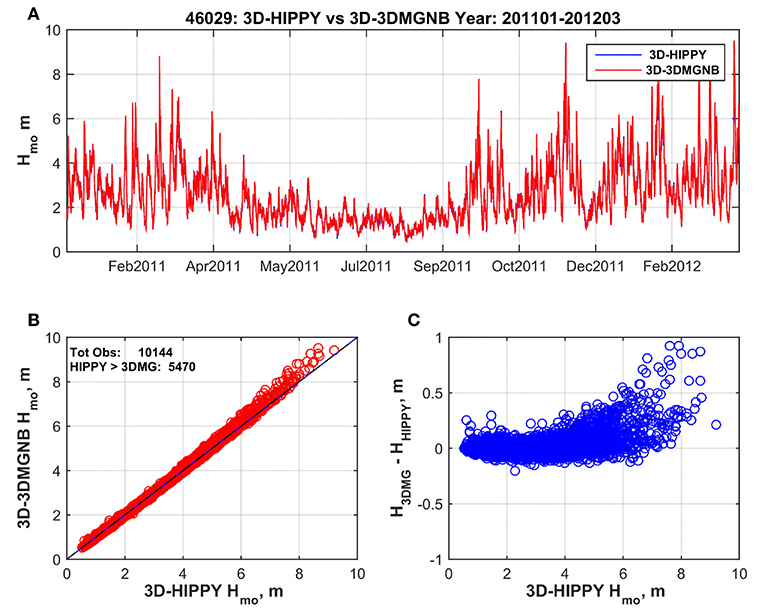
Figure 6. Differences in H s for two sensors, a strapped-down 3DMG accelerometer, and a gimballed HIPPY sensor, mounted on the same buoy NDBC buoy 46029 (Columbia River Bar, Oregon) in a water depth of 134 m. (A) Shows time series from january 2011 to February 2012. (B) Shows 3DMGNB against HIPPY. (C) Shows the difference between the two as a function of wave height.
As part of the DBCP Pilot Project on Wave Measurement Evaluation and Test (PP-WET; www.jcomm.info/WET), a field study evaluating the NOMAD (6N) was carried out in Monterey Bay from July 2015 through Oct 2018 (Jensen et al., 2015). The NOMAD buoy was equipped with five sensors, three from NDBC (Inclinometer, 3DMG-Motion Sensor, and a HIPPY™) and two from Canada (an MSC-WatchmanTM and Wave Module, and a TRIAXYS™ Next Wave II Directional Wave Sensor). In addition, a NDBC 3-m aluminum discus buoy (46042) containing their standard 3DMG motion sensor and a HIPPYTM sensor was deployed as well as a Datawell Directional Waverider™ (DWR) used as the relative reference for all evaluations (Luther et al., 2013). These sensors gave typical differences of 0.25 m for an average 2.5 m wave height (Jensen et al., 2015).
In most if not all evaluations over the past four decades we have relied on the significant wave height, peak, mean period and more recently the mean wave direction. These, other than the peak period Tp, are integral parameters. For example, the significant wave height for the analysis here is based on the integration of the frequency spectra given by Equation (4). The integration masks where differences may occur in the shape of the spectrum E(f).
WaveEval Tools, as described by Jensen et al. (2011) take a different approach. The four Fourier directional parameters are used to calculate the mean direction, spread, skewness and kurtosis (e.g., Kuik et al., 1988). Partitioning is performed on each discrete frequency band, and a discrete energy level. A bias and root mean square error percentage is determined from averaging the differences between two data sets. The result is a qualitative graphic displaying defined range of the per cent deviations. These techniques can provide useful information that is quantitative as well as qualitative reducing the assessment in directional properties to a reasonable number of products. Recently, two new methods have been proposed, evaluating frequency spectra (Dabbi et al., 2015) and correlating paired wave spectra (Collins et al., 2014).
There is no lack of trying to develop new methods to evaluate large spectral data sets to determine similarities, differences, quality or deficiencies in measurement to measurement systems, model to model results or model to measurements. However, we cling tightly to the bulk wave parameters because we know what they represent. For example two data sets produce a bias of 0.5 m out of 4 m. We know what that represents; we know how large a 0.5m Hs looks like. Now consider a difference in the frequency spectra of 10 m2s out of 125 m2s. The ratio is the same as in the case of the Hs, but what does it represent? That may be the only impediment holding the wave community back from progressing into the future. An intermediate solution is the use of partitions where we split a full spectrum into the single composing, and to a large extent independent, wave systems. Then the use of integral parameters makes more physical sense, and it is much more intuitive to mentally combine different and well defined wave systems coming together at the considered point.
Ensuring the quality of “First 5” data from present and future directional wave measurements would impact nearly every facet in the study of wind generated surface gravity waves from a physics based standpoint, to model improvements and daily performance of our weather prediction forecast centers. To have some quantifiable standard for all wave measurements would be highly beneficial to the user, and thus remove existing uncertainties, generally dismissed to the level where all data are at a uniform quality level, something far from the truth.
We should here mention other in situ measurement that may not comply with requirements but that are still used de facto, in particular when no other data source is available for delicate operations at sea. These include Ship-Borne Wave Recorders based on ship motions (e.g., Holliday et al., 2006; Nielsen, 2017) and X-band radar systems from Young et al. (1985) to more recent developments (e. g. Borge et al., 2004; Ma et al., 2015), and any combination of the two types of system. At present, very few datasets are available for the scientific community to make a detailed evaluation of the quality of these measurements. Their possible transmission on the Global Telecommunication System (GTS) of the WMO may promote a wider evaluation and use besides the need to have measurement at hand for real time decistion aid.
3.3. Satellite Remote Sensing
Routine measurements of sea states from satellites started with GEOSAT in 1985, with almost no interruption until today, except around 1990, as shown in Figure 7A. Over the years, different altimeters (solid bars in Figure 7A) supplied robust estimates of significant wave height (hereinafter Hs) and radar backscatter power related to the sea surface slope variance. Imaging radars have further given access to part of the directional wave spectrum (open boxes in Figure 7A).
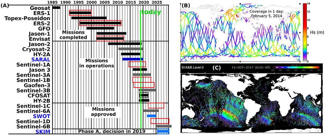
Figure 7. (A) Time coverage of satellite missions from 1985 to 2030, including nadir and near-nadir altimeters (solid bars), and missions monitoring ocean wave spectra (open boxes) using C-band Synthetic Aperture Radars (red), and real aperture radars in Ku-band (black) or Ka-band (blue). The lighter color (gray and blue) bars correspond to altimeters using Delay-Doppler processing. Source: CEOS database http://database.eohandbook.com/). (B) example of 1-day coverage for Hs measurements with 4 satellite altimeters (C) snapshot of a “fireworks” plot, the height (size of symbols) peak periods (colors), and directions (barbs) of swell partitions derived from Sentinel-1A and Sentinel-1B wave mode data. Such plots are produced routinely by CMEMS.
A new type of instrument, called a ‘wave spectrometer’ by Jackson et al. (1985), was successfully launched for the first time on a satellite, on 29 October 2018, with the SWIM instrument on CFOSAT (Hauser et al., 2017).
While robust and often quite unique to inform about extremes (Young, 1993; Quilfen et al., 2006, 2011), satellite altimeter measurements suffer from a limited spatial sampling, and can easily miss particular events, as evident from the example daily coverage in Figure 7B. This is less of a problem for wave mode data from synthetic aperture radars (SARs), but present measurements mostly provide reliable directional estimates for very long swells, i.e., with periods larger than 12 s (220 m wavelength). Compared to buoy measurements, satellites can still provide a larger volume of data, thereby sampling more extreme sea states (Hanafin et al., 2012), to further enable the tracking of wave-related extreme events across ocean basins Collard et al. (2009).
Clearly, the number of observations evolves as new satellites are launched and others are decommissioned (Figure 7A). When considering the altimeter data averaged at 1 Hz (about 7 km along-track), each satellite mission accounts for approximately 1 million observations per month as shown in Figure 8A. Given the along-track noise, mostly related to retracking issues, and sea state large scale correlations, these estimates cannot be considered independent. Moreover, the same region may often be sampled (in space and time) by two or more satellites, increasing the number of correlated observations.
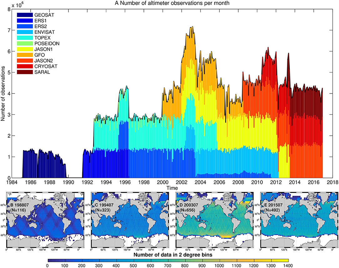
Figure 8. Number of radar altimetry 1 Hz observations per month (A). The lower panels show the number of observations in 2 × 2 longitude-latitude bins for July (B) 1988 (GEOSAT) (C) 1994 (ERS-1, Topex-Poseidon (D) 2003 (ERS-2, Envisat, Topex-Poseidon, Jason-1, GFO), and (E) 2015 (Jason-2, Cryosat-2, SARAL).
Most climate studies typically compute wave statistics by binning satellite observations into longitude-latitude regions such as 1–2° bins (Challenor et al., 1991; Young, 1999). Figures 8B–E shows the number of observations in 2° bins for representative time periods. Because the number of altimeter observations changes throughout the time period, the statistics computed from these data could be affected by sampling biases. This is critical for both low and high latitudes that have less observations. In addition, sampling biases affect most strongly the tails of the statistical distribution meaning both extremely small and large wave heights are observed with less precision than the average sea state.
For SAR wave mode data, sampling biases could be even more critical because the datasets were relatively sparse. Now with Sentinel-1A and Sentinel-1B in orbit, the number of observations per month has increased 20-fold from a median of 3 rather small imagettes per 2 × 2° bin each month with ERS-2, to 60 big imagettes today, which add up to 120,000 wave mode products per month. Also, the quality of the Sentinel-1 data is incomparable.
3.3.1. Significant Wave Height From Altimeters
Most of the altimeters sample repetitive tracks covering a full cycle in 10–35 days, with the 10-day repeat giving a large spacing between tracks. The working principle of satellite radar altimetry is quite simple. Pulses reflected by the sea surface at nadir are recorded as a function of time. This travel time gives the distance between the instrument and that surface. The main objective is to precisely track the distance between the instrument and the mean sea surface. Echoes reflected back from a wavy sea surface are registered in time and assembled as radar power signals called waveforms. These waveforms then mimic the cumulative distribution function associated to the wave amplitude statistics, such as shown on Figure 9A. A peaked waveform will correspond to low-sea state condition. At variance, broad waveforms correspond to high sea state conditions. Waveforms are usually averaged, and formed at a rate of 20-Hz, corresponding to a sampling of about 300 m along the satellite track. Over the ocean, altimeter waveforms are then further characterized by a rising and falling shape. The rising part, the leading edge, integrates echoes from the wave crests, initially located near the nadir center point of the footprint (e.g., Figure 9C), to the wave troughs. The falling part, the trailing edge, then integrates non-nadir backscattered echoes, located away from the nadir point. The Hs estimates are then derived from the extent of leading edge, and typically averaged every 7 km along the tracks (the so-called 1-Hz sampling rate). The accuracy on Hs estimates then depends, among other things, on the range resolution dr, which is dr = 0.30 m for Ka-band SARAL and dr = 48 cm for all other ku-band satellite altimeters, as the ka-band instrument operates with a larger radar frequency bandwidth. Although measurements are usually attributed to a precise longitude and latitude, the energy of the leading edge corresponds to a footprint reaching over 10 km in diameter and the value of Hs is in fact a weighted average over this footprint.
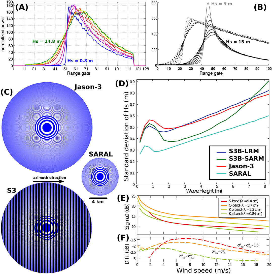
Figure 9. (A) Example of waveforms for a pass along the ascending track of SARAL/AltiKa on February 5, 2014, between 05:29:49 and 06:20:07 UTC. Each waveform shows the power measured by the radar as a function of time: time is discretized with intervals of 2 × 10⁻⁹ s corresponding to 30 cm range intervals usually called “range gates.” The corresponding wave heights are 0.8, 3.2, 4.6, 9.7, 10.7, 13.2, and 14.8 m. (B) averaged SARM (solid) and LRM (dashed) waveform from Sentinel-3 for Hs = 3,5,7,9,11,13 and 15 m, for cycle 23 orbit 349, on 25 October 2017 in the Pacific (C). Typical size of footprints on the ground for Jason-3, SARAL, and Sentinel-3, as limited by the radar antenna pattern. The rings with alternating blue and white filling, correspond to iso-range lines on a hypothetical flat surface. Only the first few rings are filled for readability. For Sentinel-3 the vertical bands show the azimuth resolution. (D) High-Frequency Noise on Hs, computed as Standard Deviation (SD) of high-frequency measurements within a 1-Hz along-track separation, with respect to Hs. Data are averaged for a full cycle of Jason-3, SARAL, Sentinel-3B LRM Mode (S-3B LRM, used in 13 days of cycle 10) and Sentinel-3B SAR Mode (S-3B SARM). (E) Backscatter strength (σ0) as a function of wind speed, and (F) differences for different radar frequencies, adapted from Quartly (2015), as authorized by Taylor & Francis.
A new generation of coherent radars can also use the phase of the radar echos. This allows a “SAR Mode” or “Delay-Doppler” processing that was pioneered with Cryosat-2 and is now used on Sentinel-3.
With delay only, the echoes are only distinguished by their time of arrival and each time window corresponds to an annular footprint on the sea surface (Figure 9C). In practice, most of the data contributing to the leading edge of the waveform come from a few range cells, that cover about half a significant wave height, i.e., for Hs = 2 m, the shape of the leading edge is determined by echoes from the first blue and white disks in Figure 9C. With the additional use of Doppler, the footprint can be separated in the along-track direction with “slices” (the black stripes in Figure 9C) that are typically 300 m wide (Raney, 1998; Scagliola, 2013). As a result, independent echoes acquired at different azimuth angles contain echoes from the same footprint “slice.” It is customary to stack together these echoes, with an incoherent sum in order to create a multi-looked waveform with a much better signal-to-noise ratio (Raney, 1998).
Also, both trailing and leading edges of Delay-Doppler waveforms are sensitive to Hs (Figure 9B, see also Ray et al., 2015). The shape of the waveform is sensitive to other sea state parameters, such as the wave orbital velocity, that could be estimated. Because of the beam-limited asymmetrical SAR altimetry footprint, ocean waves with a wavelength of a few 100 m (swell and extreme wind waves) may, depending upon their direction, no longer be fully imaged within the instrument ground cells and therefore produce a distorted waveform shape (Moreau et al., 2018).
The parameter estimation in satellite altimetry is performed by a fitting process called retracking. At present, two different theoretical waveform shapes are used to fit the measured LRM and SAR waveforms, namely the Brown-Hayne model (Brown, 1977; Hayne, 1980) and the SAMOSA model (Ray et al., 2015). In terms of precision, we show in Figure 9D a representation of noise computed as standard deviation of the high-frequency Hs estimations within a 1-Hz along-track separation, since the variation measured by the altimeter within 7 km is dominated by noise. The improvement of SAR altimetry compared with LRM altimetry is evident, except for at low and high sea states. Currently, the only Ka-band altimeter mission (SARAL, also known as AltiKa) has the lowest noise level, as shown in Figure 9D thanks to a smaller footprint and a higher number of pulses. The actual accuracy of these measurements is usually assessed by means of comparison with models and in situ data (e.g., Passaro et al., 2015; Sepulveda et al., 2015).
For coastal, near-ice or high resolution applications, altimetry is limited by the size of the footprint which can be contaminated by non-Gaussian surfaces such as land and ice, and the noise of the Hs estimates. Typically, LRM altimetry performs poorly at distances up to 20 km from the coast (Passaro et al., 2015). The smaller footprint of SAR altimetry and SARAL-Altika reduces this problem (Hithin et al., 2015; Dinardo et al., 2018). As for noise, it can be reduced by improving on the tracking methods (Passaro et al., 2015; Ardhuin et al., 2017a) and filtering the data (Quilfen et al., 2018). Other altimeter limitations involve low sea states, because the leading edge is poorly discretized, giving a large relative uncertainty in the estimation of Hs for Hs < 1 m (Smith and Scharroo, 2015), and rainy conditions, with stronger impacts as the altimeter frequency increases (e.g., Quilfen et al., 2006; Tournadre et al., 2015).
From these waveforms, the primary focus is the retrieval of the sea level, which is usually called “epoch” in that context, i.e., the time-distance between the instrument and the mean sea surface. As understood, backscatter echoes mostly correspond to specular local conditions as function of the surface wave elevation profiles. The epoch, and thus the derived sea level estimates, are then likely biased, as reflected radar signals are stronger in the troughs than near the crests of the waves. The bias is then written as , with h local surface elevation, σ local radar backscatter signals. This bias is then often corrected by directly using Hs, and the total mean backscatter coefficient , estimated from the waveform maximum.
3.3.2. Surface Roughness and Wind Speed From Altimeters
The other key parameter derived from the retracking process is the maximum amplitude of the radar echo, denoted by the normalized backscatter coefficient, σ0. This is primarily related to the statistics of surface slopes (Nouguier et al., 2016), usually summarized by the mean square slope (mss), which is primarily dependent upon the near surface wind speed at 10 m elevation, U10 (Cox and Munk, 1954; Bréon and Henriot, 2006). Yet, second-order effects, diffraction, curvature, and/or non-Gaussian effects can still be traced, especially when directly comparing coincident altimeter measurements performed with differing operating frequencies, i.e., C-band and Ku-band for TOPEX and the JASON instruments (Chapron et al., 1995; Elfouhaily et al., 1998; Tran et al., 2006).
Accordingly, there is no clear functional form that is appropriate to connect U10 to the mss, as the wind is not the only factor defining the mss. Although there is a very strong correspondence between wind speed and σ0, other factors certainly contribute to the measured backscatter. For instance, Vandemark et al. (1997) examined relationships between altimeter backscatter and the magnitude of near-surface wind and friction velocities, with improved agreements found after correcting 10-m winds for both surface current and atmospheric stability. More importantly, Elfouhaily et al. (1998) and Gourrion et al. (2002), and Golubkin et al. (2015) showed that σ0 strongly responds to the sea state degree of development. Using the Hs altimeter estimates as an indicator of the sea state degree of development, wind estimates can be improved, in particular now that the noise of Hs and σ0 estimates can be reduced following Sandwell and Smith (2005) and Quilfen et al. (2018). This is limited to not too young sea states, otherwise the same pair of measurements can correspond to two pairs of sea states (U10, Hs) with very different wave ages (Farjami et al., 2016).
As an alternative analysis strategy, it has been demonstrated that with increasing wind speeds, the dual-frequency data provide a measurement more directly linked to the short-scale surface roughness (Chapron et al., 1995), which in turn is associated with the local surface wind stress (Elfouhaily et al., 1998), and gas transfer (Frew et al., 2007). The dual-frequency data also highlight the effect of rain on the perceived signal (Quartly et al., 1996).
Finally, Vandemark et al. (2016) demonstrated that sea surface temperature also modulates σ0 through its effect on the emissivity of water, and Quartly (2010) showed that, for the TOPEX and Jason satellites, there are unexplained oscillations in recorded σ0 associated with changing solar illumination of the spacecraft. Most of these factors are ignored in current operational wind speed algorithms.
We note that there is significant uncertainty about the absolute calibration of σ0 for all past and present altimeters. Efforts to produce an absolute calibration for σ0 from Envisat using calibrated on-ground transponders still had an uncertainty of 1 dB (Pierdicca et al., 2013), whereas the required tolerance for climate studies necessitates knowing the drift to better than 0.03 dB/decade. Thus, in practice, all current wind speed algorithms are empirical, based on matching up altimeter observations of σ0 with a host of meteorological buoys and instruments on ships or other platforms of opportunity.
Without absolute calibration, considerable efforts are thus directed to align σ0 observations from one mission to a predecessor on the same orbit, the integrity of the climate record rests on the buoys and models used for long-term monitoring of instrument performance. In particular, there is not even an agreed universal scale for σ0 data, with the values recorded by two Ku-band altimeters differing by an offset of more than 2 dB. Furthermore, as mentioned above, there is no simple adjustment between normalized backscatter observations at one radar frequency with those at another (Figures 9E–F), because each is responding to a different scale length of sea surface roughness as illustrated by Figures 9E,F. Since there have been more than 30 years of Ku-band and C-band altimetry, the launch of SARAL operating only at Ka-band, necessitated a new specific effort to produce relevant wind speed algorithms (Lillibridge et al., 2014; Quartly, 2015).
Global analyses of the joint altimeter measurements of Hs and σ0 related U10 show that the majority of the ocean is dominated by swell (Chen et al., 2002). These combined metocean records then further invite other parameters to be developed either theoretically or empirically, such as pseudo wave age (Glazman and Pilorz, 1990) and wave period (Gommenginger et al., 2003; Mackay et al., 2008).
3.3.3. 2D Wave Spectra Monitoring With Synthetic Aperture Radars and Other Imagery
Synthetic aperture radars (SARs) are coherent microwave radars that measure the sea surface roughness and Doppler at very high resolution, using the Doppler frequency to achieve a high resolution in the satellite flight direction (known as azimuth), of the order of 5 m depending on the instrument acquisition mode. Remote sensing with SAR has then been generally focused on land (ground deformation, subsidence …) and sea ice applications (Kwok et al., 1990). Indeed, such a fine resolution capability can only be achieved provided the target can be considered as frozen during the integration time of the order of 0.5 s. In practice, over the ocean, orbital motions of high frequency waves cannot be neglected and can strongly degrade the azimuth resolution to a couple of 100 m, depending on the sea state (Kerbaol et al., 1998; Stopa et al., 2015). Accordingly, the SAR azimuth response mirrors the probability distribution of the radial velocity component of the scatters and causes the azimuth resolution to be proportional to the root mean square orbital motions of the high frequency waves. Wave components with wavelengths larger than the azimuth cutoff have constructive velocity bunching while waves with shorter wavelengths have destructive velocity bunching and are strongly distorted. Therefore, swells are often well resolved by SAR and are consistent with in-situ buoy observations (Collard et al., 2009).
Still, over oceans, SARs are unique in providing all-weather very high resolution imagery of a wide variety of oceanic and atmospheric phenomena. Mature ocean applications include the measurement of winds at high resolution (e.g., Mouche et al., 2017), and ocean waves. In particular, the ERS-1, ERS-2, Envisat, Sentinel 1 and Gaofen-3 satellite include a default “wave mode” for acquisition over the oceans that allows the routine mapping of wave properties over large scales (Hasselmann et al., 2012).
In the open ocean, the processes that explain the formation of wave patterns in a SAR image, such as Figure 10, are fairly complex and can be quite non-linear (Hasselmann et al., 1985; Tucker, 1985; Alpers and Bruening, 1986; Holt, 1988; Hasselmann and Hasselmann, 1991). Yet, the unique capability to possibly capture directional wave properties, in particular the part associated with long swells (Lehner, 1984) means that a sparse coverage of the ocean is enough to observe full swell fields, as shown in Figure 7C (Collard et al., 2009).
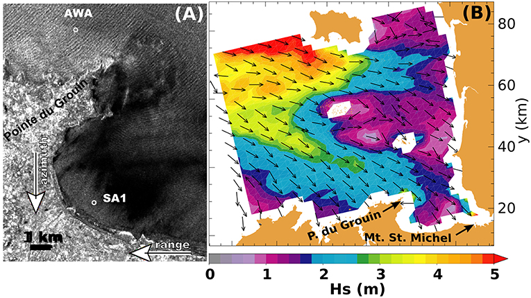
Figure 10. (A) extract from an Envisat IW mode image, March 2003 (see Collard et al., 2005) and (B) map of wave heights and mean direction estimated from the Single Look Complex image.
A wide range of methods have been developed to retrieve wave information from SAR imagery, with important contributions from Engen and Johnsen (1995) who introduced multi-look formation from Single Look Complex image that allows one to reduce the noise in the spectra and lift the 180° ambiguity in wave propagation direction. Both aspects are used in the quasi-linear spectrum retrieval algorithms (Chapron et al., 2001b; Johnsen and Collard, 2004) that form the basis of the ESA level-2 products for wave mode data. In practice the ambiguity removal may fail to pick the right direction, which explains why a few arrows point west instead of east in Figure 10. As mentioned above, the precision of SAR wave parameters has been assessed from 2D spectra comparison between buoy observations and SAR spectra (Collard et al., 2009). Precision is low for environmental conditions with strong distortion from the azimuth cutoff effect (e.g., storms). However, in the far field, emitted swells are well captured, leading to consistently observe basin-scale swell patterns by using the space-time consistency swells (e.g., the fireworks in Figure 7C, see also Collard et al., 2009).
To complement retrieval algorithms, empirical methods have been proposed for SAR to more directly estimate Hs from σ0 mean and normalized variance estimates. At first, an original technique, called CWAVE, was developed for ERS-2 by Schulz-Stellenfleth et al. (2007). Specifically, CWAVE uses σ0, the normalized variance of radar cross section, and 20 other orthogonal statistics computed from the image modulation spectrum to empirically estimate Hs. CWAVE was re-calibrated for ENVISAT (Li et al., 2011) and Sentinel-1 (Stopa and Mouche, 2017). As retreived, Hs exceeding 9 m are consistent with numerical models and radar altimeter estimates in extra-tropical storms and tropical cyclones (Stopa and Mouche, 2017). Therefore, the SAR technology can estimate waves in environments where the standard approaches to estimate directional wave spectral property from the image spectrum typically perform poorly. CWAVE is adaptable to estimate other sea state parameters such as wave energy and wave period, but the precision is reduced compared to Hs (Schulz-Stellenfleth et al., 2007; Stopa and Mouche, 2017).
Finally, optical imagery, even if they cannot offer a full global monitoring for all seasons due to particular observation constraints (cloud cover and sun zenith), are unique in their resolving capability with, for example all coastal areas covered by Landsat and Sentinel 2A and 2B satellites. Sentinel-2 capability to precisely estimate the full directional wave spectrum has been demonstrated by Kudryavtsev et al. (2017), and is further discussed by Villas Bôas et al. (2019). This unique capability is taking advantage of the different parallax angles between the 12 adjacent detectors used to cover the 280 km swath at 10 m resolution. This slightly different viewing geometry is used to estimate the transfer function between brightness variations and slope variations. Additional information on the wave dispersion and current velocity can then be quite uniquely extracted from the different sensing time (up to about 2 s) of the same point on ground by different channels within each detector, having also slightly different viewing angles. These enhanced capabilities certainly open new possibilities to combine different satellite measurements (including SAR and altimeter measurements) and possibly provide validation opportunities for upper ocean motions, including surface currents and its gradients, and waves. Recent airborne demonstrations by Yurovskaya et al. (2018) show that daylight sea state monitoring with drones is already feasible.
3.4. Other Observations: Microseisms
Among the many other measurements that contain a signature of sea state, a special mention should be given to the background noise recorded everywhere on Earth, and known as microseisms.
Microseisms are the dominant signal in seismometers. The strongest microseisms have periods around 4 to 10 s, and are generated when waves with similar frequency travel in opposing directions (Longuet-Higgins, 1950; Hasselmann, 1963) and microseisms have a frequency doubled compared to that of the ocean waves. This generation of seismic waves is particularly amplified in deep water and vanishes in shallow water (Ardhuin and Herbers, 2013), with vertical ground motions of a few micrometers that correspond to seismic Rayleigh waves. The sea states that are most effective for generating microseisms can be classified is three broad classes, and include, is order of magnitude, the generally broad directional spectrum at high frequency, the effect of coastal reflection, and the collision of two wave systems from different storms (Ardhuin et al., 2011).
The signal around 7 s is so clear, that seismic stations were set-up in the late 1940s to detect and track hurricanes (Gutemberg, 1947), and were used on the U.S. west coast in the 1970s to measure ocean waves (Zopf et al., 1976). With ocean buoys and satellites available, using microseisms for sea state application may sound outdated. Still, seismic records are unique in their sensitivity, being able to pick-up swell fore-runners of amplitudes under 0.1 m (Husson et al., 2012), and covering many regions of the world for which, before CFOSAT, there was no measurement of wind sea spectra (e.g., Barruol et al., 2006).
Following Zopf et al. (1976), and using data from the Berkeley seismic station (BKS) in California, Bromirski et al. (1999) showed how one may reconstruct a time series of ocean wave spectra from the seismic spectra of a nearby land station. This was further explored by Ardhuin et al. (2012), as shown in Figure 11A for the year 2008, using a power law relation estimated from the first 20 days of the year (shaded gray).
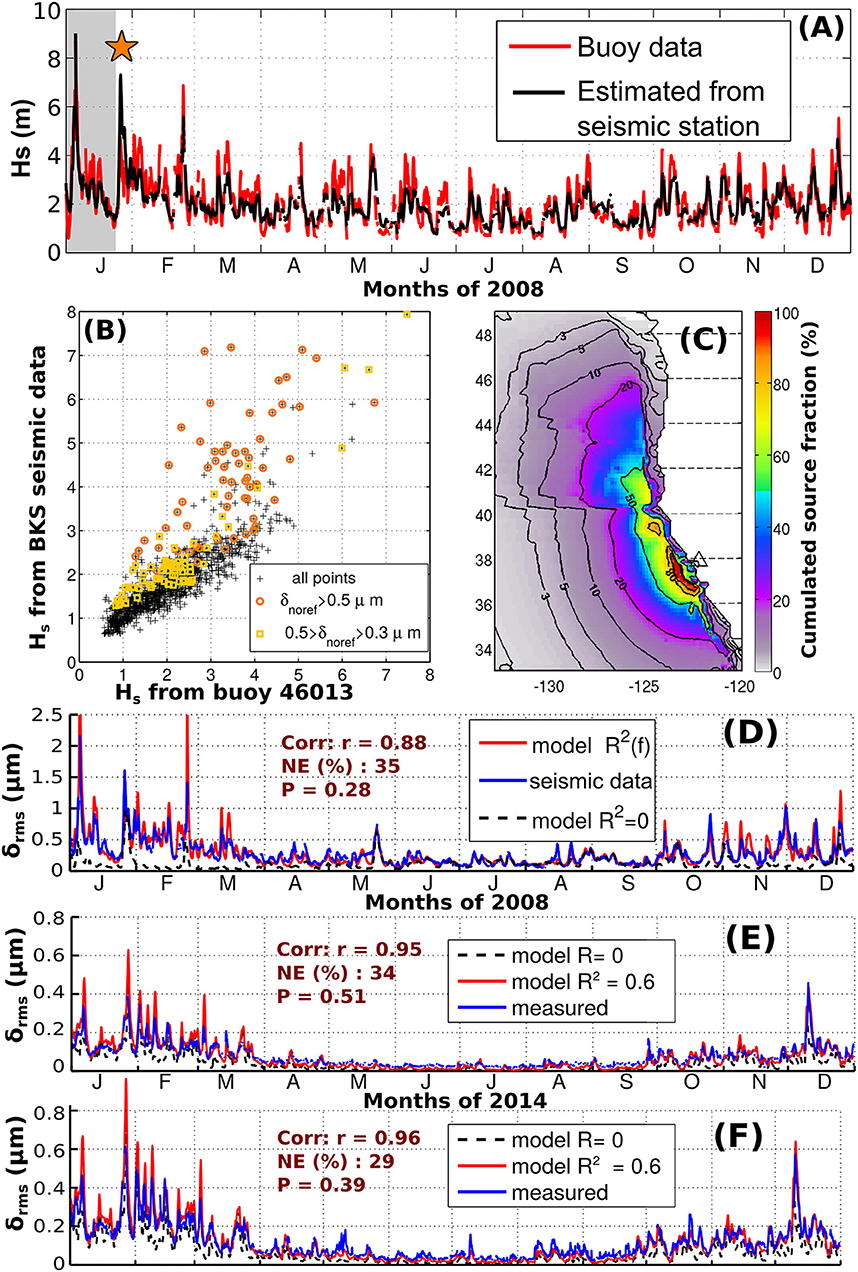
Figure 11. (A) Measured wave heights at buoy 46013 and estimates from the BKS seismic station. The star marks a particular event on January 26 with microseisms generated by oposing wave trains from two distinct storms. (B) Correlation between measured and estimated wave heights, highlighting the outliers unrelated to coastal reflections (C) Average spatial distribution of microseism sources recorded at the BKS seismic station (triangle). (D–F): modeled and measured microseism amplitude at stations BKS, station 4 of the Grafenberg array (Germany), and Uccle (Belgium). Model results are shown with or without coastal reflection to give a sense of the uncertainty of the simulation and of the importance of the wave energy reflection coefficient, which is set here at 6, 12, and 24% for continents and large islands, islands smaller than 50 km, and icebergs, respectively.
Although there is a clear correlation between wave heights and microseism amplitude, the relation between the two varies because microseism amplitudes are the product of the amplitude of the wave trains traveling in opposing directions. When, the opposing waves are generated by coastal reflection, this gives one particular relation, but when the opposing waves are due to two uncorrelated wave systems, this typically gives a very strong noise, with a very weak correlation to the wave height (e.g., Obrebski et al., 2012; Butler and Aucan, 2018). One may use a wave model with or without wave reflection at the shoreline to probe this effect, and clearly, all the outliers in Figure 11B are caused by events unrelated to shoreline reflection.
Another important question when estimating wave parameters from microseisms is the location of the sources in the ocean. In the case of California, a direct modeling of the seismic sources suggests that 50% of the sources, on average, are located withing a 800 km band of ocean along the California coast, with water depths over 300 m. This is highly dependent on seismic propagation and attenuation, and other sites, such as Hawaii or the Tuamotus are sensitive to sources over a much wider region. It is thus difficult in general to estimate wave height at a single location from a single seismic station, and one may use multiple stations (Möllhoff and Bean, 2016) or a coherent processing of station arrays that can use seismic body waves instead of surface Rayleigh waves to locate the seismic sources (Gerstoft et al., 2006; Obrebski et al., 2013; Meschede et al., 2017).
Instead of trying to invert the signal, one may use a forward model from wave spectra to the seismic signal. This is made difficult by the poor knowledge of wave reflection at the shore and seismic wave propagation for these periods (Ying et al., 2010; Gualtieri et al., 2015). Still, the correlation between modeled and measured seismic ground displacement is usually very high, suggesting that seismic data could be assimilated to correct the wave model, its forcing, or the seismic propagation model. Figures 11E,F show observed and modeld microseisms at the Grafenberg array in the south of Germany, with numerical data available since 1976, and the Uccle station in Brussels, Belgium, where instruments have been recording since 1898.
One of the greatest interests in microseisms arises from the long term time series that can be obtained. Bernard (1981, 1990) made early attempts at studying the wave climate from microseisms, analyzing data between 1910 and 1975 from 12 seismic stations, mostly located around the North Atlantic. His 2-year averaged relative microseim amplitude oscillated between 0.8 and 1.2 without any clear trend but near-decadal oscillations. Bernard attributed these oscillations to an influence of the 11-year sun cycle on the storms, where a modern reader would rather see the pattern of the North Atlantic Oscillation. More recently, Grevemeyer et al. (2000) estimated a “microseism index” from the Hamburg seismic station, which increased 4-fold between 1955 and 1995. They linked that trend to a trend in wave heights measured at Seven Stones (off the southwest coast of the UK), which increased by 20% from 1960 to 1985. Such trends are not compatible with other seismic data analyses (e.g., Aster et al., 2008), highlighting the difficulty of estimating stable amplitudes from different instruments spanning over a century of seismic monitoring.
Besides the main microseism peak, Other signals are recorded at longer periods, which are well explained by the interaction of waves with a sloping bottom, and microseisms are generated at the same frequency as the waves, in the primary microseism band, 10–20 s (Ardhuin, 2018), and in the hum band, 30–300 s (see Deen et al., 2018). These other bands can also be used to constrain sea states, including infragravity waves.
4. Future of Sea State Measurements
4.1. In situ Observations
Here we focus on the major in situ wave measurement centers, defined as those transmitting to the Global Telecommunication System (GTS) of the WMO in real time, i.e. within 1–3 h from the measurement. Data that do not make it on to the GTS do not exist for most applications, we will come back to this. These centers have faced with an increase in operation and maintenance costs, not to mention an increase in vandalism. Meeting the needs of users such as Numerical Weather Prediction Centers, researchers and developers of new wave modeling technologies, continuation of long-term records in the investigation of climate trends, has become a challenge.
Unfortunately, support for network expansion, upgrades to existing platforms to measure directional information, has so far been deemed by the agencies responsible for wave measurement to be too costly, in spite of the previous recommendations (Swail et al., 2009). Instead, these agencies have focused on trying to reduce costs in various ways.
Fortunately, and very timely, technological advances since OceanObs'09 with respect to wave measurement have been extremely prolific, especially with regard to high-quality sensors, but also with platforms and real-time transmission. Rather than simply decommissioning existing assets (i.e., reducing the number of buoys), there has been a transition toward the replacement of large buoys (e.g., 12 m, 10 m, NOMADs) and migration of 3 m aluminum hulls to smaller foam-based buoys with even smaller discus hulls with diameters 1.8, 2.3, 2.4, and 2.1 m (Hall et al., 2018). These new platforms minimize the need for large vessels, and increase the number of buoys able to be transported during a scheduled cruise. Wave measurement sensors have migrated to small computer chip systems (Teng and Bouchard, 2005; Teng et al., 2009; Riley et al., 2011). With the advent of the smaller hulls, improved battery packs, less power required and new compact sensor packages, changes are being made to the super-structure configuration of NDBC buoys as shown in Figure 12. Also, Datawell is now manufacturing its buoys with different hull diameters. While the smaller hulls are easier to deploy and better suited for shorter wave periods, it should be noted that these buoys have different responses (Datawell, 2014).
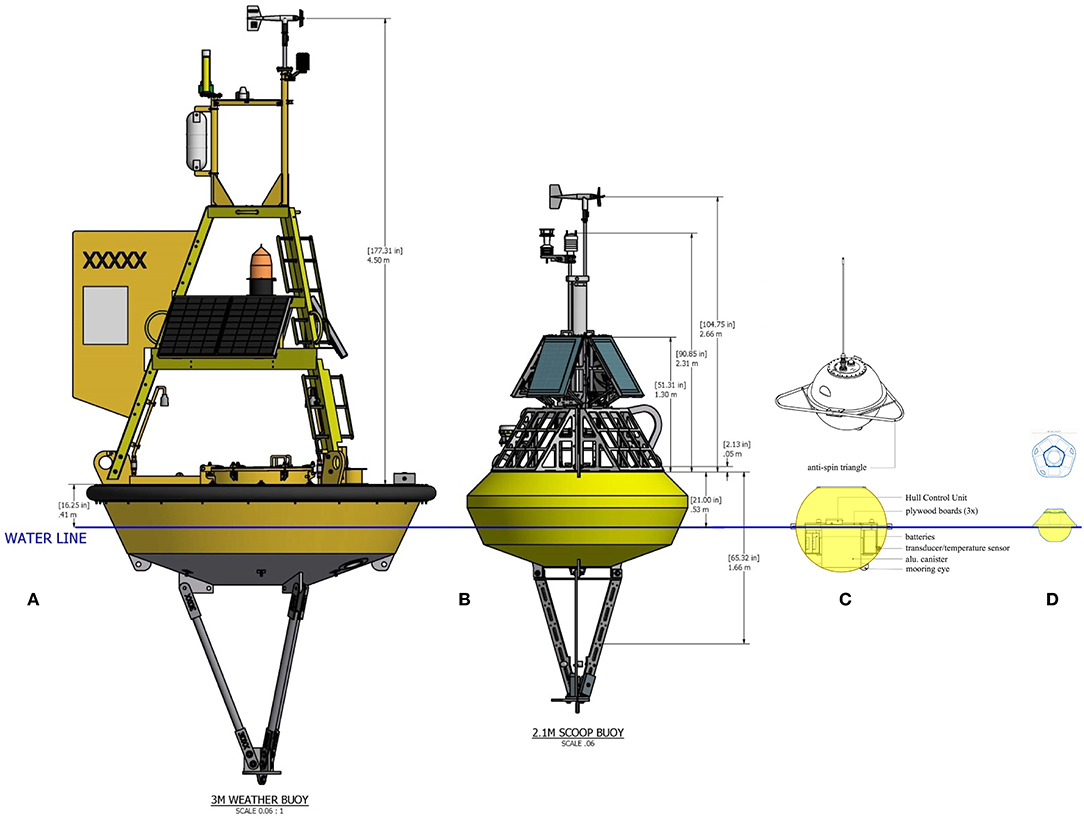
Figure 12. Schematics of existing and planned super-structures of NDBC moored buoys measuring waves, (credit Eric Gay, NDBC). (A) is the standard design of 3-m discus buoys (Steele et al., 1992) pictured in Figure 1A, (B) is the new SCOOP design with a 2.1 m diameter that is replacing many buoys. The 3-m diameter SCOOP is pictured in Figure 1B. For reference, (C) is the schematic for the Mark 4 Datawell waverider with a 0.9 m hull diameter, drawn to scale, and (D) is the schematic of a Spotter buoy made by Spoondrift, following the developments of Herbers et al. (2012).
We note that the motion sensor in many of new NDBC configurations such as in Figure 12B is located well above the mean water level, whereas historically (Figure 12A) that sensor is placed inside the hull at the water level. Foam composition buoy hulls are much lighter than NDBC's standard 3m aluminum hull. As previously mentioned, the RAO (transfer function of the buoy motion to the free surface) has to be quantified for the hull weight, super-structure modification, and also the sensor location. If properly formulated and evaluated through laboratory and field testing the quality in the new buoy systems should be as accurate as has been found historically.
Also, GPS velocity measurements have been used to estimate the wave conditions from small buoy systems (Vries et al., 2003; Herbers et al., 2012; Thomson, 2012; Reverdin et al., 2013; Centurioni et al., 2018, 2019; Guimaraes et al., 2018). The buoy velocities are determined in a fixed frame of reference from the external GPS signals eliminating the need for calibration of an on-board motion-sensor or compass. This reduces the size and cost, so that it can be mounted in very small hulls. One of the drawbacks of the GPS measurement approach is that the communication relies on a satellite link that could be disrupted by large wave conditions or submerged from breaking waves. Despite this shortcoming, these systems would have the potential for the expansion of the world's wave measurement array at limited cost.
Wave measurements from the small GPS drifters can have a significant impact on our ability to observe the world's oceans that would parallel existing and new generation satellite-based remote sensing systems. The equipment of just 10% of the existing drifter buoys (cyan symbols in Figure 13B) with high-quality directional wave measurement systems, would have a great impact for Numerical Weather Prediction, the evaluation of numerical wave models, ship routing, and early warning for tropical cyclone or remote swell impacts that are a dominant flooding hazard in some regions (Lefèvre, 2009; Hoeke et al., 2013). A similar extension of wave measurement to moored buoys in the tropics would also greatly contribute to the understanding of air-sea fluxes (Cravatte et al., 2016). Further, there are substantial gaps in the Coastal Buoy Network (red symbols in Figure 13B, see Figure 13A for those reporting wave measurements on the GTS). Although, the addition of many more coastal stations is doubtful in the near future, the amount of data could easily be doubled if the organizations in charge of collecting wave data could transmit it over the GTS.
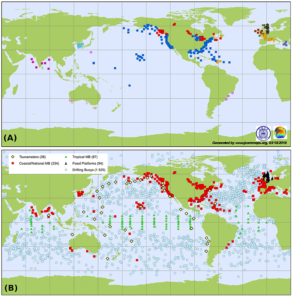
Figure 13. (A) Fixed locations for wave data transmitted via JCOMM, with different colors for different countries, and (B) location of surface instruments transmitting data through the GTS as part of the Data Buoy Cooperation Panel (DBCP) which could all be equipped with cheap wave sensors, source http://www.jcommops.org/dbcp/network/maps.html.
The proliferation of low cost, high-quality directional wave sensors in the past few years, coupled with the increased use of smaller hulls has greatly reduced the cost of wave measuring systems, so that the entire moored buoy networks could eventually be transformed to the “First-5” directional measurement capability at a lower cost than existing networks. New technologies are continually being developed which may also come into play over the next decade, including the possibility of high-quality measurements from gliders (Daniel et al., 2011), stereo video (Fedele et al., 2013; Benetazzo et al., 2017), or lidar scanning (McNinch, 2007). These last two techniques have already proven very useful for wave research and may find a broader community of users with the continued decrease of processing and instrument costs.
4.2. Remote Sensing
As listed on Figure 7, the very large increase in the number and capabilities of new satellite missions that we have seen over the past decade will likely continue, with very important innovations in terms of instruments and concepts. Starting with altimeters, the revolution of Delay-Doppler altimetry is ongoing, and these have yet to be fully exploited, probably allowing the estimation of more parameters, including a more direct measurement of the mean period Tm0,2. The Surface Water Ocean Topography mission (SWOT, Morrow et al., 2019) is due for launch in 2021. It is primarily designed to measure the water level of sea, rivers and lakes but it is very sensitive to waves, and will thus add particular estimates of wave orbital velocity and wave height across its 120 km wide swath. SWOT is in fact a SAR with near-nadir incidences that will provide unprecedented measurements of surface currents and their small scale gradients, which are very important for the forcing of wave models or the interpretation of wave measurements (see Figure 2).
Among the novelties that was brought by the European Copernicus program are the long term commitment to continue series of SAR imagery with wave mode data, the use of a constellation of two C-band SAR (Sentinel-1 A and B instead of one with respect to previous European mission) and the modification of the wave mode for an improved sampling of swells (two incidence angles instead of one with respect to previous European mission). This means that the extension of the Sentinel-1 mission is already planned and agreed between the European Commission and the European Space Agency with Sentinel-1C and -1D launches planned for 2022 and 2023. They will ensure the continuity of Copernicus service at least until the end of 2030. With Sentinel-1 mission, waves from SAR have also been formally integrated into the Marine Service (CMEMS).
This includes Level-2 and higher level products such as the “Fireworks”. Relying on the self-consistency of a given swell field, the swell measurements are analyzed at the ocean basin scale to flag outliers and provide quality-controlled swell fields. Overall, about 50% of the Level-2 swell measurements are filtered. The consistency between these measurements and the unqualified Level-2 swell measurements is verified using cross-overs between neighboring swell observations. Swell measurements propagated up to 48h are co-located (maximum distance <200 km) and their peak direction and peak wavelength compared, thus providing several thousands of co-located points in a single month, over open ocean regions not sampled by in situ measurements.
Such high level products also allows one to combine Sentinel-1 A and Sentinel-1 B products providing inter-calibrated swell measurements. In this context, the recent launch of CFOSAT, will provide new directional ocean wave spectra measurements at global scale. “Fireworks” analysis will quickly provide inter-comparisons with Sentinel-1 mission data, leading to a possible inter-calibration step with the goal of using together CFOSAT and Sentinel-1 data to feed the Level-3 and Level-4 Copernicus waves products.
As a matter of fact, in addition of their complexity (2D spectrum of ocean swell + swell partitions to be compared to significant wave height from altimeters), the quality of the SAR spectra is still poorly documented in the Level-2 products and consequently these products are very little used. But the proper calibration (e.g., Li et al., 2018) and the foreseen developments to include a robust quality flag (for each swell partition) in the Level-2 products should foster a wider use of these data that provide a unique view with a great coverage of global swell fields (Figure 8C). Also, more efforts on the larger images using Sentinel-1 and other missions is leading to interesting coastal applications (e.g., Rikka et al., 2018). Possible future constellation of SARs may greatly enrich this capability.
In ice-covered waters, high frequency waves that are usually responsible for nonlinear distortion are attenuated quickly (Wadhams et al., 1988). Therefore, wave signatures on SAR imagery in sea ice are mainly due to velocity bunching (Vachon et al., 1993; Ardhuin et al., 2015). Standard techniques, like the quasi-linear approach (Chapron et al., 2001a), are not sufficient to capture the nonlinearity of the wave features on the SAR imagery. By only considering the velocity bunching mechanism, maps of orbital wave motions can be inverted, giving access to the full E(k, θ) wave spectrum (Ardhuin et al., 2017a). Further development of this wave retrieval, with the handling of ice features (Stopa et al., 2018b), is opening great opportunities for applications, with the systematic analysis and investigation of wave attenuation in ice (Ardhuin et al., 2018; Stopa et al., 2018a; see Figures 14A–F).
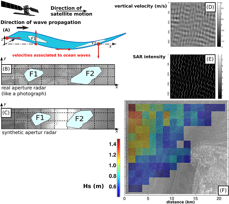
Figure 14. (A) schematic illustrating the geometry of SAR observation and vertical velocities at the surface. (B) Example of a real aperture radar scene stretched into (C) a SAR scene due to varying vertical velocities in the azimuth direction: actual features such as ice floes F1 and F2 appear displaced in the azimuth (x) direction. (D) example of simulated vertical velocity map due to two swell trains propagating at right angles and (E) simulated SAR intensity in the case of a sea surface with uniform σ0. (F) Intensity map (gray shades) observed by Sentinel-1A in Southern Ocean sea ice on 03/05/2016 at 10:55:53 UTC, and overlaid map of Hs in color obtained by inverting the SAR intensity pattern into a vertical velocity map. This example is further discussed in Stopa et al. (2018b).
Finally, CFOSAT is producing its first wave spectra down to 70 m wavelength (typically a period of 6.7 s), this is a clear demonstration of the power of real aperture radars, in Ku-band in the case of SWIM on CFOSAT, for monitoring waves in the open ocean. Using a Ka-band radar instead makes it possible to resolve shorter components, probably 20 m (3.6 s), with smaller footprints and a wider swath. This is one of the goals of the Surface KInematics Multiscale (SKIM) mission (Ardhuin et al., 2018), which is designed to measure both currents and wave spectra, and is presently undergoing a detailed study for a possible launch in 2025.
Other imaging methods, using constellations of radar or optical sensors will probably further expand our capabilities to monitor sea state. Optical imagery is unique in providing unambiguous information about whitecaps and their distributions, which are important for applications ranging from navigation safety to upper ocean mixing, surface drift (Rascle and Ardhuin, 2009), and air-sea fluxes.
The future of sea state monitoring is also in its past. Considering both the new and historical data, important evolution in processing algorithms are expected. In particular, for altimeters, alternative retracking solutions have emerged to improve the data quality and quantity for satellite altimetry at the coast (Cipollini et al., 2017). One of the most successful techniques consists of selecting only a portion of the waveform, in order to avoid spurious contamination by the trailing edge (Deng and Featherstone, 2005). While the main focus was on the range retrieval, some of these studies have included specific performance analysis for Hs (Passaro et al., 2015; Roscher et al., 2017, 2018; Dinardo et al., 2018). The use of different fitting methods can also lead to a much lower noise in Hs estimates (Ardhuin et al., 2017b). All of these new methods can be combined with adaptive filters to separate tracker noise from geophysical signals (Quilfen et al., 2018), as illustrated in Figure 2.
5. Recommendations
We list here a few practical things that could make future sea state observation more useful and valuable.
5.1. In situ Observational Systems
There is a clear requirement for more high-quality directional wave spectral data in all parts of the global ocean. With the development of new low cost sensors and cheaper platforms, transition of non-directional wave measurement sites to directional capability should be pursued.
With the continued development of new wave measurement systems, as well as for the historical measurements that make up the climate record, test and evaluation remains critical to the understanding of the differences found, as originally stated in Swail et al. (2009). Testing should consider spatially differing wave climates, and temporally span multiple years (inter-annual variability). The evaluation procedure should include integral wave parameters, frequency, frequency-directional estimates, hierarchy evaluation techniques, and to establish a set of standardized metrics defining the quality of the wave measurement system.
A global network of directional spectral wave drifters, supplemented as feasible by targeted campaigns such as deploying wave drifters in advance of large storms including hurricanes, should be implemented over the next decade. This network may include new platforms, including ships of opportunity (Nielsen et al., 2019), once their errors are known. Adding many doubtful data should not be thought as a replacement for high quality measurements that are particularly needed for long term climate monitoring and statistics on extreme events.
5.2. Historical Data and Metadata
As equally important to high-quality directional wave measurements, self-describing metadata is necessary to define all characteristics associated with the data. The world's wave measurement data providers are addressing this issue with existing information. However, large gaps still exist in the metadata records from historical deployments. Without this valuable information, there will be a continuation of misrepresenting long-term wave measurement records as identified by Gemmrich et al. (2011). In addition, the metadata records for all in-situ wave measurements need to be archived and made easily accesible to any user requiring the information. Ideally, these wave metadata would be archived with the actual measured data in a centralized Global Data Assembly Center (GDAC). GDACs have been created for other data sets (e.g., Pinardi et al., 2019), but not as yet for waves.
5.3. Data Sharing and Distribution
To serve the full range of users, any in situ wave observation network should accurately resolve the details of the directional spectral wave field as well as providing the standard integrated parameters. It is strongly recommended that all directional wave measuring devices should reliably estimate the “First 5” standard parameters, and that these spectral parameters be distributed in an easy-to-use format, possibly following the example set by the Coastal Data Information Program (CDIP). We appreciate the sharing of long time series such as the 39-year Aqua Alta data (Pomaro et al., 2018). However, we are missing a common repository or portal for accessing multiple data sets from multiple sites.
5.4. Open Processing, Re-processing, and Algorithms
Given the complexity of all the steps necessary to get from the raw data to a final product, we recommend that algorithms and associated ancillary data be fully documented and published, at least in technical reports. This particulary include any calibration (e.g., for the power in altimeter waveforms).
In the case of remote sensing data (true for altimeter and SAR), the number of available sensors, the co-existence of different algorithms and alternative processing methods invite to produce homogeneous (format) and (inter-calibrated) data sets covering the whole period since the beginning of the earth observation area. New sensors such as CFOSAT for wave spectra, concept missions like SKIM or recent SAR altimeters, all with new and specific capabilities, also advocate for a strategy to build a common and tractable database that will ease the use of the remote sensing data for science applications by non-experts.
5.5. Leveraging Acquisition Capability of SARs
The acquisition capabilities of satellites is under-used today for the monitoring of extreme events. For example, high winds can now be estimated from Sentinel-1 satellites when acquired in cross-polarization (Mouche et al., 2017). A systematic acquisition over severe storms, and a similar measurement of waves in ice (Ardhuin et al., 2017c) could provide critical information on sea states and associated parameters in situations of practical use as well as high value for research.
5.6. Combining Data and Models
Wave assimilation methods have been developed in many fields, but has long been limited in the case of ocean waves due to the fact buoys were close to the coast, hence having a impact on a very short time, or that altimeters only measured wave heights with a limited improvement on spectra, and in particular swells in long-range forecasts. Now that more drifting buoys are becoming available, and that new satellites are measuring more of the spectrum, there is room to fully exploit the space-time correlation structures of swells (e.g., Delpey, 2012) as provided by models and data, both for the optimization of initial conditions and the estimate of model parameters. We note the recent work by Crosby et al. (2017) who optimized the offshore directional wave spectrum at the boundary of a coastal wave model, and similar work could be developed to optimize the wind, current and sea ice parameters that are part of the forcing functions of wave models.
6. Summary and Conclusions
The past decade has lead to an amazing increase in the quantity and quality of sea state data collected and distributed, in particular from satellites and in seismic records. These new data are revealing new features of the oceanic wave field, and in particular the importance of ocean currents in defining the small scale variability. As a result, new observation systems should take into account this variability, which is why we propose a new set of requirements for sea state monitoring (Table 1). In the short term, reaching these requirements will require a proper combination of in situ and satellite data with numerical wave models. Besides, this also requires a better knowledge of winds, currents, and sea ice properties, to which new remote sensing efforts such as SKIM (Ardhuin et al., 2018) can contribute, but which can also benefit from a more creative use of existing data (e.g., Quilfen et al., 2018; Rio and Santoleri, 2018).
At the same time, the in situ observation networks have matured and gone through important changes in terms of sensors use and data distribution, with, unfortunately, the metadata often lagging behind. Now that human activities are being more and more exposed to marine hazards due to sea level rise, coastal land subsidence, and intensification of extreme storms, a careful work of documenting and understanding wave climate and its variability is required. This is calling for continued support and funding for basic data collection and quality control, including the archival of metadata, and new research on analysis methods combining all sources of data variability, in particular for the extreme events. Given the relatively short record of buoy and satellite data, other sources of information have probably an important role to play. These include visual observations from ships and seismic records, but the methods to combine all these data and reduce the uncertainties on trends to acceptable levels have yet to be refined, tested and validated.
Author Contributions
GQ and MP contributed the initial version of sections on satellite altimeters, JS and IY wrote the sections on trends, JJ, VS, and FA wrote the section on requirements, RJ and VS contributed the initial versions of sections on in situ data, AM, JS, and FA wrote the sections on the other sensors (SARs, CFOSAT, SKIM, seismometers). All authors contributed to the final editing.
Funding
FA, GQ, and MP are supported by ESA under the Sea State CCI project. Additional support from CNES and ANR grants for ISblue (ANR-17-EURE-0015) LabexMER (ANR-10-LABX-19), and MIMOSA (ANR-14-CE01-0012).
Conflict of Interest Statement
The authors declare that the research was conducted in the absence of any commercial or financial relationships that could be construed as a potential conflict of interest.
Acknowledgments
We acknowledge the acquisition, processing and dissemination of sea state data by many organizations including NASA, CNES, ESA, EUMETSAT, NOAA, CDIP, Environment and Climate Change Canada, the Copernicus Marine Environment Monitoring Service, JCOMM, GOOS, and its regional organizations.
Footnotes
1. ^This particular convention, with direction from is commonly used in coastal applications. Some other applications prefer to use the direction to.
References
Allan, J., and Komar, P. (2000). Are ocean wave heights increasing in the eastern north pacific? Eos 81, 561. doi: 10.1029/eo081i047p00561-01
Allen, P. A., and Hoffman, P. F. (2005). Extreme winds and waves in the aftermath of a neoproterozoic glaciation. Nature 433, 123–127.
Alpers, W., and Bruening, C. (1986). On the relative importance of motion related contributions to the SAR imaging mechanism of ocean surface waves. IEEE Trans. Geosci. Remote Sens. 24, 873–885
Andrews, D. G., and McIntyre, M. E. (1978). On wave action and its relatives. J. Fluid Mech. 89, 647–664.
Ardhuin, F. (2018). Large scale forces under surface gravity waves at a wavy bottom: a mechanism for the generation of primary microseisms. Geophys. Res. Lett. 45, 8173–8181. doi: 10.1029/2018GL078855
Ardhuin, F., Aksenov, Y., Benetazzo, A., Bertino, L., Brandt, P., Caubet, E., et al. (2018). Measuring currents, ice drift, and waves from space: the sea surface kinematics multiscale monitoring (SKIM) concept. Ocean Sci. 14, 337–354. doi: 10.5194/os-2017-65
Ardhuin, F., Balanche, A., Stutzmann, E., and Obrebski, M. (2012). From seismic noise to ocean wave parameters: general methods and validation. J. Geophys. Res. 117, C05002. doi: 10.1029/2011JC007449
Ardhuin, F., Chapron, B., and Collard, F. (2009). Observation of swell dissipation across oceans. Geophys. Res. Lett. 36, L06607. doi: 10.1029/2008GL037030
Ardhuin, F., Chapron, B., Collard, F., Smith, M., Stopa, J., Thomson, J., et al. (2017a). Measuring ocean waves in sea ice using SAR imagery: a quasi-deterministic approach evaluated with Sentinel-1 and in situ data. Remote sens. Environ. 189, 211–222. doi: 10.1016/j.rse.2016.11.024
Ardhuin, F., Collard, F., Chapron, B., Girard-Ardhuin, F., Guitton, G., Mouche, A., et al. (2015). Estimates of ocean wave heights and attenuation in sea ice using the sar wave mode on Sentinel-1A. Geophys. Res. Lett. 42, 2317–2325. doi: 10.1002/2014GL062940
Ardhuin, F., Drake, T. G., and Herbers, T. H. C. (2002). Observations of wave-generated vortex ripples on the North Carolina continental shelf. J. Geophys. Res. 107, 7-1–7-14. doi: 10.1029/2001JC000986
Ardhuin, F., and Herbers, T. H. C. (2013). Noise generation in the solid earth, oceans and atmosphere, from nonlinear interacting surface gravity waves in finite depth. J. Fluid Mech. 716, 316–348. doi: 10.1017/jfm.2012.548
Ardhuin, F., Rascle, N., Chapron, B., Gula, J., Molemaker, J., Gille, S. T., et al. (2017b). Small scale currents have large effects on wind wave heights. J. Geophys. Res. 122, 4500–4517. doi: 10.1002/2016JC012413
Ardhuin, F., Rogers, E., Babanin, A., Filipot, J.-F., Magne, R., Roland, A., et al. (2010). Semi-empirical dissipation source functions for wind-wave models: part I, definition, calibration and validation. J. Phys. Oceanogr. 40, 1917–1941. doi: 10.1175/2010JPO4324.1
Ardhuin, F., Stutzmann, E., Schimmel, M., and Mangeney, A. (2011). Ocean wave sources of seismic noise. J. Geophys. Res. 116, C09004. doi: 10.1029/2011JC006952
Ardhuin, F., Suzuki, N., McWilliams, J. C., and Aiki, N. (2017c). Comments on “a combined derivation of the integrated and vertically resolved, coupled wave-current equations”. J. Phys. Oceanogr. 47, 2377–2385. doi: 10.1175/JPO-D-17-0065.1
Ashton, A., Murray, A. B., and Arnault, O. (2001). Formation of coastline features by large-scale instabilities induced by high-angle waves. Natue 414, 296–299. doi: 10.1038/35104541
Aster, R. C., McNamara, D. E., and Bromirski, P. D. (2008). Multidecadal climate-induced variability in microseisms. Seis. Res. Lett. 79, 194–202
Autret, R., Dodet, G., Fichaut, B., Suanez, S., David, L., Leckler, F., et al. (2016). A comprehensive hydro-geomorphic study of cliff-top storm deposits on Banneg island during winter 2013-2014. Mar. Geol. 382, 37–55. doi: 10.1016/j.margeo.2016.09.014
Barruol, G., Reymond, D., Fontaine, F. R., Hyvernaud, O., Maurer, V., and Maamaatuaiahutapu, K. (2006). Characterizing swells in the southern pacific from seismic and infrasonic noise analyses. Geophys. J. Int. 164, 516–542. doi: 10.1111/j.1365-246X.2006.02871.x
Belward, A. (2016). The Global Observing System for Climate: Implementation Needs. Technical Report GCOS-200, World Meteorological Organization
Bender, L. C. III., N. L. Guinasso, N. L. Jr., Walpert, J. N., and Howden, S. D. (2010). A comparison of methods for determining significant wave heights applied to a 3-m discus buoy during hurricane Katrina. J. Atmos. Ocean Technol. 27, 1012–1028. doi: 10.1175/2010JTECHO724.1
Benetazzo, A., Ardhuin, F., Bergamasco, F., Cavaleri, L., Guimarães, P. V., Schwendeman, M., et al. (2017). On the shape and likelihood of oceanic rogue waves. Sci. Rep. 7, 8276. doi: 10.1038/s41598-017-07704-9
Bernard, P. (1981). Sur l'existence et l'amplitude de la variation undécennale des microséismes météorologiques. C. R. Acad. Sci. Paris 293, 687–689.
Bernard, P. (1990). Historical sketch of microseisms from past to future. Phys. Earth Planetary Interiors 63, 145–150. doi: 10.1016/0031-9201(90)90013-N
Bertelli, T. (1872). Osservazioni sui piccoli movimenti dei pendoli in relazione ad alcuni fenomeni meteorologiche. Boll. Meteorol. Osserv. Coll. Roma 9, 10.
Bidlot, J.-R. (2016). Twenty-One Years of Waveforecast Verification. Technical Report. ECMWF Newsletter No. 150 – Winter 2016/17, ECMWF, Reading. doi: 10.18442/ECMWF-NL-201610
Bitner-Gregersen, E., Cramer, E., and Korbijin, F. (1995). “Environmental description for long-term load response of ship structures,” in Proceedings of the 2004 ISOPE Conference, (Toulon: ISOPE), 221–226.
Borge, J. C. N., Rodriguez, G. R., Hessner, K., and Gonzalez, P. I. (2004). Inversion of marine radar images for surface wave analysis. J. Atmos. Ocean Technol. 21, 1291–1300. doi: 10.1175/1520-0426(2004)021<1291:IOMRIF>2.0.CO;2
Bouchette, F., Schuster, M., Ghienne, J.-F., Denamiel, C., Roquin, C., Moussa, A., et al. (2010). Hydrodynamics in holocene lake mega-chad. Q. Res. 73, 226–236. doi: 10.1016/j.yqres.2009.10.010
Bréon, F. M., and Henriot, N. (2006). Spaceborne observations of ocean glint reflectance and modeling of wave slope distributions. J. Geophys. Res. 111, C0605. doi: 10.1029/2005JC003343
Bromirski, P. D., Flick, R. E., and Graham, N. (1999). Ocean wave height determined from inland seismometer data: implications for investigating wave climate changes in the NE Pacific. J. Geophys. Res. 104, 20753–20766
Brown, G. S. (1977). The average impulse response of a rough surface and its applications. IEEE J. Oceanic Eng. 2, 67–63. doi: 10.1109/JOE.1977.1145328
Butler, R., and Aucan, J. (2018). Multisensor, microseismic observations of a hurricane transit near the ALOHA cabled observatory. J. Geophys. Res. 123, 3027–2046. doi: 10.1002/2017JB014885
Caires, S., and Sterl, A. (2005). 100-year return value estimates for ocean wind speed and significant wave height from the ERA-40 data. J. Clim. 18, 1032–1048. doi: 10.1175/JCLI-3312.1
Cartwright, D. E., and Longuet-Higgins, M. S. (1956). The statistical distribution of the maxima of a random function. Proc. R. Soc. Lond. A 237, 212–232.
Centurioni, L., Braasch, L., Di Lauro, E., Contestabile, P., De Leo, F. R C., et al. (2018). “A new strategic wave measurement station off naples port main breakwater,” in Proceedings of 35th Conference on Coastal Engineering, November (Antalya: ASCE).
Centurioni, L., Lumpkin, R., Brassington, G., Chao, Y., Charpentier, E., Corlett, G., et al. (2019). Multidisciplinary global in-situ observations of essential climate and ocean variables at the air-sea interface in support of climate variability and change studies and to improve weather forecasting, pollution, hazard and maritime safety assessments. Front. Mar. Sci.
Challenor, P., Foale, S., and Webb, D. J. (1991). Seasonal changes in the global wave climate measured by the GEOSAT altimeter. Int. J. Remote Sens. 11, 2205–2213.
Chapron, B., Johnsen, H., and Garello, R. (2001a). Wave and wind retrieval from SAR images of the ocean. Ann. Telecommun. 56, 682–699. doi: 10.1007/BF02995562
Chapron, B., Katsaros, K., Elfouhaily, T., and Vandemark, D. (1995). “A note on relationships between sea surface roughness and altimeter backscatter,” in Air-Water Gas Transfer, Selected Papers From the Third International Symposium on Air-Water Gas Transfer, eds B. Jäne and E. C. Monahan (Heidelberg), 869–878.
Chapron, B., Vandemark, D., Elfouhaily, T., Thompson, D. R., Gaspar, P., and Labroue, S. (2001b). Altimeter sea state bias: a new look at global range error estimates. Geophys. Res. Lett. 28, 3947–3950. doi: 10.1029/2001GL013346
Chawla, A., Spindler, D. M., and Tolman, H. L. (2013). Validation of a thirty year wave hindcast using the climate forecast system reanalysis winds. Ocean Model. 73, 189–206. doi: 10.1016/j.ocemod.2012.07.005
Chen, G., Chapron, B., Ezraty, R., and Vandemark, D. (2002). A global view of swell and wind sea climate in the ocean by satellite altimeter and scatterometer. J. Atmos. Ocean Technol. 19, 1849–1859. doi: 10.1175/1520-0426(2002)019<1849:AGVOSA>2.0.CO;2
Cipollini, P., Benveniste, J., Birol, F., Fernandes, M., Obligis, E., Passaro, M., et al. (2017). “Chapter 11 Satellite altimetry in coastal regions,” in Satellite Altimetry Over oceans and Land Surfaces, eds D. Stammer and A. Cazenave (New York, NY: CRC Press), 38.
Collard, F., Ardhuin, F., and Chapron, B. (2005). Extraction of coastal ocean wave fields from SAR images. IEEE J. Oceanic Eng. 30, 526–533. doi: 10.1109/JOE.2005.857503
Collard, F., Ardhuin, F., and Chapron, B. (2009). Monitoring and analysis of ocean swell fields using a spaceborne SAR: a new method for routine observations. J. Geophys. Res. 114, C07023. doi: 10.1029/2008JC005215
Collins, C. O. III., Lund, B., Waseda, T., and Graber, H. C. (2014). On recording sea surface elevation with accelerometer buoys: lessons from ITOP (2010). Ocean Dyn. 64, 895–904. doi: 10.1007/s10236-014-0732-7
Cox, C., and Munk, W. (1954). Measurement of the roughness of the sea surface from photographs of the sun's glitter. J. Opt. Soc. Am. 44, 838–850. doi: 10.1364/josa.44.000838
Cox, R., Zentner, D. B., Kirchner, B. J., and Cook, M. S. (2016). Boulder ridges on the Aran Islands (Ireland): Recent movements caused by storm waves, not tsunamis. J. Geol. 120, 249–272. doi: 10.1086/664787
Cravatte, S., Kessler, W. S., Smith, N., and Wijffels, S. E. and Contributing Authors (2016). First Report of TPOS. Technical Report 215, GOOS.
Cronin, M. F., Gentemann, C. L., Edson, J., Ueki, I., Bourassa, M., Brown, S., et al. (2019). Air-sea fluxes with a focus on heat and momentum. Front. Marine Sci.
Crosby, S. C., Cornuelle, B. D., O'Reilly, W. C., and Guza, R. T. (2017). Assimilating global wave model predictions and deep-water wave observations in nearshore swell predictions. J. Atmos. Ocean Technol. 34, 1823–1836. doi: 10.1175/JTECH-D-17-0003.1
Dabbi, E. P., Haigh, I. D., Lambkin, D., Hernon, J., Williams, J. J., and Nicholls, R. J. (2015). Beyond significant wave height: A new approach for validating spectral wave models. Coastal Eng. 100, 11–25. doi: 10.1016/j.coastaleng.2015.03.007
Daniel, T., Manley, J., and Trenaman, N. (2011). The wave glider: enabling a new approach to persistent ocean observation and research. Ocean Dyn. 61, 1509–1520. doi: 10.1007/s10236-011-0408-5
Datawell (2014). Datawell-High Frequency Heave Resonance. Technical Report. Available online at: https://www.youtube.com/watch?v=OlrCKTnrhbQ.
Dee, D. P., Uppala, S. M., Simmons, A. J., Berrisford, P., Poli, P., Kobayashi, S., et al. (2011). The era-interim reanalysis: configuration and performance of the data assimilation system. Q. J. R. Meteorol. Soc. 137, 553–597. doi: 10.1002/qj.828
Deen, M., Stutzmann, E., and Ardhuin, F. (2018). The earth's hum variations from a global model and seismic recordings around the Indian ocean. Geochem. Geophys. Geosyst. 19, 4006–4020. doi: 10.1029/2018GC007478
Delpey, M. (2012). Etude de la Dispersion Horizontale en Zone Littorale Sous l'effet de la Circulation Tridimensionnelle forcée par les Vagues. Ph.D. thesis, Université Européenne de Bretagne, Ecole doctorale des Sciences de la Mer (Brest).
Deng, X., and Featherstone, W. E. (2005). A coastal retracking system for satellite radar altimeter waveforms: application to ERS-2 around Australia. J. Geophys. Res. 111, C06012. doi: 10.1029/2005JC003039
Dinardo, S., Fenoglio-Marc, L., Buchhaupt, C., Becker, M., Scharroo, R., Fernandes, M. J., et al. (2018). Coastal sar and plrm altimetry in german bight and west baltic sea. Adv. Space Res. 62, 1371–1404. doi: 10.1016/j.asr.2017.12.018
Dodet, G., Leckler, F., Sous, D., Ardhuin, F., Filipot, J., and Suanez, S. (2018). Wave runup over steep rocky cliffs. J. Geophys. Res. 123, 7185–7205. doi: 10.1029/2018JC013967
Durrant, T. H., Greenslade, D. J. M., and Simmonds, I. (2010). Validation of Jason-1 and Envisat remotely sensed wave heights. J. Atmos. Ocean Technol. 26, 123–134. doi: 10.1175/2008jtecho598.1
Elfouhaily, T., Vandemark, D., Gourrion, J., and Chapron, B. (1998). Estimation of wind stress using dual-frequency TOPEX data. J. Geophys. Res. 103, 25101–25108.
Engen, G., and Johnsen, H. (1995). Sar-ocean wave inversion using image cross spectra. IEEE Trans. Geosci. Remote Sens. 33, 4.
England, M. H., McGregor, S., Spence, P., Meehl, G. A., Timmermann, A., Cai, W., et al. (2014). Recent intensification of wind-driven circulation in the Pacific and the ongoing warming hiatus. Nat. Clim. Change 75, 222–227. doi: 10.1038/NCLIMATE2106
Fan, Y., Lin, S.-J., Held, I. M., Yu, Z., and Tolman, H. L. (2012). Global ocean surface wave simulation using a coupled atmosphere–wave model. J. Clim. 25, 6233–6252. doi: 10.1175/jcli-d-11-00621.1
Farjami, H., Golubkina, P., and Chapron, B. (2016). Impact of the sea state on altimeter measurements in coastal regions. Remote Sens. Lett. 7, 935–944. doi: 10.1080/2150704X.2016.1201224
Fedele, F., Benetazzo, A., Gallego, G., Shih, P.-C., Yezzi, A., Barbariol, F., et al. (2013). Space-time measurements of oceanic sea states. Ocean Model. 70, 103–115. doi: 10.1016/j.ocemod.2013.01.001
Fedele, F., and Tayfun, M. A. (2007). Wave height distributions and nonlinear effects. Ocean Eng. 34, 1631–1649. doi: 10.1016/j.oceaneng.2006.11.006
Freeman, E., Woodruff, S. D., Worley, S. J., Kent, S. J. L. C., Angel, W. E., Berry, D. I., et al. (2017). ICOADS release 3.0: a major update to the historical marine climate record. Int. J. Climatol. 37, 2211–2232. doi: 10.1002/joc.4775
Frew, N. M., Glover, D. M., Bock, E. J., and McCue, S. J. (2007). A new approach to estimation of global air-sea gas transfer velocity fields using dual-frequency altimeter backscatter. J. Geophys. Res. 112, C11003. doi: 10.1029/2006JC003819
Fyfe, J. C., Meehl, G. A., England, M. H., Mann, M. E., Santer, B. D., Flato, G. M., et al. (2014). Making sense of the early-2000s warming slowdown. Nat. Clim. Change 75, 224–228. doi: 10.1038/nclimate2938
Gallet, B., and Young, W. R. (2014). Refraction of swell by surface currents. J. Mar. Res. 72, 105–126. doi: 10.1357/002224014813758959
Gemmrich, J., and Garrett, C. (2012). The signature of inertial and tidal currents in offshore wave records. J. Phys. Oceanogr. 42, 1051–1056. doi: 10.1175/JPO-D-12-043.1
Gemmrich, J., Thomas, B., and Bouchard, R. (2011). Observational changes and trends in northeast Pacific wave records. Geophys. Res. Lett. 38, L22601. doi: 10.1029/2011GL049518
Gerling, T. W. (1992). Partitioning sequences and arrays of directional ocean wave spectra into component wave systems. J. Atmos. Ocean Technol. 9, 444–458.
Gerstoft, P., Fehler, M. C., and Sabra, K. G. (2006). When Katrina hit California. Geophys. Res. Lett. 33, L17308. doi: 10.1029/2006GL027270
Glazman, R. E., and Pilorz, S. H. (1990). Effects of sea maturity on satellite altimeter measurements. J. Geophys. Res. 95, 2857–2870. doi: 10.1029/jc095ic03p02857
Golubkin, P. A., Chapron, B., and Kudryavtsev, V. N. (2015). Wind waves in the arctic seas: envisat and AltiKa data analysis. Mar. Geol. 38, 289–298. doi: 10.1080/01490419.2014.990592
Gommenginger, C. P., Srokosz, M. A., Challenor, P. G., and Cotton, P. D. (2003). Measuring ocean wave period with satellite altimeters: a simple empirical model. Geophys. Res. Lett. 30, 2150. doi: 10.1029/2003GL017743
Gourrion, J., Vandemark, D., Bailey, S., and Chapron, B. (2002). Investigation of C-band altimeter cross section dependence on wind speed and sea state. Can. J. Remote Sens. 28, 484–489. doi: 10.5589/m02-046
Gower, J. F. R. (2002). Temperature, wind and wave climatologies, and trends from marine meteorological buoys in the northeast pacific. J. Clim. 15, 3709–3718. doi: 10.1175/1520-0442(2002)015<3709:twawca>2.0.co;2
Grevemeyer, I., Herber, R., and Essen, H.-H. (2000). Microseismological evidence for a changing wave climate in the northeast Atlantic Ocean. Nature 408, 349–351. doi: 10.1038/35042558
Grigorieva, V. G., and Badulin, S. I. (2016). Wind wave characteristics based on visual observations and satellite altimetry. Oceanology 56, 19–24. doi: 10.1134/S0001437016010045
Gualtieri, L., Stutzmann, E., Capdeville, Y., Farra, V., Mangeney, A., and Morelli, A. (2015). On the shaping factors of the secondary microseismic wavefield. J. Geophys. Res. 120, 1–22. doi: 10.1002/2015JB012157
Guimaraes, P. V., Ardhuin, F., Sutherland, P., Accensi, M., Hamon, M., Pérignon, Y., et al. (2018). A Surface KInematics Buoy (SKIB) for wave-current interactions studies. Ocean Sci. Discuss. 14, 1449–1460. doi: 10.5194/os-2018-45
Gulev, S. K., and Grigorieva, V. (2006). Variability of the winter wind waves and swell in the north atlantic and north pacific as revealed by the voluntary observing ship data. J. Clim. 19, 5667–5685. doi: 10.1175/JCLI3936.1
Gulev, S. K., Grigorieva, V., Sterl, A., and Woolf, D. (2003). Assessment of the reliability of wave observations from voluntary observing ships: insights from the validation of a global wind wave climatology based on voluntary observing ship data. J. Geophys. Res. 108, 3236. doi: 10.1029/2002JC001437
Gutemberg, B. (1947). Microseisms and weather forecasting. J. Meteorol. 4, 21–28. doi: 10.1175/1520-0469(1947)004<0021:MAWF>2.0.CO%3B2
Guymer, T. H., Quartly, G. D., and Srokosz, M. A. (1995). The effects of rain on ERS-1 radar altimeter data. J. Atmos. Ocean Technol. 12, 1229–1247. doi: 10.1175/1520-0426(1995)012<1229:TEOROR>2.0.CO;2
Hall, C., Bouchard, R. H., Riley, R., Stewart, R., Wang, D., and DiNapoli, S. (2018). Emerging National Data Buoy Center (NDBC) Wave Systems. Technical Report Presentation at DBCP-34 meeting, 22 October, Cape Town, South Africa, NOAA National Data Buoy Center (NDBC), Stennis Space Center, MS.
Hanafin, J., Quilfen, Y., Ardhuin, F., Sienkiewicz, J., Queffeulou, P., Obrebski, M., et al. (2012). Phenomenal sea states and swell radiation: a comprehensive analysis of the 12-16 February 2011 North Atlantic storms. Bull. Amer. Meterol. Soc. 93, 1825–1832. doi: 10.1175/BAMS-D-11-00128.1
Hande, L. B., Siems, S. T., and Manton, M. J. (2012). Observed trends in wind speed over the southern ocean. Geophys. Res. Lett. 39, L11802. doi: 10.1029/2012GL051734
Hanson, J. L., and Phillips, O. M. (2001). Automated analysis of ocean surface directional wave spectra. J. Atmos. Ocean Technol. 18, 277–293. doi: 10.1175/1520-0426(2001)018<0277:AAOOSD>2.0.CO;2
Hasselmann, K. (1963). A statistical analysis of the generation of microseisms. Rev. of Geophys. 1, 177–210.
Hasselmann, K., Chapron, B., Aouf, L., Ardhuin, F., Collard, F., Engen, G., et al. (2012). “The ERS SAR wave mode: a breakthrough in global ocean wave observations,” in ERS Missions: 20 Years of Observing Earth (European Space Agency; Noordwijk), 165–198.
Hasselmann, K., and Hasselmann, S. (1991). On the nonlinear mapping of an ocean wave spectrum into a synthetic aperture radar image spectrum and its inversion. J. Geophys. Res. 96, 10713–10729.
Hasselmann, K., Raney, R. K., Plant, W. J., Alpers, W., Shuchman, R. A., Lyzenga, D. R., et al. (1985). Theory of synthetic aperture radar ocean imaging: a MARSEN view. J. Geophys. Res. 90, 4659–4686.
Hauser, D., Tison, C., Amiot, T., Delaye, L., Corcoral, N., and Castillan, P. (2017). SWIM: The first spaceborne wave scatterometer. IEEE Trans. Geosci. Remote Sens. 55, 3000–3014. doi: 10.1109/TGRS.2017.2658672
Hayne, G. (1980). Radar altimeter mean return waveforms from near-normal-incidence ocean surface scattering. IEEE Trans. Antennas Propagat. 28, 687–692. doi: 10.1109/tap.1980.1142398
Hemer, M. A., Church, J. A., and Hunter, J. R. (2009). Variability and trends in the directional wave climate of the southern hemisphere. Int. J. Climatol. 33, L06604. doi: 10.1002/joc.1900
Hemer, M. A., Katzfey, J., and Trenham, C. E. (2013). Global dynamical projections of surface ocean wave climate for a future high greenhouse gas emission scenario. Ocean Model. 70, 221–245. doi: 10.1016/j.ocemod.2012.09.008
Herbers, T. H. C., Janssen, T. T., Colbert, D. B., and MacMahan, J. H. (2012). Observing ocean surface waves with gps-tracked buoys. J. Atmos. Ocean Technol. 29, 944–959. doi: 10.1175/JTECH-D-11-00128.1
Hersbach, H., and Dee, D. (2016). ERA-5 reanalysis is in production. Technical Report ECMWF Newsletter No. 147 – Spring 2016, ECMWF, (Reading).
Hithin, N. K., Remya, P. G., Nair, T. M. B., Harikumar, R., Kumar, R., and Nayak, S. (2015). Validation and intercomparison of SARAL/AltiKa and PISTACH-derived coastal wave heights using in-situ measurements. IEEE J. Selec. Topics App. Earth Obs. Remote Sens. 8, 4120–4129. doi: 10.1109/JSTARS.2015.2418251
Hoeke, R. K., McInnesa, K. L., Kruger, J. C., McNaught, R. J., Hunter, J. R., and Smithers, S. G. (2013). Widespread inundation of Pacific islands triggered by distant-source wind-waves. Glob. Plan. Change 108, 128–138. doi: 10.1016/j.gloplacha.2013.06.006
Holliday, N. P., Yelland, M. J., Pascal, R., Swail, V. R., Taylor, P. K., Griffiths, C. R., et al. (2006). Were extreme waves in the Rockall trough the largest ever recorded? Geophys. Res. Lett. 33, L05613. doi: 10.1029/2005GL025238
Holman, R. A., and Stanley, J. (2007). The history and technical capabilities of argus. Coastal Eng. 54, 477–491. doi: 10.1016/j.coastaleng.2007.01.003
Holt, B. (1988). Introduction: studies of ocean wave spectra from the shuttle imaging radar-b experiment. J. Geophys. Res. 93, 15365–15366.
Husson, R., Ardhuin, F., Chapron, B., Collard, F., and Balanche, A. (2012). Swells throughout the pacific: a combined view using the global seismic network and Envisat's wave mode asar data. Geophys. Res. Lett. 39, L15609. doi: 10.1029/2012GL052334
IACS (2001). Standard wave data. Technical Report Rec. Number 34, International Association of Classification Societies.
IAHR Working Group on Wave Generation and Analysis (1989). List of sea-state parameters. J. Waterway Port Coast. Ocean Eng. 115, 793–807.
Jackson, F. C., Walton, W. T., and Peng, C. Y. (1985). A comparison of in situ and airborne radar observations of ocean wave directionality. J. Geophys. Res. 90, 1005–1018.
Janssen, P. A. E. M. (2009). On some consequences of the canonical transformation in the Hamiltonian theory of water waves. J. Fluid Mech. 637, 1–44. doi: 10.21957/2lqx2y8rc
Jensen, R., Swail, V., Buchard, R., Riley, R., Hesser, T., Blaseckie, M., et al. (2015). “Field laboratory for ocean sea state investigation and experimentation: FLOSSIE intra-measurement evaluation of 6n wave buoy systems,” in Proceedings of the 14th International Workshop on Wave Hindcasting and Forecasting & 5th Coastal Hazard Symposium (Key West, FL).
Jensen, R., Swail, V., Lee, B., and O'Reilly, W. (2011). “Wave measurement evaluation and testing,” in Proceedings of the 12th International Workshop on Wave Hindcasting and Forecasting (Kohala Coast, HI).
Johnsen, H., and Collard, F. (2004). ASAR Wave Mode Processing - Validation of Reprocessing Upgrade. Technical report for ESA-ESRIN under contract 17376/03/I-OL, 168, NORUT.
Kennedy, A. B., Mori, N., Zhang, Y., Yasuda, T., Chen, S.-E., Tajima, Y., et al. (2016). Observations and modeling of coastal boulder transport and loading during super typhoon haiyan. Coastal Eng. Japan 58, 1640004. doi: 10.1142/S0578563416400040
Kerbaol, V., Chapron, B., and Vachon, P. (1998). Analysis of ERS-1/2 synthetic aperture radar wave mode imagettes. J. Geophys. Res. 103, 7833–7846.
Krogstad, H. E. (2005). “Conventional analysis of wave measurement arrays,” in Measuring and Analysing the Directional Spectra of Ocean Waves, eds D. Hauser, K. Kahma, H. E. Krogstad, S. Lehner, J. A. J. Monbaliu, and L. R. Wyatt (Luxembourg city: Office for Official Publications of the European Communities). 56–71.
Krogstad, H. E., Wolf, J., Thompson, S. P., and Wyatt, L. R. (1999). Methods for intercomparison of wave measurements. Coastal Eng. 37, 235–257.
Kudryavtsev, V., Yurovskaya, M., Chapron, B., Collard, F., and Donlon, C. (2017). Sun glitter imagery of surface waves. part 1: directional spectrum retrieval and validation. J. Geophys. Res. 122, 369–1383. doi: 10.1002/2016JC012425
Kuik, A. J., van Vledder, G. P., and Holthuijsen, L. H. (1988). A method for the routine analysis of pitch-and-roll buoy wave data. J. Phys. Oceanogr. 18, 1020–1034.
Kwok, R., Curlander, J. C., McConnell, R., and Pang, S. (1990). An icemotion tracking system at the Alaska SAR facility. IEEE J. Oceanic Eng. 15, 44–54.
Leckler, F., Ardhuin, F., Peureux, C., Benetazzo, A., Bergamasco, F., and Dulov, V. (2015). Analysis and interpretation of frequency-wavenumber spectra of young wind waves. J. Phys. Oceanogr. 45, 2484–2496. doi: 10.1175/JPO-D-14-0237.1
Lefèvre, J.-M. (2009). High swell warnings in the Caribbean islands during March 2008. Nat. Hazards 49, 361–370. doi: 10.1007/s11069-008-9323-6
Lehner, S. (1984). The Use of SAR for Large Scale Wind Measurement Over the Ocean. Ph.D. thesis, Hamburger geophysikalische Einzelschriften, M.L. Wittenborn Söhne, Hamburg.
Li, H., Mouche, A. A., Stopa, J. E., and Chapron, B. (2018). Calibration of the normalized radar cross section for Sentinel-1 Wave Mode. IEEE Trans. Geosci. Remote Sens. 57, 1514–1522. doi: 10.1109/TGRS.2018.2867035
Li, X.-M., Lehner, S., and Bruns, T. (2011). Ocean wave integral parameter measurements using envisat asar wave mode data. IEEE Trans. Geosci. Remote Sens. 49, 155–174. doi: 10.1109/TGRS.2010.2052364
Lillibridge, J., Scharroo, R., Abdalla, S., and Vandemark, D. (2014). One- and two-dimensional wind speed models for Ka-band altimetry. J. Atmos. Ocean Technol. 31, 630–638. doi: 10.1175/JTECH-D-13-00167.1
Longuet-Higgins, M. S. (1950). A theory of the origin of microseisms. Phil. Trans. R. Soc. London A 243, 1–35.
Lucas, C., Timbal, B., and Nguyen, H. (2014). Making sense of the early-2000s warming slowdown. WIREs Clim. Change 5, 89–112. doi: 10.1002/wcc.251
Luther, M., Meadows, G., Buckley, E., Gilbert, S., Purcell, H., and Tamburri, M. (2013). Verification of wave measurement systems. Mar. Technol. Soc. J. 47, 104–116. doi: 10.4031/mtsj.47.5.11
Lygre, A., and Krogstad, H. E. (1986). Maximum entropy estimation of the directional distribution in ocean wave spectra. J. Phys. Oceanogr. 16, 2,052–2,060.
Ma, K., Wu, X., Yue, X., Wang, L., and Liu, J. (2015). Array beamforming algorithm for estimating waves and currents from marine x-band radar image sequences. IEEE Trans. Geosci. Remote Sens. 55, 1262–1272. doi: 10.1109/tgrs.2016.2621161
Mackay, E. B. L., Retzler, C. H., Challenor, P. G., and Gommenginger, C. P. (2008). A parametric model for ocean wave period from Ku band altimeter data. J. Geophys. Res. 113, C03029. doi: 10.1029/2007JC004438
Magne, R., Belibassakis, K., Herbers, T. H. C., Ardhuin, F., O'Reilly, W. C., and Rey, V. (2007). Evolution of surface gravity waves over a submarine canyon. J. Geophys. Res. 112, C01002. doi: 10.1029/2005JC003035
McNinch, J. E. (2007). Bar and swash imaging radar BASIR: a mobile x-band radar designed for mapping nearshore sand bars and swash-defined shorelines over large distances. J. Coastal Res. 23, 59–74. doi: 10.2112/05-0452.1
Melet, A., Meyssignac, B., Almar, R., and Cozannet, G. L. (2018). Under-estimated wave contribution to coastal sea-level rise. Nat. Clim. Change 8, 234–239. doi: 10.1038/s41558-018-0088-y
Menéndez, M., Méndez, F. J., Losada, I. J., and Graham, N. E. (2008). Variability of extreme wave heights in the northeast pacific ocean based on buoy measurements. Geophys. Res. Lett. 35:6. doi: 10.1029/2008gl035394
Meschede, M., Stutzmann, E., Farra, V., Schimmel, M., and Ardhuin, F. (2017). The effect of water-column resonance on the spectra of secondary microseism p-waves. J. Geophys. Res. 122, 8121–8142. doi: 10.1002/2017JB014014
Minster, J. F., Jourdan, D., Boissier, C., and Midol-Monnet, P. (1991). Estimation of the sea-state bias in radar altimeter Geosat data from examination of frontal systems. J. Atmos. Ocean Technol. 9, 174–187.
Möllhoff, M., and Bean, C. J. (2016). Seismic noise characterization in proximity to strong microseism sources in the northeast atlantic. Bull. Seismol. Soc. Am. 106, 464–477. doi: 10.1785/0120150204
Moreau, T., Tran, N., Aublanc, J., Tison, C., Gac, S. L., and Boy, F. (2018). Impact of long ocean waves on wave height retrieval from sar altimetry data. Adv. Space Res. 62, 1434–1444. doi: 10.1016/j.asr.2018.06.004
Morrow, R., Fu, L.-L., Ardhuin, F., Benkiran, M., Chapron, B., Cosme, E., et al. (2019). Global observations of fine-scale ocean surface topography with the Surface Water and Ocean Topography (SWOT) mission. Front. Mar. Sci.
Mouche, A. A., Chapron, B., Zhang, B., and Husson, R. (2017). Combined co- and cross-polarized SAR measurements under extreme wind conditions. IEEE Trans. Geosci. Remote Sens. 120, 1–10. doi: 10.1109/TGRS.2017.2732508
Nielsen, U. D. (2017). A concise account of techniques available for shipboard sea state estimation. Ocean Eng. 129, 352–362. doi: 10.1016/j.oceaneng.2016.11.035
Nielsen, U. D., Brodtkorb, A. H., and Sørensen, A. J. (2019). Sea state estimation using multiple ships simultaneously as sailing wave buoys. Appl. Ocean Res. 83, 65–76. doi: 10.1016/j.apor.2018.12.004
Nouguier, F., Mouche, A., Rascle, N., Chapron, B., and Vandemark, D. (2016). Analysis of dual-frequency ocean backscatter measurements at Ku- and Ka-bands using near-nadir incidence GPM radar data. IEEE Geosci. Remote Sens. Lett. 31, 2023–2245. doi: 10.1109/LGRS.2016.2583198
Obrebski, M., Ardhuin, F., Stutzmann, E., and Schimmel, M. (2012). How moderate sea states can generate loud seismic noise in the deep ocean. Geophys. Res. Lett. 39, L11601. doi: 10.1029/2012GL051896
Obrebski, M., Ardhuin, F., Stutzmann, E., and Schimmel, M. (2013). Detection of microseismic compressional (p) body waves aided by numerical modeling of oceanic noise sources. J. Geophys. Res. 118, 4312–4324. doi: 10.1002/jgrb.50233
O'Reilly, W. C., Herbers, T. H. C., Seymour, R. J., and Guza, R. T. (1996). A comparison of directional buoy and fixed platform measurements of Pacific swell. J. Atmos. Ocean Technol. 13, 231–238.
Passaro, M., Fenoglio-Marc, L., and Cipollini, P. (2015). Validation of significant wave height from improved satellite altimetry in the German Bight. IEEE Trans. Geosci. Remote Sens. 53, 2146–2156. doi: 10.1109/TGRS.2014.2356331
Pierdicca, N., Bignami, C., Roca, M., Fe, P., Fascetti, M., Mazzetta, M., et al. (2013). Transponder calibration of the Envisat RA-2 altimeter Ku band sigma naught. Adv. Space Res. 51, 1478–1491. doi: 10.1016/j.asr.2012.12.014
Pinardi, N., Stander, J., Belov, S., Cuff, T., Seng, D. C., Charpentier, E., et al. (2019). Marine monitoring to information services: JCOMM experience and outlook on end-to-end delivery. Front. Mar. Sci.
Poate, T. G., McCall, R. T., and Masselink, G. (2016). A new parameterisation for runup on gravel beaches. Coastal Eng. 117, 176–190. doi: 10.1016/j.coastaleng.2016.08.003
Pomaro, A., Cavaleri, L., Papa, A., and Lionello, P. (2018). 39 years of directional wave recorded data and relative problems, climatological implications and use. Sci. Data 5, 180139. doi: 10.1038/sdata.2018.139
Ponte, R. M. (2019). Towards comprehensive observing and modeling systems for monitoring and predicting regional to coastal sea level. Front. Mar. Sci.
Portilla, J., Torres, F. O., and Monbaliu, J. (2009). Spectral partitioning and identification of wind sea and swell. J. Atmos. Ocean Technol. 26, 107–122. doi: 10.1175/2008JTECHO609.1
Quartly, G. (2010). Jason-1/Jason-2 metocean comparisons and monitoring. Mar. Geod. 33, 256–271. doi: 10.1080/01490419.2010.487794
Quartly, G. (2015). Metocean comparisons of Jason-2 and Altika-A method to develop a new wind speed algorithm. Mar. Geod. 38, 437–448. doi: 10.1080/01490419.2014.988834
Quartly, G. D., Guymer, T. H., and Srokosz, M. A. (1996). The effects of rain on Topex radar altimeter data. J. Atmos. Oceanic Tech. 13, 1209–1229. doi: 10.1175/1520-0426(1996)013<1209:TEOROT>2.0.CO;2
Queffeulou, P. (2006). “Altimeter wave height validation-an update.” in Proceedings of OSTST Meeting, Venice, Italy, March 16-18 (CNES). Available online at http://www.jason.oceanobs.com/html/swt/posters2006_uk.html.
Quilfen, Y., Tournadre, J., and Chapron, B. (2006). Altimeter dual-frequency observations of surface winds, waves, and rain rate in tropical cyclone Isabel. J. Geophys. Res. 87, C01004. doi: 10.1029/2005JC003068
Quilfen, Y., Vandemark, D., Chapron, B., Feng, H., and SienkiewiCZ, J. (2011). Estimating gale to hurricane force winds using the satellite altimeter. J. Atmos. Ocean Technol. 28, 453–458. doi: 10.1175/JTECH-D-10-05000.1
Quilfen, Y., Yurovskaya, M., Chapron, B., and Ardhuin, F. (2018). Storm waves sharpening in the Agulhas current: satellite observations and modeling. Remote Sens. Environ. 216, 561–571. doi: 10.1016/j.rse.2018.07.020
Raney, R. K. (1998). The delay/doppler radar altimeter. J. Geophys. Res. 36, 1578–1588. doi: 10.1109/36.718861
Rascle, N., and Ardhuin, F. (2009). Drift and mixing under the ocean surface revisited. stratified conditions and model-data comparisons. J. Geophys. Res. 114, C02016. doi: 10.1029/2007JC004466
Rascle, N., and Ardhuin, F. (2013). A global wave parameter database for geophysical applications. part 2: model validation with improved source term parameterization. Ocean Model. 70, 174–188. doi: 10.1016/j.ocemod.2012.12.001
Ray, C., Martin-Puig, C., Clarizia, M. P., Ruffini, G., Dinardo, S., Gommenginger, C., et al. (2015). SAR altimeter backscattered waveform model. IEEE Trans. Geosci. Remote Sens. 53, 911–919. doi: 10.1109/TGRS.2014.2330423
Reguero, B. G., Menéndez, M., Méndez, F. J., Mínguez, R., and Losada, I. J. (2012). A global ocean wave (GOW) calibrated reanalysis from 1948 onwards. Coastal Eng. 65, 38–55. doi: 10.1016/j.coastaleng.2012.03.003
Retailleau, L., Boué, P., Stehly, L., and Campillo, M. (2017). Locating microseism sources using spurious arrivals in intercontinental noise correlations. J. Geophys. Res. 122, 8107–8120. doi: 10.1002/2017JB014593
Reul, N., and Chapron, B. (2003). A model of sea-foam thickness distribution for passive microwave remote sensing applications. J. Geophys. Res. 108, 3321. doi: 10.1029/2003JC001887
Reverdin, G., Morisset, S., Bourras, D., Martin, N., Lourenço, A., Boutin, J., et al. (2013). Surpact a SMOS surface wave rider for air-sea interaction. Oceanography 26, 48–57. doi: 10.5670/oceanog.2013.04
Rikka, S., Pleskachevsky, A., Jacobsen, S., Alari, V., and Uiboupin, R. (2018). Meteo-marine parameters from Sentinel-1 SAR imagery: towards near real-time services for the baltic sea. Remote Sens. 10, 757. doi: 10.3390/rs10050757
Riley, R., Teng, C.-C., Bouchard, R., Dinoso, R., and Mettlach, T. (2011). “Enhancements to NDBC's digital directional wave module,” in OCEANS 2011, MTS/IEEE Kona (Kona, HI: IEEE).
Rio, M.-H., and Santoleri, R. (2018). Improved global surface currents from the merging of altimetry and sea surface temperature data. Remote Sens. Environ. 216, 770–785. doi: 10.1016/j.rse.2018.06.003
Roland, A., and Ardhuin, F. (2014). On the developments of spectral wave models: numerics and parameterizations for the coastal ocean. Ocean Dyn. 64, 833–846. doi: 10.1007/s10236-014-0711-z
Romanowicz, B., Cara, M., Fel, J. F., and Rouland, D. (1984). Geoscope: a french initiative in long-period three-component global seismic networks. Eos 65, 753–753. doi: 10.1029/EO065i042p00753-01
Roscher, R., Uebbing, B., and Kusche, J. (2017). STAR: Spatio-temporal altimeter waveform retracking using sparse representation and conditional random fields. Remote Sens. Environ. 201, 148–164. doi: 10.1016/j.rse.2017.07.024
Roscher, R., Uebbing, B., and Kusche, J. (2018). Validation of improved significant wave heights from the Brown-Peaky (BP) retracker along the east coast of Australia. Remote Sens. 10:1072. doi: 10.3390/rs10071072
Ruggiero, P., Komar, P. D., and Allan, J. C. (2010). Increasing wave heights and extreme value projections: the wave climate of the u.s. pacific northwest. Coastal Eng. 57, 539–552. doi: 10.1016/j.coastaleng.2009.12.005
Saha, S., Moorthi, S., Pan, H.-L., Wu, X., Wang, J., Nadiga, S., et al. (2010). The NCEP climate forecast system reanalysis. Bull. Amer. Meterol. Soc. 91, 1015–1057. doi: 10.1175/2010BAMS3001.1
Sandwell, D. T., and Smith, W. H. F. (2005). Retracking ers-1 altimeter waveforms for optimal gravity field recovery. Geophys. J. Int. 163, 79–89. doi: 10.1111/j.1365-246X.2005.02724.x
Scagliola, M. (2013). CryoSat Footprints, Aresys Technical Note. Technical Report SAR-CRY2-TEN-6331, ESA.
Schulz-Stellenfleth, J., König, T., and Lehner, S. (2007). An empirical approach for the retrieval of integral ocean wave parameters from synthetic aperture radar data. J. Geophys. Res. 112, C03019. doi: 10.1029/2006JC003970
Schwab, D., and Liu, P. (1985). “Intercomparison of wave measurements obtained from a NOMAD buoy and from a waverider buoy in lake erie,” in Proceedings of OCEANS '85-Ocean Engineering and the Environment (San Diego, CA; IEEE), 1131–1137.
Sepulveda, H. H., Queffeulou, P., and Ardhuin, F. (2015). Assessment of SARAL AltiKa wave height measurements relative to buoy, Jason-2 and Cryosat-2 data. Mar. Geod. 38, 449–465. doi: 10.1080/01490419.2014.1000470
Shimura, T., Mori, N., and A.Hemer, M. (2016). Projection of tropical cyclone-generated extreme wave climate based on cmip5 multi-model ensemble in the western north pacific. Coastal Dyn. 49, 1449–1462. doi: 10.1007/s00382-016-3390-2
Skey, S., Berger-North, K., and Swail, V. (1995). “Detailed measurements of winds and waves in high seastates from a moored NOMAD weather buoy,” in Proceedings of the 4th International Workshop on Wave Hindcasting and Forecasting & 5th Coastal Hazard Symposium (Banff, AB: Atmospheric Environment Service).
Smith, W. H. F., and Scharroo, R. (2015). Waveform aliasing in satellite radar altimetry. IEEETGRS 53, 1671–1682. doi: 10.1109/TGRS.2014.2331193
Steele, K., Teng, C.-C., and Wang, D. W.-C. (1992). Wave direction measurements using pitch and roll buoys. Ocean Eng. 19, 349–375.
Stewart, R. H., and Joy, J. W. (1974). HF radio measurements of surface currents. Deep Sea Res. 21, 1039–1049.
Stockdon, H. F., Holman, R. A., Howd, P. A., and Sallenger, A. H. Jr. (2006). Empirical parameterization of setup, swash, and runup. Coastal Eng. 53, 573–588.
Stopa, J. E., Ardhuin, F., Chapron, B., and Collard, F. (2015). Estimating wave orbital velocity through the azimuth cutoff from space-borne satellite. J. Geophys. Res. 130, 7616–7634. doi: 10.1002/2015JC011275
Stopa, J. E., Ardhuin, F., Husson, R., Jiang, H., Chapron, B., and Collard, F. (2016). Swell dissipation from 10 years of envisat asar in wave mode. Geophys. Res. Lett. 43, 3423–3430. doi: 10.1002/2015GL067566
Stopa, J. E., Ardhuin, F., Thomson, J., Smith, M. M., Kohout, A., Doble, M., et al. (2018a). Wave attenuation through an arctic marginal ice zone on 12 october, 2015: 1. measurement of wave spectra and ice features from Sentinel 1A. J. Geophys. Res. 123, 3619–3634. doi: 10.1029/2018JC013791
Stopa, J. E., and Cheung, K. F. (2014). Intercomparison of wind and wave data from the ECMWF reanalysis interim and the NCEP Climate Forecast System Reanalysis. Ocean Model. 75, 65–83. doi: 10.1016/j.ocemod.2013.12.006
Stopa, J. E., Cheung, K. F., Tolman, H. L., and Chawla, A. (2013). Patterns and cycles in the climate forecast system reanalysis wind and wave data. Ocean Model. 70, 207–220. doi: 10.1016/j.ocemod.2012.10.005
Stopa, J. E., and Mouche, A. (2017). Significant wave heights from sentinel-1 SAR: validation and applications. J. Geophys. Res. 122, 1827–1848. doi: 10.1002/2016JC012364
Stopa, J. E., Sutherland, P., and Ardhuin, F. (2018b). Strong and highly variable push of ocean waves on southern ocean sea ice. Proc. Natl. Acad. Sci. U.S.A. 115, 5861–5865. doi: 10.1073/pnas.1802011115
Swail, V., Jensen, R., Lee, B., Turton, J., Thomas, J., Gulev, S., et al. (2009). “Wave measurements, needs and developments for the next decade,” in Proceedings of Oceanbs'09, Sustained Ocean Observations and Information for Society, Venice, Italy, 21-25 September 2009 (ESA, Publication WPP-306). doi: 10.5270/OceanObs09
Takbash, A., Young, I. R., and Breivik, O. (2019). Global wind speed and wave height extremes derived from long-duration satellite records. J. Clim. 32, 109–126. doi: 10.1175/JCLI-D-18-0520.1
Teng, C., and Bouchard, R. (2005). “Directional wave data measured form data buoys using angular rate sensors and magnetometers,” in Proceedings of the 5th International Symposium Ocean Wave Measurement and Analysis, July 2005 (Madrid: ASCE).
Teng, C., Bouchard, R., Riley, R., Mettlach, T., Dinoso, R., and Chaffin, J. (2009). “NDBC's digital directional wave module,” in OCEANS 2009, MTS/IEEE Biloxi-Marine Technology for Our Future: Global and Local Challenges. (Biloxi, MI: IEEE).
Thomson, J. (2012). Wave breaking dissipation observed with “swift” drifters. J. Atmos. Ocean Technol. 29, 1866–1882. doi: 10.1175/JTECH-D-12-00018.1
Timpe, G. L., and Van de Voorde, N. (1995). “NOMAD buoys: an overview of forty years of use,” in Challenges of Our Changing Global Environment, Conference Proceedings. OCEANS '95 (San Diego, CA: MTS/IEEE).
Tournadre, J., Poisson, J. C., Steunou, N., and Picard, B. (2015). Validation of AltiKa matching pursuit rain flag. Mar. Geod. 38, 107–1023. doi: 10.1080/01490419.2014.1001048
Tran, N., Vandemark, D., Chapron, B., Labroue, S., Feng, H., Beckley, B., et al. (2006). New models for satellite altimeter sea state bias correction developed using global wave model data. J. Geophys. Res. 111, C09009. doi: 10.1029/2005JC003406
Tucker, M. J. (1985). The imaging of waves by satellite synthetic aperture radar: the effects of surface motion. Int. J. Remote Sens. 6, 1059–1074.
Tytell, J., Vernon, F., Hedlin, M., de Groot Hedlin, C., Reyes, J., Busby, B., et al. (2016). the USArray transportable array as a platform for weather observation and research. Bull. Amer. Meterol. Soc. 97, 603–619. doi: 10.1175/BAMS-D-14-00204.1
Vachon, P. W., Olsen, R. B., Krogstad, H. E., and Liu, A. K. (1993). Airborne synthetic aperture radar observations and simulations for waves in ice. J. Geophys. Res. 98, 16411–16425.
Vandemark, D., Chapron, B., Feng, H., and Mouche, A. (2016). Sea surface reflectivity variation with ocean temperature at Ka-band observed using near-nadir satellite radar data. IEEE Geosci. Remote Sens. Lett. 13, 510–514. doi: 10.1109/lgrs.2016.2520823
Vandemark, D., Edson, J. B., and Chapron, B. (1997). Altimeter estimation of sea surface wind stress for light to moderate winds. J. Atmos. Ocean Technol. 14, 716–722.
Veron, F. (2015). Sea spray. Annu. Rev. Fluid Mech. 47, 507–538. doi: 10.1146/annurev-fluid-010814-014651
Villas Bôas, A. B., Ardhuin, F., Gommenginger, C., Rodriguez, E., Gille, S. T., Cornuelle, B. D., et al. (2019). Integrated observations and modeling of winds, currents, and waves: requirements and challenges for the next decade. Front. Mar. Sci.
Vries, J. J., Waldron, J., and Cunningham, V. (2003). Field tests of the new datawell DWR-G GPS wave buoy. Sea Technol. 44, 50–55.
Wadhams, P., Squire, V. A., Goodman, D. J., Cowan, A. M., and Moore, S. C. (1988). The attenuation rates of ocean waves in the marginal ice zone. J. Geophys. Res. 93, 6799–6818. doi: 10.1029/JC093iC06p06799
Wang, X. L., and Swail, V. R. (2001). Changes of extreme wave heights in northern hemisphere oceans and related atmospheric circulation regimes. J. Clim. 14, 1893–1913.
WMO (2004). Implementation Plan for the Global Observing System for Climate in Support of the UNFCCC. Technical Report GCOS-92 or WMO/TD-1219.
Ying, Y., Bean, C. J., and Bromirski, P. D. (2010). Propagation of microseisms from the deep ocean to land. Geophys. Res. Lett. 41, 6374–6379. doi: 10.1002/2014GL060979
Young, I. R. (1993). An estimate of the Geosat altimeter wind speed algorithm at high wind speed. J. Geophys. Res. 98, 20275–20285. doi: 10.1029/93jc02117
Young, I. R., Rosenthal, W., and Ziemer, F. (1985). A three-dimensional analysis of marine radar images for the determination of ocean wave directionality and surface currents. J. Geophys. Res. 90, 1049–1059.
Young, I. R., Sanina, E., and Babanin, A. V. (2017). Calibration and cross validation of a global wind and wave database of altimeter, radiometer, and scatterometer measurements. J. Atmos. Ocean Technol. 34, 1285–1306. doi: 10.1175/jtech-d-16-0145.1
Young, I. R., Zieger, S., and Babanin, A. V. (2011). Global trends in wind speed and wave height. Science 332, 451–455. doi: 10.1126/science.1197219
Yurovskaya, M., Rascle, N., Kudryavtsev, V., Chapron, B., Marié, L., and Molemaker, J. (2018). Wave spectrum retrieval from airborne sunglitter images. Remote Sens. Environ. 217, 61–71. doi: 10.1016/j.rse.2018.07.026
Zieger, S., Vinoth, J., and Young, I. R. (2009). Joint calibration of multiplatform altimeter measurements of wind speed and wave height over the past 20 years. J. Atmos. Ocean Technol. 26, 2549–2564. doi: 10.1175/2009jtecha1303.1
Keywords: sea state, waves, altimeter, SAR, swell, remote sensing, buoy, microseisms
Citation: Ardhuin F, Stopa JE, Chapron B, Collard F, Husson R, Jensen RE, Johannessen J, Mouche A, Passaro M, Quartly GD, Swail V and Young I (2019) Observing Sea States. Front. Mar. Sci. 6:124. doi: 10.3389/fmars.2019.00124
Received: 07 November 2018; Accepted: 28 February 2019;
Published: 09 April 2019.
Edited by:
John Siddorn, Met Office, United KingdomReviewed by:
Julianna O. Thomas, University of California, San Diego, United StatesUlrik Dam Nielsen, Technical University of Denmark, Denmark
Copyright © 2019 Ardhuin, Stopa, Chapron, Collard, Husson, Jensen, Johannessen, Mouche, Passaro, Quartly, Swail and Young. This is an open-access article distributed under the terms of the Creative Commons Attribution License (CC BY). The use, distribution or reproduction in other forums is permitted, provided the original author(s) and the copyright owner(s) are credited and that the original publication in this journal is cited, in accordance with accepted academic practice. No use, distribution or reproduction is permitted which does not comply with these terms.
*Correspondence: Fabrice Ardhuin, ardhuin@ifremer.fr