Modeling the Oceanographic Impacts on the Spatial Distribution of Common Cephalopods During Autumn in the Yellow Sea

Introduction

Cephalopods play crucial ecological roles in the ocean, are opportunistic predators feeding on numerous species like fin-fish and crustaceans, and are important prey of fin-fish, marine mammals, and seabirds (Piatkowski et al., 2001). Nowadays, the abundance of traditionally targeted fish species among higher trophic levels is in continual decline due to global climate change and overfishing, which inadvertently benefits the prevalence of cephalopods (Rosa et al., 2019). Cephalopods have great phenotypic plasticity and wide-ranging diets that can help them rapidly adapt to changing environments, leading to their abundance rising when their predators and competitors become overfished (Pierce et al., 1994; Ibáñez and Chong, 2008; Doubleday et al., 2016; Liscovitch-Brauer et al., 2017). Fisheries for cephalopods have expanded over many decades, perhaps in response to their rapid proliferation due to favorable changes in environmental conditions (Rodhouse et al., 2014; Doubleday et al., 2016). Catches of traditionally sought fish have decreased dramatically worldwide in the past few decades, while catches of cephalopods have increased substantially because of their rapid growth, short life span, high turnover rate, and strong phenotypic plasticity (Pang et al., 2018). There is increasing evidence that spatial distribution patterns of marine species are as important as long-term fluctuations in their abundance (Ciannelli et al., 2013), which has significant implications for marine ecology and fisheries management (Puerta et al., 2014). Moreover, understanding the complexity of relationships between abiotic and biotic factors is vitally important for interpreting distributional changes in the abundance of fish stocks (such as Gadus morhua in Swain, 1999).

Previous studies have shown that 13 or 14 cephalopod species belonging to six families inhabit the Yellow Sea (YS) (Wu et al., 2015; Du et al., 2016). In autumn, Loliolus spp., Todarodes pacificus, and Sepiola birostrata are the most abundant species with high index of relative importance (IRI) values, followed by Octopus ocellatus and Octopus variabilis (Wu et al., 2015; Du et al., 2016). They have different spatial distributions according to their diverse habitat preferences and environmental requirements. The oceanic squid (T. pacificus) spends its entire life in the pelagic environment, whereas neritic squid such as Loliolus spp. prefers benthic environments throughout most of its life span. The octopuses O. ocellatus and O. variabilis have a planktonic larval stage and descend to the seabed post-settlement to complete their juvenile stage (Villanueva et al., 2016). Bobtail squid S. birostrata and Euprymna spp. usually live in coastal bottom habitats following a planktonic larvae stage (Jereb and Roper, 2006). These species live exclusively in shallow coastal waters, with the exception of T. pacificus which typically lives in deeper oceanic waters. Thus, neritic squid and bobtail squid have a narrow distributional range in the northwestern Pacific Ocean, predominantly in East Asia, whereas T. pacificus is more widely distributed in the northern Pacific Ocean, but nevertheless mainly inhabits the northwestern region.

All of these species have life spans less than 1 year with totally different migration patterns. T. pacificus has three intra-annual cohorts spawning during summer, autumn, and winter. The main branches of this species go to the Sea of Japan and off the Pacific coast of Japan for feeding, and smaller numbers mostly belonging to the winter cohort head to the YS which forms the YS branch. The YS branch migrates northward from the East China Sea (ECS) in May and June and arrives at the feeding ground in the YS in August and remains there until October, after which it then goes back to ECS for spawning during winter (Jin et al., 2005). Loliolus spp. including L. japonicus and L. beka inhabit the Yellow Sea Large Marine Ecosystem [YSLME, including the YS and Bohai Sea (BS)]. L. japonica is mainly dominant in the YS, while L. beka dominates in the BS (Jin et al., 2005), but there is substantial overlapping of these species in the YSLME. Their morphological similarity makes them difficult to distinguish from each other without using a microscope (Dong, 1988; Jereb and Roper, 2010). Therefore, it is infeasible to separate the two species microscopically in the field especially when encountering a large catch, with the practical solution being to group them together during surveys and fisheries assessments. Loliolus spp. remain within the central YS for overwintering from December to March, and then migrate to the coast of the YS and BS for feeding and spawning during late spring and summer, before migrating back to the overwintering ground during late autumn and winter (Jin et al., 2005). Other species exhibit relatively short movements during their spawning season which is usually during spring (Dong, 1988).

Although the proportion of cephalopods in catches has been increasing over several decades, it has only accounted for about 5% of the total coastal marine catch during the last decade (Pang et al., 2018). Moreover, catch data are unavailable for each species, which makes fishery-independent survey data more valuable for scientific assessments. In the YS, T. pacificus is the most abundant and important among cephalopod fisheries, followed by Loliolus spp. and O. ocellatus. The T. pacificus fishery in the YS, which is based on gillnetting and trawling, commenced during the 1960s, and the most recent reported catch was about 56,000 tons back in the early 2000s. Fishing for T. pacificus mainly occurs from September to December and commences earlier in the northern than the southern YS (Jin et al., 2005). The Loliolus spp. fishery in the YS, which is caught as bycatch in set and trawl nets, is mainly conducted during spring to target the spawning cohort and in winter to catch the overwintering cohort. For O. ocellatus, caught mainly by traps, and as bycatch in set and trawl nets, fishing activity mostly takes place in the early spring when this species commences to spawn (Dong, 1988). The fisheries for O. variabilis and two bobtail squids have a lower incidental impact with respect to the above species (Loliolus spp. and O. cellatus).

Fishing pressure can influence not only the abundance of fish stocks (Wang et al., 2012; Liu et al., 2017) but also their spatial and temporal distribution (Russo et al., 2013; Adams et al., 2018). Vessel monitoring by satellite systems (VMS) and automatic identification systems (AISs) have made possible the quantification of spatial fishing intensity. Nowadays, VMS and AIS are also powerful fishery management tools due to their high resolution at both spatial and temporal scales (Bastardie et al., 2010; Lee et al., 2010), enabling precise analysis of relationships between fish abundance and fishing intensity. Since cephalopods may benefit from overfishing their predators (Doubleday et al., 2016; Liscovitch-Brauer et al., 2017), a change in spatial distribution of fishing intensity may impact the spatial distribution of cephalopods.

Cephalopods are also highly sensitive to oceanographic variables in both direct and indirect ways due to their rapid growth, high turnover rate, and short life span, thereby affecting their habitat distribution (Puerta et al., 2014; Keller et al., 2016). Sea temperature plays a vital important role in the spatial distribution of cephalopods (Rosa et al., 2011; Yu et al., 2015, 2016a,b, 2018). Since all these species have planktonic larvae stages and T. pacificus spends its whole life in the pelagic environment, sea surface temperature (SST) can largely influence the early stages of these species and the entire life history of T. pacificus. Cephalopods’ spatial distribution is also influenced by the distribution of their prey which is related to chlorophyll-a concentration (CHLA) in the water column. The neritic and bobtail squids are small sized cephalopods, which means that sea surface height anomaly (SSHA) may influence their distribution during their diel vertical migration (Dong, 1988; Jin et al., 2005; Jereb and Roper, 2006, 2010).

Habitat suitability index (HSI) modeling has become a broadly used and powerful tool to provide habitat preference information, which usually combines abundance index (AI) and oceanographic variables (such as temperature, salinity, CHLA, oxygen concentration, etc.) using a variety of different methods (Chen et al., 2009; Tian et al., 2009; Chang et al., 2013; Tanaka and Chen, 2015; Yu et al., 2016a, b, 2019; Xue et al., 2017). The spatial distribution of cephalopods in the YS and the relationship between their AI and oceanographic variables, especially for non-target species, are rarely known.

The objective of the present study was to (1) explore the relationship between AI and oceanographic variables, (2) develop and compare different HSIs for each species, and (3) find out if the HSI based on the last two decades still matches with the survey data of 2018.

Materials and Methods

Study Area

The YS is located north of Shanghai and enclosed by China’s mainland coast and BS entrance in the northwest, the northern coast extending from China eastward to the Korean Peninsula, that separates it from the Sea of Japan and the Northwest Pacific Ocean to the east (Figure 1). The YS extends about 960 km from north to south and about 700 km from east to west, covering an area of about 380,000 km². It has a mean depth of only 44 m, with a maximum depth of 152 m. As a semi-enclosed sea, YS shows characteristics typical of a large marine ecosystem. YSLME is a typical large marine ecosystem with distinctive bathymetry, hydrography, productivity, and trophically dependent populations. Shallow but rich in nutrients and resources, YSLME has productive and varied coastal, offshore, and transboundary fisheries. Over the past several decades, fish populations and environmental conditions in the YSLME have changed greatly (Tang and Fang, 2012).

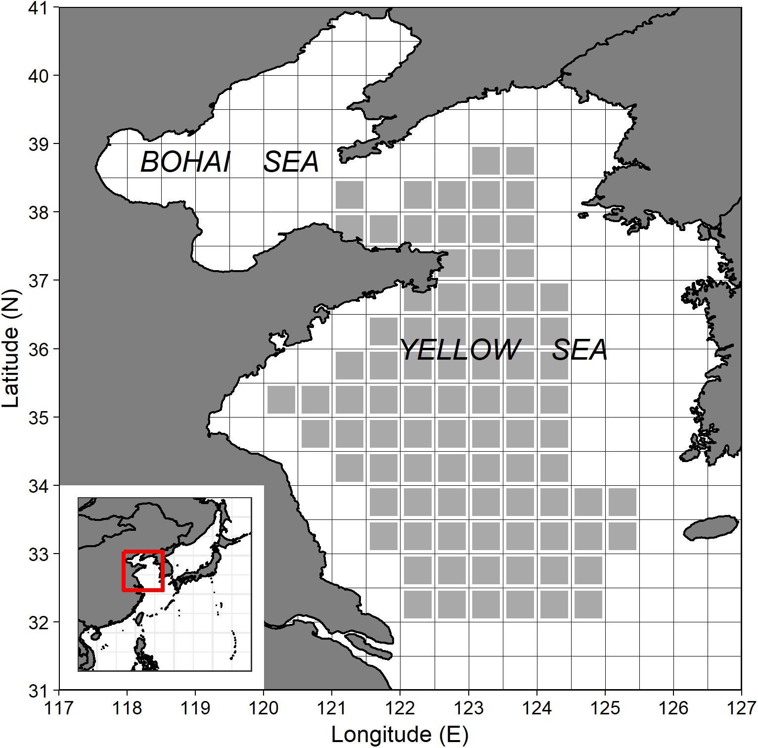
Figure 1. Map of Yellow Sea and bottom trawl survey stations (gray squares) during autumn from 2000 to 2018.

Scientific Survey Data

Scientific survey data were obtained from bottom trawl surveys conducted by the Yellow Sea Fisheries Research Institute (YSFRI), Chinese Academy of Fishery Sciences (CAFS) in autumn (October) from 2000 to 2018 (i.e., 2000, 2009, 2014, 2017, and 2018). Sampling stations were fixed inter-annually by a 0.5 × 0.5 grid (Figure 1). The same research vessel R/V “Beidou,” gear type (bottom trawl), and sampling protocol were used to ensure consistency over time. The trawl net had a cod-end mesh size of 2.4 cm, a headline height of 6.1–8.3 m, and a span of 25 m between its wings (Wu et al., 2020). The average trawl speed was 3.0 knots, and all tows were standardized to 1 h duration for each species at each station (Tanaka and Chen, 2016). A total of 392 valid tows (112 tows in 2000, 46 tows in 2009, 80 tows in 2014, 78 tows in 2017, and 76 tows in 2018) were included in the present study. The fishery-independent survey data included location (latitude and longitude) and number of individuals of each species. Each tow was assigned to a specific grid cell according to the survey location. The standardized number of individuals at each site for each species was used as AI. Zeros of AI were also used in this study because they were valid tows without catch for some species.

where AI_ijk is the standardized AI of species i at grid cell j in year k, Count_ijk is the sum number of individuals of species i across all tows assigned to grid cell j in year k, and Time_ijk is the sum tow duration (minutes) of species i across all tows assigned to grid cell j in year k.

Considering the abundance of each cephalopod species and the feasibility of model development, the top six species based on the number of individuals were selected in the present study. The data of 2000, 2009, 2014, and 2017 were used for HSI estimation, and those of 2018 were used for model prediction.

In the YS, T. pacificus, L. beka, and L. japonica are three dominant squids. However, the morphology of L. beka and L. japonica are too similar to distinguish, even for highly experienced fishers and fisheries experts. Therefore, L. beka and L. japonica were considered as one group named as Loliolus spp. while conducting surveys. Similarly, Euprymna morsei and Euprymna berryi were considered as one group named as Euprymna spp. for the same reason.

Fishing Intensity Data

Fishing intensity data for all species collectively from 2012 to 2016 (the only digital data available), including latitude, longitude, country of flag, fishing hours, gear type and date, were obtained from https://globalfishingwatch.org. Fishing hours were used as an index of fishing intensity. We filtered Chinese and Korean fishing vessels of all gear types operating in the YS, and the selected data were gridded to 0.25 × 0.25 then summarized annually for further analysis. Prior to mapping and statistical analysis, filtered effort data were converted to a log₁₀ scale after 1 was added to each effort (fishing hours) observation to account for zero values (Howell and Kobayashi, 2006; Mugo et al., 2010; Xue et al., 2017). Latitude was considered as categorical (each level of 1 degree), and the sampling design was unbalanced.

In order to determine if the total fishing hours showed a latitudinal shift with time, a two-way ANOVA test for unbalanced data was performed with effort (fishing hours) as the dependent variable and year (2012–2016), latitude (32°–40°) and country (China and Korea) as categorical explanatory variables. The Chinese fleet accounted for 99% of the total effort across the two nations. To examine all the effects, we included year × country, latitude × country interaction terms as well as year × latitude as the main interaction of interest (Table 1). The three-way interaction year × latitude × country was excluded because the number of observations (n = 90) was too small (df = 0). After testing for heteroscedasticity to ensure the data approximated a normal distribution, the power of the test was checked to confirm that replication was sufficient to detect a relatively small effect size (<10%) as described by Cohen (1988). The centroid of the spatial distribution of fishing effort was also calculated in each year for the same reason (i.e., to examine if fishing hours showed a latitudinal shift with time).

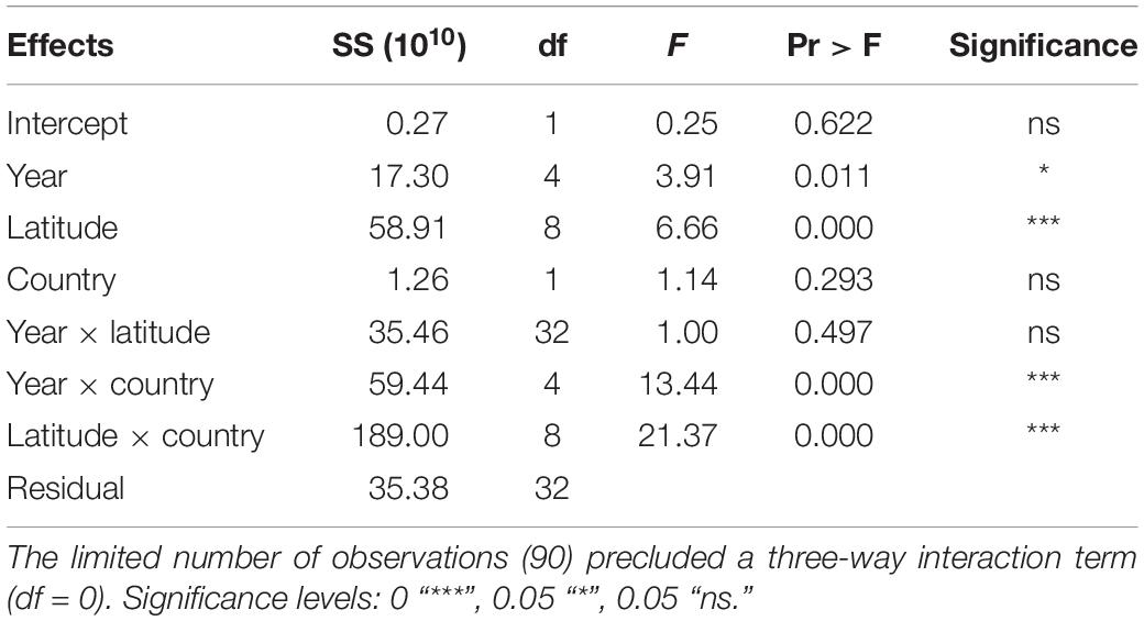
Table 1. Two-way ANOVA (Type III tests) of the main effects of year, latitude and country, and their two-way interactions on the effort (number of fishing hours) observed in the Yellow Sea during 2012–2016.

where G is the centroid (sometimes referred to as center of gravity) of fishing hours in each year, E_i is the total fishing hours at latitude category i of each year, and LAT is the mean latitude of latitude category i.

Fishing intensity data did not correspond with all years among the survey data (2000, 2009, 2014, 2017, and 2018), so fishing intensity was not integrated into the HSI development. Therefore, there was no need to attempt to align the spatial resolution of fishing intensity data with those of survey data and oceanographic data used in the HSI development. In order to see if the fishing intensity was directly influencing the spatiotemporal distribution of cephalopods, we mapped and compared the spatial distribution of fishing hours among years (Figures 2, 3).

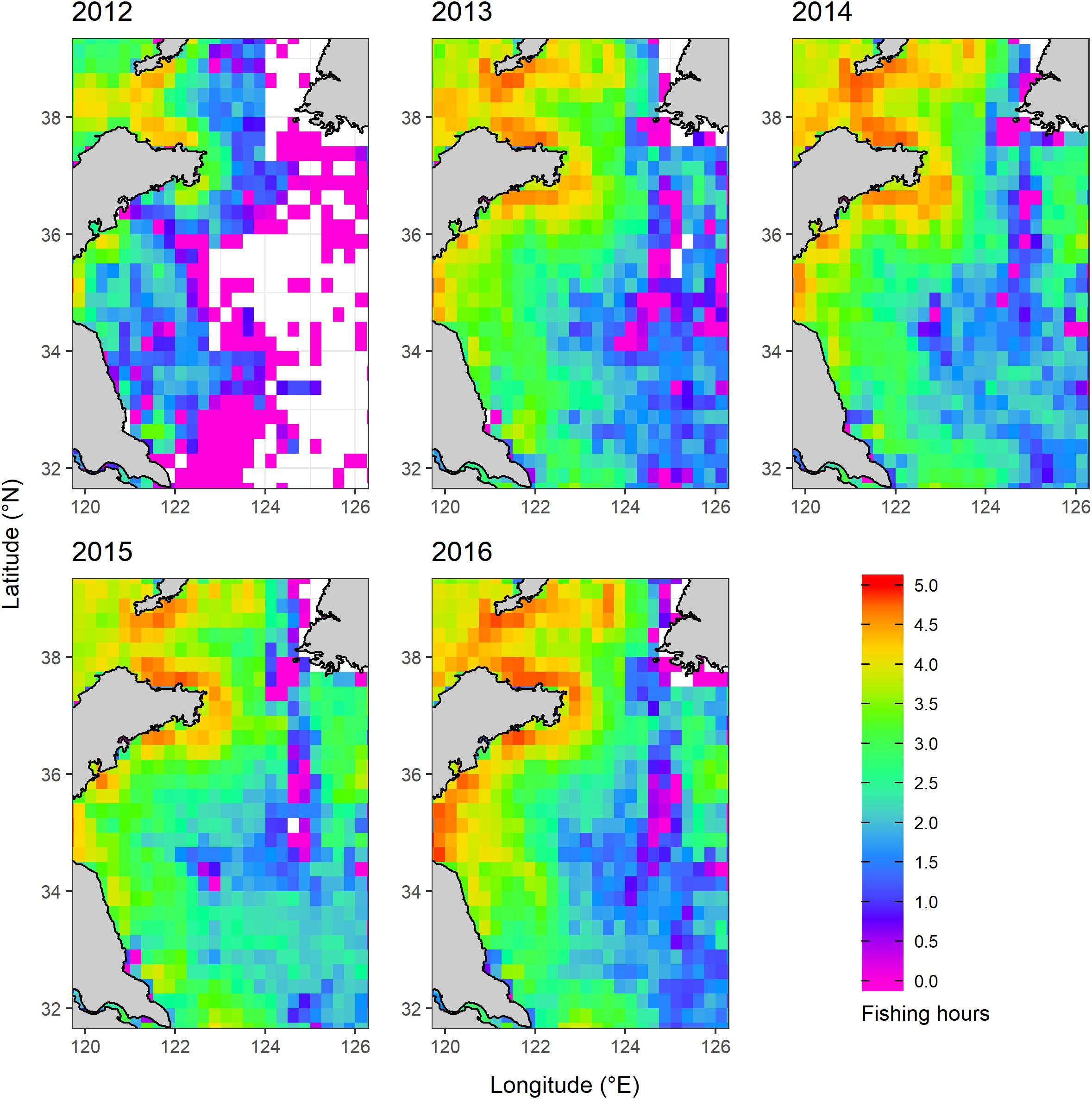
Figure 2. Spatial and temporal distribution of fishing intensity (represented by log transformed fishing hours) in the Yellow Sea.

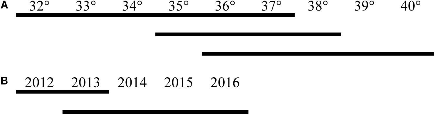
Figure 3. Tukey’s pairwise multiple comparisons (α = 0.05) illustrating consecutive latitudes (A) and years (B) for which contiguous lines indicate non-significant differences in fishing effort.

Oceanographic Variables

Oceanographic variables, including SST, SSHA, and CHLA, were initially selected based on existing knowledge about their vital impact on the distribution and abundance of cephalopods (Puerta et al., 2014; Keller et al., 2016; Yu et al., 2016a, b). Oceanographic data for October of 2000, 2009, 2014, 2017, and 2018 were obtained from a remote sensing database. Monthly SST (0.04 × 0.04 resolution) and CHLA (0.1 × 0.1 resolution for data in 2000 and 0.04 × 0.04 resolution for data in other years) data were from https://oceanwatch.pifsc.noaa.gov/. Monthly SSHA (0.17 × 0.17 resolution) data were from http://podaac-opendap.jpl.nasa.gov/. All the oceanographic variables were gridded to 0.5 × 0.5 for each October to match the spatial resolution of survey data prior to further analysis.

Habitat Suitability Index Development and Validation

SST, SSHA, and CHLA were selected as potentially vital oceanographic variables for the HSI, under an initial assumption that they were independent and had a strong influence on suitable habitat distribution. We assumed that the AI obtained from surveys reflected the natural distribution of cephalopods. To test for independence, we computed the correlation matrix for the three variables; SSHA was negatively correlated with SST (p < 0.01) and positively correlated with CHLA (p < 0.05), but there was no significant correlation between SST and CHLA (Figure 4). Although the coefficients were relatively low, at −0.16 for SSHA vs. SST and 0.13 for SSHA vs. CHLA, we dropped SSHA from the models.

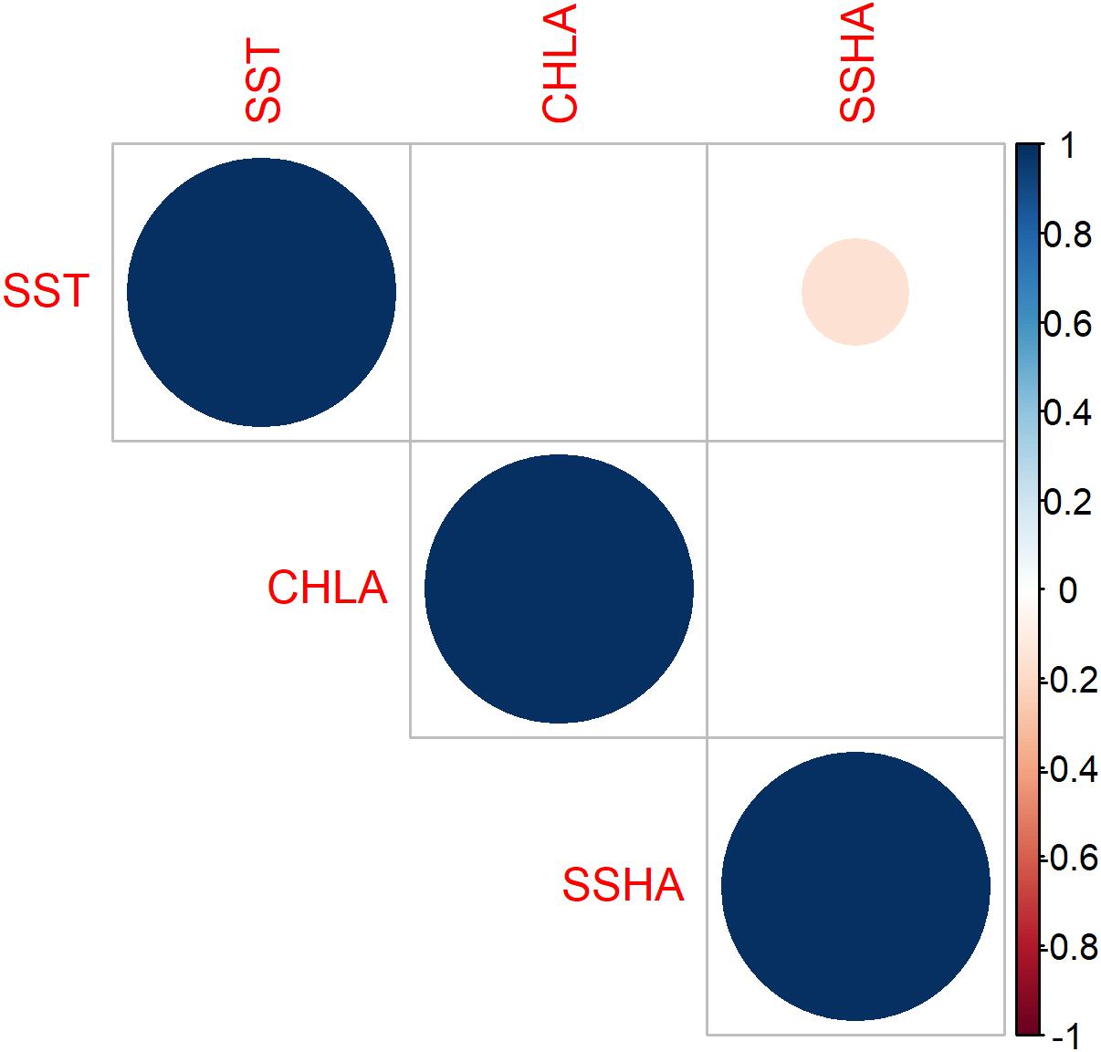
Figure 4. Cross-correlation plot of sea surface temperature (SST), sea surface height anomaly (SSHA), and chlorophyll-a concentration (CHLA) showing significant relationships (α = 0.05). Size of dots indicates strength of correlation and blanks where no correlation was detected.

For model development, we first built the suitability index (SI) using a smoothing cubic spline regression method in the generalized additive model (GAM) (from the “mgcv” package in R; Wood, 2017) to express the relationships between each of the two oceanographic explanatory variables (SST and CHLA) individually with the AI (response variable) as follows:

The GAM statements specified a negative binomial distribution with a log link function. The negative binomial distribution was selected to account for the over-dispersion from a preponderance of observations with low counts and zeros among the species abundance data. Only those models with significant effects were used, and where both variables were significant, then the one with the lowest p-value was selected except if one of the variables explained much more of the deviance than the other.

The SI has continuous values ranging from 0 (poor habitat) to 1 (optimal habitat). The SI for each species and each oceanographic variable was calculated based on the following equation (Tian et al., 2009; Chang et al., 2013; Xue et al., 2017):

where SI is the suitability index of each species at each grid cell, $\widehat{y}$ is the estimated value of AI using regression method, and ${\widehat{y}}_{max}$ and ${\widehat{y}}_{min}$ are the maximum and minimum values of estimated AI. SI values higher than 0.6 were regarded as within the optimal range, and the corresponding oceanographic variables were regarded as being within an optimal environmental range (Tian et al., 2009; Chang et al., 2013).

SI values obtained from the additive models were subsequently incorporated into the HSI formula using two different estimation methods, the geometric and the arithmetic means as follows (Chen et al., 2009; Tian et al., 2009; Chang et al., 2013):

where SI_i is the suitability index value based on the oceanographic variable i, and n is the number of oceanographic variables considered.

A cross-validation method was used to evaluate the performance of the HSI. Indices were developed independently for each species by modeling 80% of the data selected randomly from 2000–2017 as training data and the rest from that period as testing data to assess the performance of the index in each instance (Zuur et al., 2007; Tanaka and Chen, 2015). Linear regression analysis was used to compare the estimated HSI values between training data and testing data, whose results including the regression intercept, slope, R² value, and the Akaike information criterion (AIC) score were used to evaluate the fit of the HSI in each instance. The closer the intercept was to 0, the slope to 1, the higher the R² value, and the lower the AIC value, the better the model was considered to have fitted the data. One hundred cross-validation runs were conducted using random selection for each run to obtain 100 sets of regression parameters. This validation process was conducted to identify the model which performed best for each of the AMM- and GMM-based HSI (Tanaka and Chen, 2015).

We then applied these AMM- and GMM-based models developed with the 2000–2017 data to predict SI and then calculate HSI using the environmental data (based on CHLA or SST for each species as appropriate) for 2018. We then established a new model using the 2018 data, and estimated SI and then calculated HSI using the environmental data for 2018. This process produced a set of estimated and predicted HSI for each species in each grid cell surveyed in 2018. To determine whether the AMM- or GMM-based performed best for each species, we calculated the mean square error of prediction (MSEP) for each of these two model types for each species, i.e.,

where HSI_E is the estimated HSI of 2018 derived from the relationship of 2018, and HSI_P is the predicted HSI of 2018 derived from the relationship of 2000–2017. The lower the value of MSEP for a model, the better is its performance (Björkwall et al., 2011).

The spatial distribution of AI in October of 2018 was then overlaid on the predicted AMM- and GMM-based HSI maps of the same year to provide a visual comparison. AI data from 2000 to 2017 were rescaled (divided by the maximum abundance of each species among years) to plot AI distribution to see if there are different distribution patterns of each species among years.

Results

Interannual Variation of the Fishing Intensity

Based on the spatial and temporal fishing density data from Global Fishing Watch, the lowest fishing intensity was in 2012 while the highest was in 2016. The fishing intensity did not increase gradually with years (except 2012). The inshore area of China had the highest fishing intensity among all years, while the central YS had the lowest fishing intensity (Figure 2). The inshore area of China in the northern YS had the highest fishing intensity and gradually decreased to the south among all years.

The total fishing hours showed that fishing intensity in 2012 had the lowest values (gray dots in Figure 5). Generally, the most intense fishing was concentrated in the latitude range of 38–39°N and gradually decreased from north to south. The fishing intensity of 39–40°N was, however, similar to those of 35–36°N and 36–37°N (Figure 5). Linear regression of the centroid of fishing hours showed that the slope was weakly significant (p > 0.01, black dots in Figure 5). Two-way ANOVA testing showed that although the full model and year × latitude were non-significant (P > 0.1), year × country, and latitude × country were highly significant (p < 0.001) (Table 1). This implies that latitudinal differences in fishing hours remained consistent over time (Figure 5). Tukey’s pairwise post hoc comparisons showed that the temporal increase in effort was confined to the annual interval at the start of the series, i.e., 2012–2013 when average fishing hours increased by 34% (Figure 3).

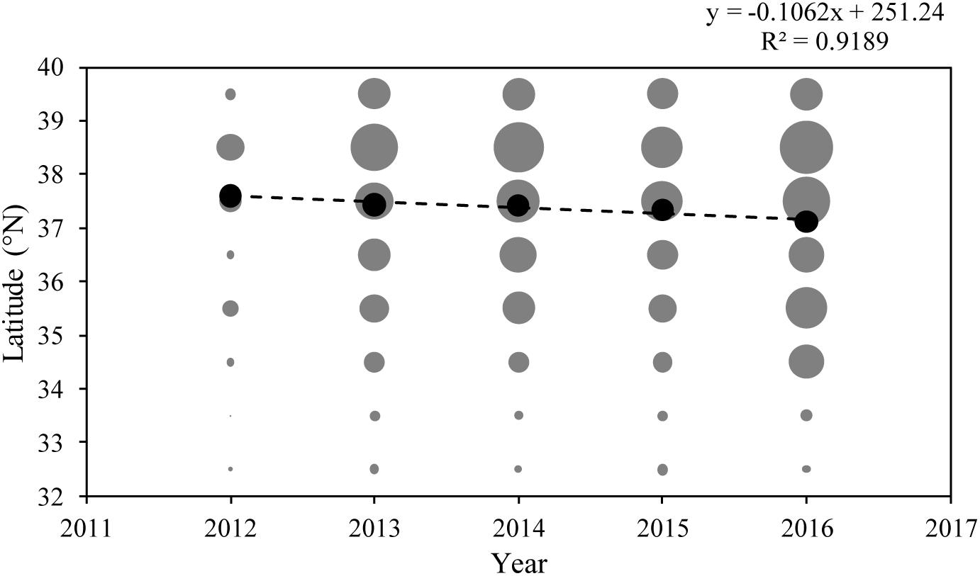
Figure 5. Inter-annual and latitudinal trends of fishing intensity (represented by sum of log₁₀ transformed fishing hours) in the Yellow Sea. Gray dots represent total fishing hours of each latitudinal category in each year, black dots represent the centroid of total fishing hours in each year, and linear regression was given based on gravity center.

Interannual Variation of the Oceanographic Variables

The oceanographic data acquired during October of 2000, 2009, 2014, 2017, and 2018 were selected for analysis in accordance with the survey period. The oceanographic variables changed spatially in the same year, and there were also interannual variations for each of them (Figure 6). SST decreased with increasing latitude and decreased sharply around 34°N. It had the highest values at 32–33°N in 2000 and early October of 2009, whereas the lowest SST occurred at about 38°N. Across the longitudinal range, SST was lowest at approximately 121°E in 2009, 2014, and 2017, 123.5°E in 2014, and 126°E in 2017 and 2018. In accordance with SST, CHLA showed significant change at 34°N in all years. The CHLA had lower values between 32°N and 34°N in all years except 2000 and 2018 when it was at 36°N, whereas higher values were evident at 38°N. Higher CHLA values longitudinally were located between 121.5°N and 126°E in 2009 and 126°E during 2009–2017, whereas lower CHLA values occurred between 122.5°N and 124°E in 2000, 2014, 2017, and 2018.

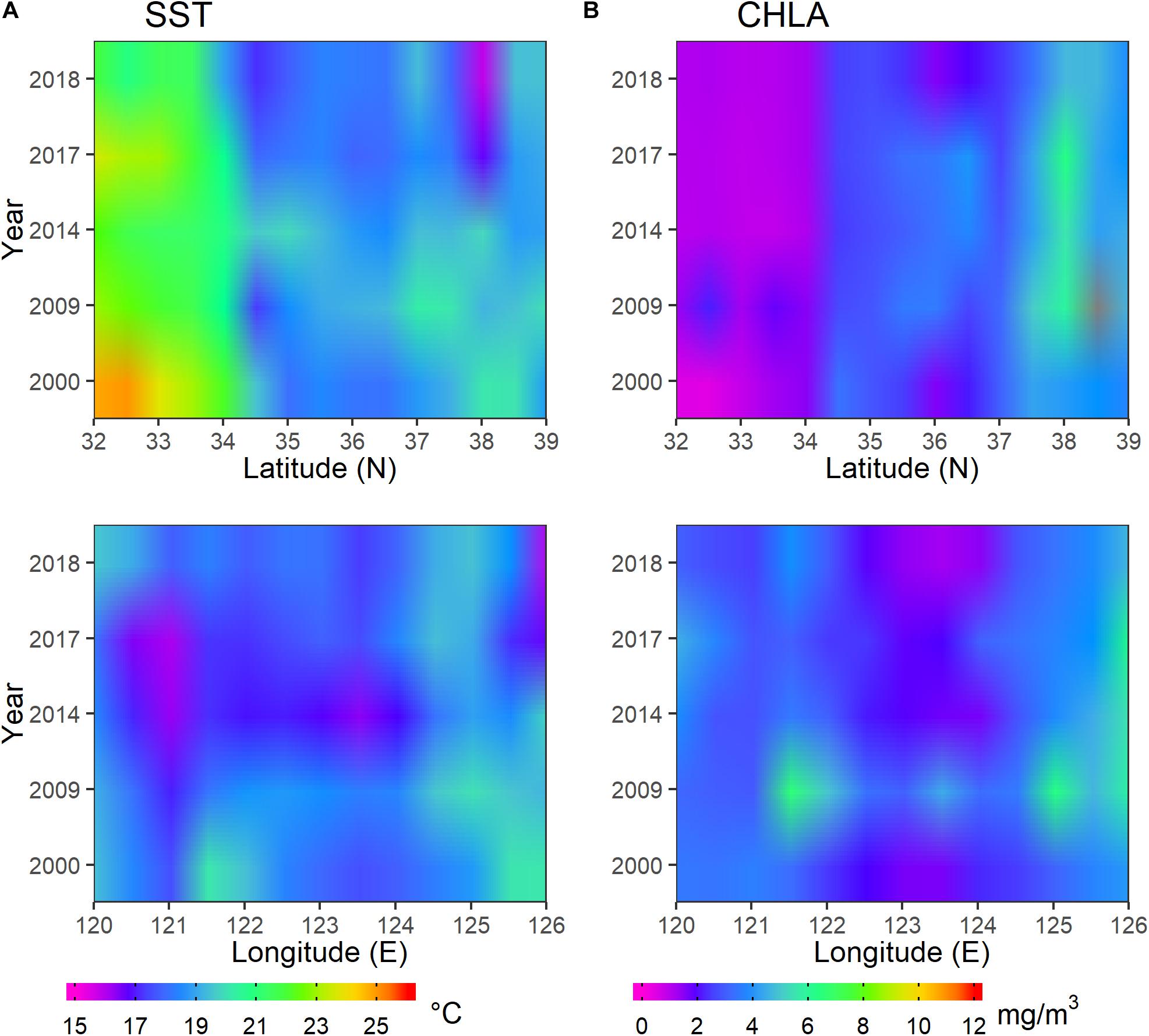
Figure 6. Spatiotemporal distribution of monthly oceanographic variables in October of 2000, 2009, 2014, 2017, and 2018 for (A) sea surface temperature (SST) and (B) chlorophyll-a concentration (CHLA).

Relationships Between Abundance Index and Oceanographic Variables

The regression analyses indicated that the better performing variable differed among species (Table 2). For T. pacificus, Loliolus spp., O. variabilis, and O. ocellatus, the SI model for CHLA was statistically significant (p < 0.05), explaining the most deviance and had the smallest AIC value, making it the preferred oceanographic variable to establish SIs. For S. birostrata and Euprymna spp., the abundance for SST explained the most deviance, had the smallest AIC value, and was statistically significant (p < 0.05), although the p-values were marginal for S. birostrata.

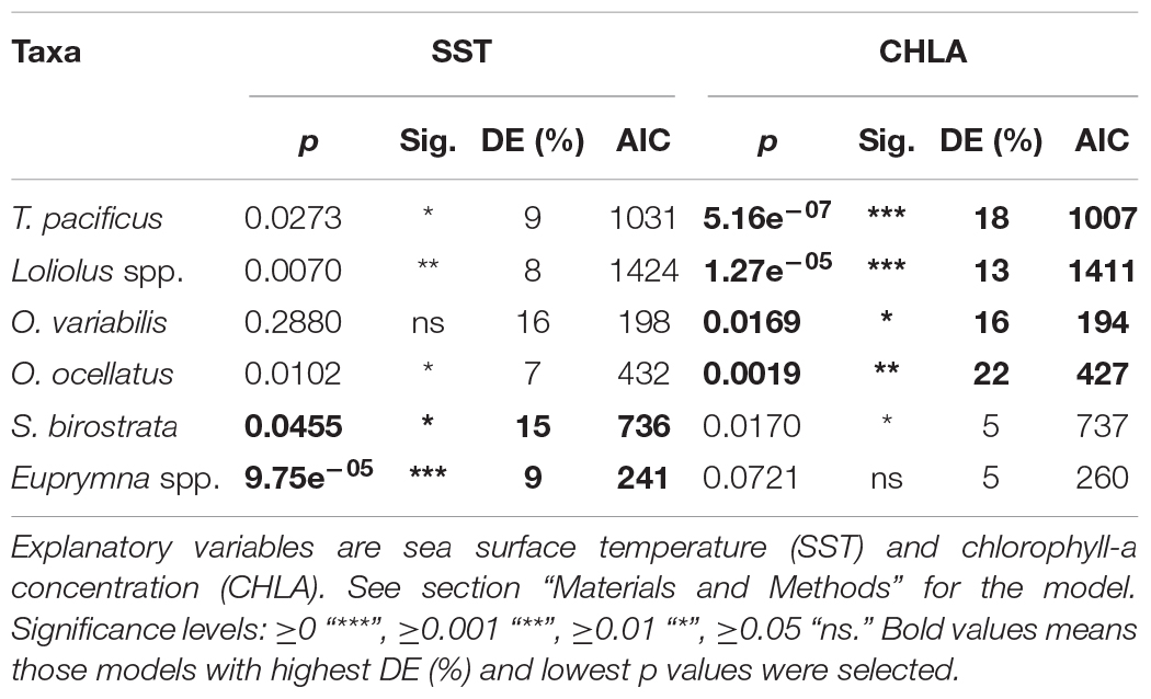
Table 2. Generalized additive model (GAM) outputs of the abundance of the six cephalopod taxa.

According to the fitted SI models for SST, the optimal SST ranges were 16.0°C–17.8°C (and 20.2°C–20.9°C, 22.9°C–23.2°C), 18.6°C–20.9°C, 18.6°C–20.6°C (and 21.1°C–22.9°C), 16.3°C–19.6°C, 20.1°C–21.6°C, and 16.0°C–17.9°C (and 20.4°C–20.9°C, 22.9°C–23.2°C) for T. pacificus, Loliolus spp., O. variabilis, O. ocellatus, S. birostrata, and Euprymna spp., respectively (Figure 7).

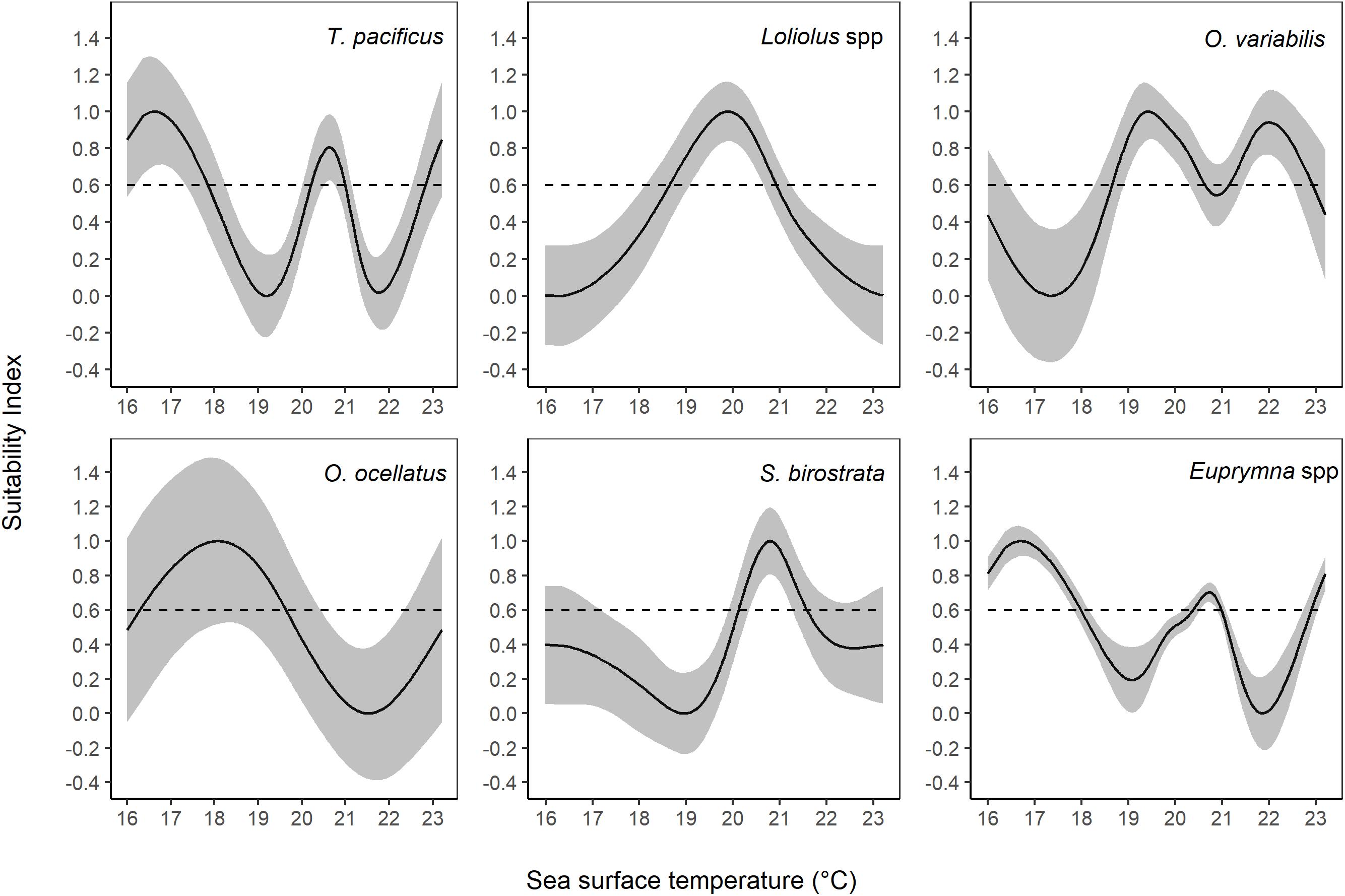
Figure 7. Suitability index (SI) for sea surface temperature (SST) based on the smoothing spline regression method.

The optimal CHLA ranges were 0.67–2.44 mg/m³, 2.30–3.76 mg/m³, 1.82–3.58 mg/m³, 2.92–4.64 mg/m³, 0.48–1.65 mg/m³ (and 4.22–4.64 mg/m³), and 0.48–2.24 mg/m³ for T. pacificus, Loliolus spp., O. variabilis, O. ocellatus, S. birostrata, and Euprymna spp., respectively (Figure 8).

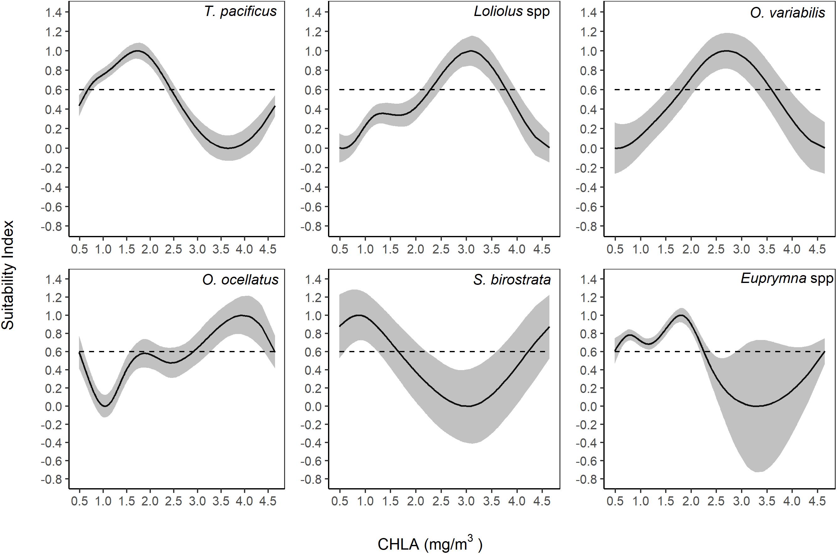
Figure 8. Suitability index for chlorophyll-a concentration (CHLA) based on the smoothing spline regression method.

Interestingly, some relationships had more than one peak of SI over 0.6, i.e., SST for T. pacificus, O. ocellatus, and Euprymna spp., and CHLA for S. birostrata.

Habitat Suitability Index Comparison, Selection, and Validation

For each species, the cross-validation regression between predicted and estimated HSI showed that the intercepts (α) of the GMMs were closer to 0 compared with the AMMs (except for Euprymna spp.) (Table 3). In contrast, the slopes of the AMMs were closer to 1 compared to the GMMs (except for O. variabilis and Euprymna spp.). For the R², those of the AMMs were higher than those of GMMs (except for O. variabilis, S. birostrata). When compared with an ideal model without prediction bias (α = 0, β = 1, and R² = 1), the AMM of Loliolus spp. had the best performance (α = 0.20, β = 0.59, and R² = 0.57) among all species. For each species, both MSEP and SD of predicted HSI values based on AMM was lower than that based on GMM (Table 4).

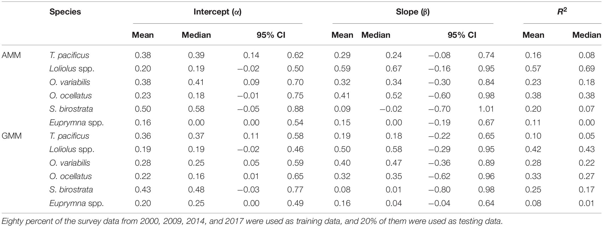
Table 3. Summary of linear regression analyses between the predicted and estimated habitat suitability index (HSI) values for the arithmetic mean method (AMM) and the geometric mean method (GMM) from 100 cross-validation runs.

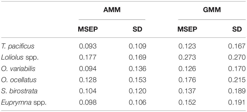
Table 4. Comparison of the mean square errors of prediction (MSEP) and their standard deviations (SDs) for arithmetic mean method (AMM)- and geometric mean method (GMM)-based habitat suitability index (HSI) for each cephalopod species derived from 2018 data.

Distribution Pattern Based on Abundance Index and Habitat Suitability Index

According to the map of predicted HSI overlaid with AI of 2018 and AI from 2000 to 2017 (Figures 9, 10), distribution patterns differed among species. Todarodes pacificus was distributed in deeper water of the YS, and the model prediction also showed high density in deep water. Loliolus spp. and O. ocellatus showed higher abundances and HSI values in the coastal area. O. variabilis was distributed in deeper water of the YS, while the model prediction showed high density in coastal water. There were deep-water distribution tendencies for S. birostrata and Euprymna spp. in the predicted and survey results. The AI distribution of each species showed different patterns between decades (i.e., 2000s vs. 2010s) (Figure 10).

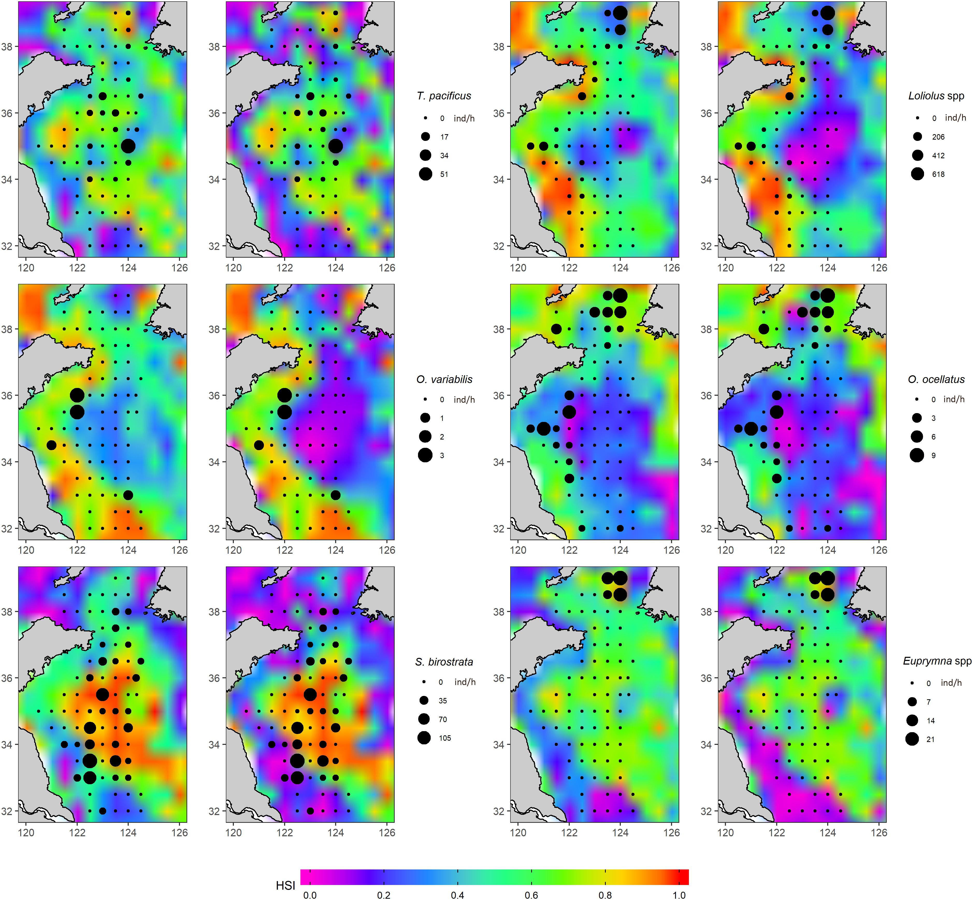
Figure 9. Habitat suitability index (HSI) map of cephalopods predicted based on the oceanographic data (sea surface temperature and chlorophyll-a concentration) in 2018 using an arithmetic mean model (AMM) and a geometric mean model (GMM) developed with data from 2000 to 2017. A cephalopod abundance index (AI) distribution from 2018 was overlaid on the HSI map. The left panel of each species represents its respective AMM, and the right panel of each species represents its respective GMM.

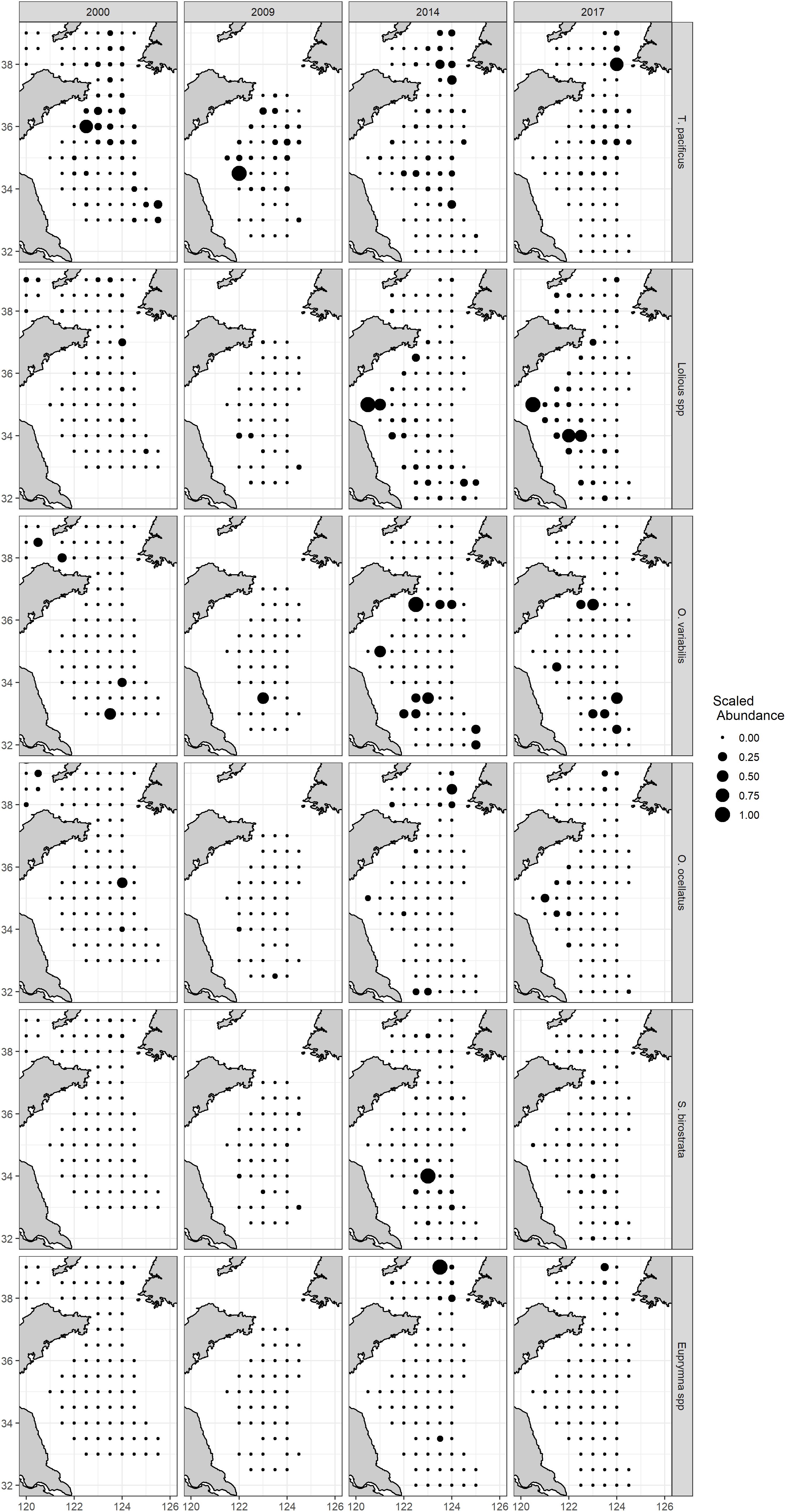
Figure 10. Scaled spatial distribution of abundance index (AI) of different species per year (2000–2017).

Discussion

The absence of a significant interaction effect between year and latitude, despite the high power of the analysis of variance, is consistent with changes in spatial distribution patterns of cephalopod abundance arising from the consequences of changing environmental conditions rather than directly from geographic changes in patterns of fishing intensity. This was not unexpected as total fishing hours in the north of the YS were consistently higher than for the south throughout the study period (Figure 5). Although there was a weak southward trend in the centroid of fishing effort over the study period, the displacement was small at about 0.5° in latitude so would have only made a slight contribution to northerly increases in species population abundance. The latitude range of 37°N–39°N had the most intense total fishing hours in all years, which could result in a higher fishery exploitation rate in this area. In this case, if the abundance of high trophic level species reduced because of overexploitation (Rosa et al., 2019), cephalopod abundance of this overexploited fishing ground could then increase due to their pronounced phenotypic plasticity and a reduction in their predators (Doubleday et al., 2016; Liscovitch-Brauer et al., 2017). HSI modeling can provide robust and highly predictive habitat quality estimates for marine organisms (especially those targeted by fisheries) using environmental variables (Yu et al., 2015). In the present study, we integrated AI, SST, and CHLA into two empirical methods to establish HSI and to interpret the relationships between the spatial distributions of cephalopods and environmental variables using abundance data acquired from scientific surveys in the YS and environmental data derived from satellites. The survey data from YSFRI’s annual autumn stock monitoring program used in the present study reflect the spatial distribution of marine species much better in comparison with fishery-dependent data. Fishers tend to mostly fish in small areas yielding large catches associated with high-quality habitat (Yu et al., 2018). Fishers are unwilling to fish those areas with low fish abundance, due to their lower profitability, which means fisheries usually operate within a highly concentrated area. Therefore, it is impractical to attempt to establish a species distribution map over a wide geographic range solely based on fishery-dependent data. In contrast, scientific surveys conducted independently of fishing in the YS are designed in an organized grid of fixed monitoring stations that can more reliably reflect the distribution pattern in the entire study area (Jin et al., 2005). Hence, fishery-independent scientific survey data from well-designed motoring programs are much more powerful than fishery-dependent data in terms of modeling spatial distributions. In the context of YS with a mean water depth around 40 m and maximum depth around 150 m, the bottom trawl survey that we used emerged as a very good method for investigating fisheries resources in this area.

Oceanographic variables can be used as predictors of the physiological suitability, food availability, and oceanic physical conditions of habitats (Mohri, 1999; Chen et al., 2010). Each cephalopod species or group investigated in the present study showed unique environmental preferences, which can account for their different spatial distributions. SST, SSHA, and CHLA were considered as proxy oceanographic variables that can identify the most suitable habitat for specific cephalopod groups (Arkhipkin et al., 2015). However, SSHA was correlated with SST and CHLA, and SSHA showed a non-significant linear relationship with the abundance of each species except for S. birostrata. Therefore, we only used SST and CHLA for HSI modeling. After establishing the relationship between the AI of each species and the two oceanographic variables, we found that CHLA was the most important oceanographic variable for squid and octopus, whereas SST was the most important for bobtail squid. This may relate to differences in their habitat requirements after reaching a catchable size. Octopus and bobtail squid are benthic species that spend their juvenile and adult life history stages at the bottom near the seabed; T. pacificus is an oceanic species that usually inhabits the middle of YS; Loliolus spp. is usually located near the bottom during daytime and near the surface at night (Dong, 1988; Jereb and Roper, 2006, 2010). Because of the small size of Loliolus spp., hydrological currents have a strong influence on their abundance and distribution while they are near the surface in the water column. Survey data from this study showed that Euprymna spp. usually inhabits locations north of 37°N, making them very sensitive to temperature, which explains why they exhibited a very strong relationship with SST (Table 2 and Figure 7). T. pacificus and Loliolus spp. exhibit diel migration and will swim up to the surface during the night, which explains their strong relationship with CHLA. Habitat preference of other species with strong diel migration, such as swordfish (Xiphias gladius), jumbo flying squid (Dosidicus gigas), neon flying squid (Ommastrephes bartramii), chub mackerel (Scomber japonicus), and jack mackerel (Trachurus murphyi) is also heavily influenced by CHLA (Chang et al., 2013; Yu et al., 2015, 2018, 2019; Li et al., 2016). O. variabilis and O. ocellatus, were weakly or not associated with SST, reflecting their benthic lifestyle (Dong, 1988; Jin et al., 2005). Caution is warranted, nevertheless, when interpreting the observed relationships between AI and oceanographic variables because some showed inconsistent trends (Figures 7, 8). We acknowledge that these results were relative to the models we tested and that our results are not necessarily the best solutions for the relationships between the AI and oceanographic variables more generally. The reasons for variation in trends may be because (1) the data we used only included 1 month (October) for all years which may have excessively narrowed the period during which the range of a specific oceanographic variable would be expected to be suitable for some species; and (2) some species were located in areas with distinctly unique environments which create the potential for more than one peak of certain oceanographic variables: take the abundance distribution of 2018 for example (Figure 9), in which Loliolus spp. had three distinctly high abundance areas, and both O. variabilis and O. ocellatus had at least two distinctly high abundance areas.

In the present study, consistent with findings from other studies, suitable habitats were those with SI values above 0.6 (Chang et al., 2013; Yu et al., 2016a). Suitable habitats for T. pacificus, O. ocellatus, and Euprymna spp. seemed to be concentrated in areas with relatively low SST, while other species were concentrated in areas with high SST. T. pacificus exhibits long-distance migration in its life history and only stays in the YS for feeding from May to December, after which it then migrates back to the East China Sea (ECS) for spawning. During the feeding period in the YS, a branch of T. pacificus migrates to the northern YS around 37°N and remains in the mass of cold-water in that area during summer and autumn (Jin et al., 2005). Since the surveys for the present study were conducted during October, it is reasonable to infer that the suitable habitat for T. pacificus is distributed in areas of low SST. The HSI map also showed that T. pacificus prefers offshore areas with deeper water depths (Figure 9). Yu et al. (2015) found a similar pattern for O. bartramii in the Northwest Pacific. T. pacificus spent its summer and early fall in the northern region of the YS for feeding, and its suitable temperature range for high habitat quality was 16°C–17°C in October. O. ocellatus is a classic cold-water species, which makes sense in that it had a low SST for its suitable habitat. For Euprymna spp., we found that it was usually distributed in the northern YS in a small area in October (not shown in this paper), which was consistent with the HSI prediction map that showed high HSI values for the northern YS. Dong (1988) identified E. morsei and E. berryi in different China Seas and inferred that Zhoushan Islands was the geographical boundary separating these two species, i.e., E. morsei lived in the north while E. berryi lives in the south, based on existing inventories of specimens collected during scientific surveys, which means E. morsei lived in relative cold water compared to E. berryi.

There are several alternative methods which can be used for establishing HSI, such as the continued product model, the minimum model, the maximum model, generalized linear model, and GAM (Van der Lee et al., 2006; Chen et al., 2008; Guo and Chen, 2009; Chang et al., 2013). However, most of these methods would either underestimate or overestimate the HSI values (Yu et al., 2018). Instead, we used the AMM- and GMM-based HSI to make better predictions of the suitable habitat distribution of cephalopods.

The cross-validation results (Table 3) and MSEP of HSI (Table 4) showed that the HSI based on AMM outperformed the GMM, which is consistent with several previous papers that have reported on different species (Chen et al., 2009; Tian et al., 2009; Li et al., 2014; Tanaka and Chen, 2015; Yu et al., 2015, 2016b; Silva et al., 2016; Yen et al., 2017). The two models we compared have different assumptions: the AMM assumes that variables can compensate for each other dependently to explain the ideal habitat conditions, whereas the GMM has compensatory effects that give less importance to extreme values (Chang et al., 2013). Both models assume that the explanatory variables have equal impacts on each species’ habitat distribution (Vayghan et al., 2013). This will not be the case in reality because oceanographic variables have different impacts on spatiotemporal distribution, which could substantially influence the predictive performance of the HSI (Gong et al., 2012). To deal with this issue in future studies, different weights should be given to the oceanographic variables to improve the predictive performance of the HSI. Before weighting oceanographic variables, a full model that includes all oceanographic variables should be tested to determine the importance of each variable. As can be seen from Figure 2, there are no groundfish areas that are designated closed areas in our study region, which means that we cannot distinguish between fished and pristine areas to establish if the HSI returns different values between them. We do, however, have a summer fishing moratorium from May 1 to August 31 in the YS, which means we can ascertain if HSI returns different values within fishing and non-fishing periods. In addition, given sufficient concurrence among years of fishing effort data and annual surveys, comparisons between intensively fished areas with those that are seldom or less intensively fished could be made, and seasonal effects of fishing intensity identified from intra-annual spatial patterns of fishing effort, by including fishing intensity in the HSI.

Loliolus spp., T. pacificus, and S. birostrata were the most abundant cephalopod species in the taxa composition of samples taken during the autumn scientific surveys. Except for S. birostrata, five of the cephalopod species were predominantly distributed north of 34°N, which according to the 2018 spatial distribution map may be related to SST and CHLA (dots in Figure 9). We found that both SST and CHLA changed significantly around 34°N during October for each year of the study period (Figure 6), which may indicate that this latitude represents a natural barrier for those species. In contrast, S. birostrata had a wider spatial distribution range, which can be explained by its different life strategy to that of other neritic cephalopods. Although S. birostrata is defined as a neritic cephalopod, records show that it can live in deeper water (Dong, 1988). During a survey in the 1980s, the R/V “Jingxing” from the Institute of Oceanology, Chinese Academy of Sciences, captured an adult individual of S. birostrata at a depth of 1,100 m in the South China Sea (SCS), and the R/V “Albatross” from the United States captured S. birostrata at depths of over 200 m near Japanese islands on several occasions (Dong, 1988). The spatial distribution based on our HSI and survey in 2018 suggested that T. pacificus, S. birostrata, and Euprymna spp. prefer to live in the deep water of the YS, while Loliolus spp., O. variabilis, and O. ocellatus prefer to live near the coast. Cephalopods now prefer to live in the north of the YS rather than the south compared with previous observations during the last two decades (Figures 9, 10). It is plausible that this represents a poleward displacement as preferred habitat and environmental conditions shift northward due to impacts such as climate change. Surveys conducted by Russian and Norwegian researchers have demonstrated that cephalopod composition and distribution ranges in the Arctic have changed in association with the effects of climate-induced environmental shifts during the last two decades (Golikov et al., 2013). However, each species had its own response to a changing environment. Loliolus spp. showed a northward distribution trend, while T. pacificus showed a northward distribution trend and returned back to the south in 2018; this may relate to high CHLA in 2014 and 2017 and low CHLA in 2018 around 38°N. The distribution of O. variabilis showed a restriction of its distribution, which is caused by cold-water mass in the middle YS. O. ocellatus and S. birostrata of 2018 distributed in wider area in the south than those of previous years; this may relate to low SST of 2018 in the south. Euprymna spp. remained at northmost of the study area for most years because it belongs to cold-water species as discussed above (Figures 7, 9, 10). Although the AI distribution of each species showed different patterns between decades (Figure 10), the models (especially AMM-based HSI) still showed good performance by matching suitable habitats based on HSI with the survey data acquired during 2018.

In conclusion, we conducted a simple analysis of the spatiotemporal distribution of fishing intensity (represented by fishing hours) and used AMM- and GMM-based HSI to predict the spatial distribution of cephalopods in the YS. We found that latitudinal differences in fishing intensity remained largely consistent during the study period, but with a small southerly trend that would be unlikely to account for much larger northward shifts in species distributions. We also found that there was a dramatic change in SST and CHLA around 34°N, which may be affecting the spatial distribution of cephalopods. CHLA was the most important oceanographic variable influencing the distributions of squid and octopus, while SST was the most important variable for influencing change in bobtail squid distribution, which reflects differences in their life history traits. The AMM-based HSI performed better than the GMM-based HSI according to the MSEP. Survey data are expected to be more powerful than fishery-dependent data in terms of mapping the breadth of species distributions. In the autumnal month of October, T. pacificus and S. birostrata were mainly distributed in colder water found at greater depths in the YS, whereas Loliolus spp., O. ocellatus, and O. variabilis were mainly distributed in warmer inshore areas, and Euprymna spp. was distributed across a wide range of territory (both inshore and offshore). The models predicted that the distributions of oceanic and bobtail squid were comparable to those of octopuses and neritic squid, which may reflect generalized habitat selection in accordance with oceanographic variables. Since the relative impacts of different oceanographic variables on spatiotemporal distribution will be heterogeneous, further studies should assign different weights to each oceanographic variable in the HSI to provide more precise predictions about spatial distributions in response to environmental pressures such as those anticipated from global climate change. Future research should focus on extending this work to develop a more holistic regression incorporating all variables into a single model for cephalopod habitat suitability in the YS. A more in-depth study of the cephalopods we investigated and other congeneric species is needed to gain a better understanding of their spatial distributions and ecology.

Data Availability Statement

The fishing effort dataset analyzed for this study can be found on https://globalfishingwatch.org. The environmental datasets analyzed can be found on https://oceanwatch.pifsc.noaa.gov/ and http://podaac-opendap.jpl.nasa.gov/. The scientific fishery survey dataset analyzed is not publicly available. Requests to access these datasets should be directed to [Dr. XS/Yellow Sea Fisheries Research Institute, Chinese Academy of Fishery Sciences (shanxj@ysfri.ac.cn)].

Ethics Statement

Ethical review and approval was not required for the animal study because our research is related to fisheries, and our data were from scientific fishery surveys. No extra experiment was conducted.

Author Contributions

YJ, XJ, and XS conceived the study. XJ, XS, and QW collected the survey data. YJ and HG collected the fishing effort data, analyzed the data, and wrote the manuscript. All authors contributed to the article and approved the submitted version.

Funding

This study was supported by the National Natural Science Foundation of China (31872692), National Key R&D Program of China (2017YFE0104400), Taishan Scholar Project of Shandong Province, and Central Public-Interest Scientific Institution Basal Research Fund, CAFS (No. 2019GH16).

Conflict of Interest

The authors declare that the research was conducted in the absence of any commercial or financial relationships that could be construed as a potential conflict of interest.

Acknowledgments

We thank the colleagues from the Division of Fishery Resources and Ecosystem, Yellow Sea Fisheries Research Institute, Chinese Academy of Fishery Sciences, for measuring and sampling during the long-term surveys. We also thank Luoliang Xu, Zhou Fang, and Gang Li for their helpful R programming. Special thanks to Drs. Khageswor Giri and Lisha Guan for statistical advice and two reviewers for their valuable and constructive comments on the manuscript.

References

Adams, C. F., Alade, L. A., Legault, C. M., O’Brien, L., Palmer, M. C., Sosebee, K. A., et al. (2018). Relative importance of population size, fishing pressure and temperature on the spatial distribution of nine Northwest Atlantic groundfish stocks. PLoS One 13:e0196583. doi: 10.1371/journal.pone.0196583
Arkhipkin, A. I., Rodhouse, P. G., Pierce, G. J., Sauer, W., Sakai, M., Allcock, L., et al. (2015). World squid fisheries. Rev. Fish. Sci. Aquac. 23, 92–252. doi: 10.1080/23308249.2015.1026226
Bastardie, F., Nielsen, J. R., Ulrich, C., Egekvist, J., and Degel, H. (2010). Detailed mapping of fishing effort and landings by coupling fishing logbooks with satellite-recorded vessel geo-location. Fish. Res. 106, 41–53. doi: 10.1016/j.fishres.2010.06.016
Björkwall, S., Hössjer, O., Ohlsson, E., and Verrall, R. (2011). A generalized linear model with smoothing effects for claims reserving. Insur. Math. Econ. 49, 27–37. doi: 10.1016/j.insmatheco.2011.01.012
Chang, Y. J., Sun, C. L., Chen, Y., Yeh, S. Z., DiNardo, G., and Su, N. J. (2013). Modelling the impacts of environmental variation on the habitat suitability of swordfish, Xiphias gladius, in the equatorial Atlantic Ocean. ICES J. Mar. Sci. 70, 1000–1012. doi: 10.1093/icesjms/fss190
Chen, X. J., Feng, B., and Xu, L. X. (2008). A comparative study on habitat suitability index of bigeye tuna, Thunnus obesus in the Indian Ocean. J. Fish. Sci. China 15, 269–278. doi: 10.3321/j.issn:1005-8737.2008.02.011
Chen, X. J., Li, G., Feng, B., and Tian, S. Q. (2009). Habitat suitability index of Chub mackerel (Scomber japonicus) from July to September in the East China Sea. J. Oceanogr. 65, 93–102. doi: 10.1007/s10872-009-0009-9
Chen, X. J., Tian, S. Q., Chen, Y., and Liu, B. L. (2010). A modeling approach to identify optimal habitat and suitable fishing grounds for neon flying squid (Ommastrephes bartramii) in the Northwest Pacific Ocean. Fish. Bull. 108, 1–14.
Ciannelli, L., Fisher, J. A. D., Skern-Mauritzen, M., Hunsicker, M. E., Hidalgo, M., Frank, K. T., et al. (2013). Theory, consequences and evidence of eroding population spatial structure in harvested marine fishes: a review. Mar. Ecol. Prog. Ser. 480, 227–243. doi: 10.3354/meps10067
Cohen, J. (1988). Statistical Power Analysis for the Behavioral Sciences, 2nd Edn. New York, NY: Routledge, 567.
Doubleday, Z. A., Prowse, T. A., Arkhipkin, A., Pierce, G. J., Semmens, J., Steer, M., et al. (2016). Global proliferation of cephalopods. Curr. Biol. 26, R406–R407. doi: 10.1016/j.cub.2016.04.002
Du, T. F., Li, A., Dai, F. Q., Li, D., Liu, S. F., and Zhuang, Z. M. (2016). Survey and analysis of the autumnal cephalopod distribution in the Yellow Sea during 2006–2013. J. Fish. Sci. China. 23, 955–964. doi: 10.3724/SP.J.1118.2016.15381
Golikov, A. V., Sabirov, R. M., Lubin, P. A., and Jørgensen, L. L. (2013). Changes in distribution and range structure of Arctic cephalopods due to climatic changes of the last decades. Biodivers 14, 28–35. doi: 10.1080/14888386.2012.702301
Gong, C. X., Chen, X. J., Gao, F., and Chen, Y. (2012). Importance of weighting for multi-variable habitat suitability index model: a case study of winter-spring cohort of Ommastrephes bartramii in the Northwestern Pacific Ocean. J. Ocean. U. China. 11, 241–248. doi: 10.1007/s11802-012-1898-6
Guo, A., and Chen, X. J. (2009). Studies on the habitat suitability index based on the vertical structure of water temperature for skipjack Katsywonus pelamis purse-seine fishery in the Western-central Pacific Ocean. Mar. Fish. 31, 1–9. doi: 10.13233/j.cnki.mar.fish.2009.01.004
Howell, E. A., and Kobayashi, D. R. (2006). El Niño effects in the Palmyra Atoll region: oceanographic changes and bigeye tuna (Thunnus obesus) catch rate variability. Fish. Oceanogr. 15, 477–489. doi: 10.1111/j.1365-2419.2005.00397.x
Ibáñez, C. M., and Chong, J. V. (2008). Feeding ecology of Enteroctopus megalocyathus (Cephalopoda: Octopodidae) in southern Chile. J. Mar. Biol. Assoc. U. K. 88, 793–798. doi: 10.1017/S0025315408001227
Jereb, P., and Roper, C. F. (2006). “Cephalopods of the world,” in An Annotated and Illustrated Catalogue of Cephalopod Species Known to date. Chambered Nautiluses and Sepioids (Nautilidae, Sepiidae, Sepiadariidae, Idiosepiidae and Spirulidae)., Vol. 1, (Rome: Istituto Centrale per la Ricerca Scientifica e Tecnologica Applicata al Mare).
Jereb, P., and Roper, C. F. (2010). “Cephalopods of the world,” in An Annotated and Illustrated Catalogue of Cephalopod Species Known to Date. Myopsid and Oegopsid Squids, Vol. 2, (Rome: FAO).
Jin, X. S., Zhao, X. Y., Meng, T. X., and Cui, Y. (2005). Living Resources and Their Habitat in the Yellow Sea and Bohai Sea. Beijing: Science Press.
Keller, S., Bartolino, V., Hidalgo, M., Bitetto, I., Casciaro, L., Cuccu, D., et al. (2016). Large-scale spatio-temporal patterns of mediterranean cephalopod diversity. PLoS One 11:e0146469. doi: 10.1371/journal.pone.0146469
Lee, J., South, A. B., and Jennings, S. (2010). Developing reliable, repeatable, and accessible methods to provide high-resolution estimates of fishing-effort distributions from vessel monitoring system (VMS) data. ICES J. Mar. Sci. 67, 1260–1271. doi: 10.1093/icesjms/fsq010
Li, G., Cao, J., Zou, X. R., Chen, X. J., and Runnebaum, J. (2016). Modeling habitat suitability index for Chilean jack mackerel (Trachurus murphyi) in the South East Pacific. Fish. Res. 178, 47–60. doi: 10.1016/j.fishres.2015.11.012
Li, G., Chen, X. J., Lei, L., and Guan, W. J. (2014). Distribution of hotspots of chub mackerel based on remote-sensing data in coastal waters of China. Int. J. Remote Sens. 35, 4399–4421. doi: 10.1080/01431161.2014.916057
Liscovitch-Brauer, N., Alon, S., Porath, H. T., Elstein, B., Unger, R., Ziv, T., et al. (2017). Trade-off between transcriptome plasticity and genome evolution in cephalopods. Cell 169, 191–202. doi: 10.1016/j.cell.2017.03.025
Liu, X. X., Wang, J., Xu, B. D., Xue, Y., and Ren, Y. P. (2017). Impacts of fishing pressure and climate change on catches of small yellow croaker in the Yellow Sea and Bohai Sea. Period. Ocean U. China 47, 58–64. doi: 10.16441/j.cnki.hdxb.20160263
Mohri, M. (1999). Seasonal change in bigeye tuna fishing areas in relation to the oceanographic parameters in the Indian Ocean. J. Natl. Fish. U. 47, 43–54.
Mugo, R., Saitoh, S. I., Nihira, A., and Kuroyama, T. (2010). Habitat characteristics of skipjack tuna (Katsuwonus pelamis) in the western North Pacific: a remote sensing perspective. Fish. Oceanogr. 19, 382–396. doi: 10.1111/j.1365-2419.2010.00552.x
Pang, Y. M., Tian, Y. J., Fu, C. H., Wang, B., Li, J. C., Ren, Y. P., et al. (2018). Variability of coastal cephalopods in overexploited China Seas under climate change with implications on fisheries management. Fish. Res. 208, 22–33. doi: 10.1016/j.fishres.2018.07.004
Piatkowski, U., Pierce, G. J., and Da Cunha, M. M. (2001). Impact of cephalopods in the food chain and their interaction with the environment and fisheries: an overview. Fish. Res. 52, 5–10. doi: 10.1016/S0165-7836(01)00226-0
Pierce, G. J., Boyle, P. R., Hastie, L. C., and Santos, M. B. (1994). Diets of squid Loligo forbesi and Loligo vulgaris in the northeast Atlantic. Fish. Res. 21, 149–163. doi: 10.1016/0165-7836(94)90101-5
Puerta, P., Hidalgo, M., González, M., Esteban, A., and Quetglas, A. (2014). Role of hydro-climatic and demographic processes on the spatio-temporal distribution of cephalopods in the western Mediterranean. Mar. Ecol. Prog. Ser. 514, 105–118. doi: 10.3354/meps10972
Rodhouse, P. G., Pierce, G. J., Nichols, O. C., Sauer, W. H., Arkhipkin, A. I., Laptikhovsky, V. V., et al. (2014). Environmental effects on cephalopod population dynamics: implications for management of fisheries. Adv. Mar. Biol. 67, 99–233. doi: 10.1016/B978-0-12-800287-2.00002-0
Rosa, A. L., Yamamoto, J., and Sakurai, Y. (2011). Effects of environmental variability on the spawning areas, catch, and recruitment of the Japanese common squid, Todarodes pacificus (Cephalopoda: Ommastrephidae), from the 1970s to the 2000s. ICES J. Mar. Sci. 68, 1114–1121. doi: 10.1093/icesjms/fsr037
Rosa, R., Pissarra, V., Borges, F. O., Xavier, J., Gleadall, I. G., Golikov, A., et al. (2019). Global patterns of species richness in coastal cephalopods. Front. Mar. Sci. 6:469. doi: 10.3389/fmars.2019.00469
Russo, T., Parisi, A., and Cataudella, S. (2013). Spatial indicators of fishing pressure: preliminary analyses and possible developments. Ecol. Indic. 26, 141–153. doi: 10.1016/j.ecolind.2012.11.002
Silva, C., Andrade, I., Yáñez, E., Hormazabal, S., Barbieri, M. Á, Aranis, A., et al. (2016). Predicting habitat suitability and geographic distribution of anchovy (Engraulis ringens) due to climate change in the coastal areas off Chile. Prog. Oceanogr 146, 159–174. doi: 10.1016/j.pocean.2016.06.006
Swain, D. P. (1999). Changes in the distribution of Atlantic cod (Gadus morhua) in the southern Gulf of St Lawrence - effects of environmental change or change in environmental preferences? Fish. Oceanogr. 8, 1–17. doi: 10.1046/j.1365-2419.1999.00090.x
Tanaka, K., and Chen, Y. (2015). Spatiotemporal variability of suitable habitat for American lobster (Homarus americanus) in Long Island Sound. J. Shellfish Res. 34, 531–543. doi: 10.2983/035.034.0238
Tanaka, K., and Chen, Y. (2016). Modeling spatiotemporal variability of the bioclimate envelope of Homarus americanus in the coastal waters of Maine and New Hampshire. Fish. Res. 177, 137–152. doi: 10.1016/j.fishres.2016.01.010
Tang, Q. S., and Fang, J. G. (2012). “Review of climate change effects in the Yellow Sea large marine ecosystem and adaptive actions in ecosystem based management,” in Frontline Observations on Climate Change and Sustainability of Large Marine Ecosystems (New York, NY: United Nations Development Programme), 170–187.
Tian, S. Q., Chen, X. J., Chen, Y., Xu, L. X., and Dai, X. J. (2009). Evaluating habitat suitability indices derived from CPUE and fishing effort data for Ommatrephes bratramii in the northwestern Pacific Ocean. Fish. Res. 95, 181–188. doi: 10.1016/j.fishres.2008.08.012
Van der Lee, G. E., Van der Molen, D. T., Van den Boogaard, H. F., and Van der Klis, H. (2006). Uncertainty analysis of a spatial habitat suitability model and implications for ecological management of water bodies. Landscape Ecol. 21, 1019–1032. doi: 10.1007/s10980-006-6587-7
Vayghan, A. H., Poorbagher, H., Shahraiyni, H. T., and Fazli, H. (2013). Suitability indices and habitat suitability index model of Caspian kutum (Rutilus frisii kutum) in the southern Caspian Sea. Aquat. Ecol. 47, 441–451. doi: 10.1007/s10452-013-9457-9
Villanueva, R., Vidal, E. A. G., Fernández-Álvarez, F. Á, and Nabhitabhata, J. (2016). Early mode of life and hatchling size in cephalopod molluscs: influence on the species distributional ranges. PLoS One 11:e0165334. doi: 10.1371/journal.pone.0165334
Wang, Y. Z., Sun, D. R., Lin, Z. J., Wang, X. H., and Jia, X. P. (2012). Analysis on responses of hairtail catches to fishing and climate factors in the Yellow Sea and Bohai Sea. China. J. Fish. Sci. China 19, 1043–1050. doi: 10.3724/SP.J.1118.2012.01043
Wood, S. N. (2017). Generalized Additive Models: An Introduction with R, 2nd Edn. London: Chapman and Hall/CRC.
Wu, Q., Shan, X. J., Jin, X. S., Jin, Y., Dai, F. Q., Yongqiang, S., et al. (2020). Effects of latitude gradient and seasonal variation on the community structure and biodiversity of commercially important crustaceans in the Yellow Sea and the northern East China Sea. Mar. Life Sci. Technol. 2, 146–154. doi: 10.1007/s42995-020-00026-2
Wu, Q., Wang, J., Li, Z. Y., Dai, F. Q., and Chen, R. S. (2015). The community structure and biodiversity of Cephalopoda in central and southern Yellow Sea. Mar. Sci 39, 6–20. doi: 10.11759//hykx20140423001
Xue, Y., Guan, L. S., Tanaka, K., Li, Z. G., Chen, Y., and Ren, Y. P. (2017). Evaluating effects of rescaling and weighting data on habitat suitability modeling. Fish. Res. 188, 84–94. doi: 10.1016/j.fishres.2016.12.001
Yen, K. W., Wang, G., and Lu, H. J. (2017). Evaluating habitat suitability and relative abundance of skipjack (Katsuwonus pelamis) in the Western and Central Pacific during various El Niño events. Ocean Coast. Manage. 139, 153–160. doi: 10.1016/j.ocecoaman.2017.02.011
Yu, W., Chen, X. J., Yi, Q., Chen, Y., and Zhang, Y. (2015). Variability of suitable habitat of western winter-Spring cohort for neon flying squid in the Northwest Pacific under anomalous environments. PloS One 10:e0122997. doi: 10.1371/journal.pone.0122997
Yu, W., Chen, X. J., and Zhang, Y. (2019). Seasonal habitat patterns of jumbo flying squid dosidicus gigas off peruvian waters. J. Mar. Syst. 194, 41–51. doi: 10.1016/j.jmarsys.2019.02.011
Yu, W., Chen, X. J., Yi, Q., and Chen, Y. (2016a). Spatio-temporal distributions and habitat hotspots of the winter–spring cohort of neon flying squid Ommastrephes bartramii in relation to oceanographic conditions in the Northwest Pacific Ocean. Fish. Res. 175, 103–115. doi: 10.1016/j.fishres.2015.11.026
Yu, W., Yi, Q., Chen, X. J., and Chen, Y. (2016b). Modelling the effects of climate variability on habitat suitability of jumbo flying squid, Dosidicus gigas, in the Southeast Pacific Ocean off Peru. ICES J. Mar. Sci. 73, 239–249. doi: 10.1093/icesjms/fsv223
Yu, W., Zhang, Y., Chen, X. J., Yi, Q., and Qian, W. G. (2018). Response of winter cohort abundance of Japanese common squid Todarodes pacificus to the ENSO events. Acta Oceanol. Sin. 37, 61–71. doi: 10.1007/s13131-018-1186-4
Keywords: squid, octopus, bobtail squid, habitat suitability index, generalized additive model, arithmetic mean method, geometric mean method
Citation: Jin Y, Jin X, Gorfine H, Wu Q and Shan X (2020) Modeling the Oceanographic Impacts on the Spatial Distribution of Common Cephalopods During Autumn in the Yellow Sea. Front. Mar. Sci. 7:432. doi: 10.3389/fmars.2020.00432
Received: 19 January 2020; Accepted: 18 May 2020;
Published: 01 July 2020.
Edited by:
António V. Sykes, University of Algarve, PortugalReviewed by:
Germana Garofalo, Institute for Biological Resources and Marine Biotechnology (CNR), ItalyValeria Mamouridis, Independent Researcher, Rome, Italy
Copyright © 2020 Jin, Jin, Gorfine, Wu and Shan. This is an open-access article distributed under the terms of the Creative Commons Attribution License (CC BY). The use, distribution or reproduction in other forums is permitted, provided the original author(s) and the copyright owner(s) are credited and that the original publication in this journal is cited, in accordance with accepted academic practice. No use, distribution or reproduction is permitted which does not comply with these terms.
*Correspondence: Xiujuan Shan, shanxj@ysfri.ac.cn