Fine-Scale Ocean Currents Derived From in situ Observations in Anticipation of the Upcoming SWOT Altimetric Mission
 Bàrbara Barceló-Llull1*
  Ananda Pascual1*
  Antonio Sánchez-Román1
  Eugenio Cutolo1
  Francesco d'Ovidio2
  Gina Fifani2
  Enrico Ser-Giacomi2
  Simón Ruiz1
  Evan Mason1
  Fréderic Cyr3
  Andrea Doglioli4
  Baptiste Mourre5
  John T. Allen5
  Eva Alou-Font5 Benjamín Casas1
  Lara Díaz-Barroso1 Franck Dumas6
  Laura Gómez-Navarro7
  Cristian Muñoz5
- 1Institut Mediterrani d'Estudis Avançats Consejo Superior de Investigaciones Científicas - Universitat Illes Balears, Esporles, Spain
- 2Sorbonne Université, CNRS, IRD, MNHN, Laboratoire d'Océanographie et du Climat : Expérimentations et Approches Numériques (LOCEAN-IPSL), Paris, France
- 3Northwest Atlantic Fisheries Centre, Fisheries and Oceans Canada, St. John's, NL, Canada
- 4Aix Marseille Univ., Université de Toulon, CNRS, IRD, MIO, Marseille, France
- 5Balearic Islands Coastal Observing and Forecasting System, SOCIB, Palma, Spain
- 6Service Hydrographique et Océanographique de la Marine, Brest, France
- 7Department of Physics, Institute for Marine and Atmospheric Research Utrecht, Utrecht University, Utrecht, Netherlands
After the launch of the Surface Water and Ocean Topography (SWOT) satellite planned for 2022, the region around the Balearic Islands (western Mediterranean Sea) will be the target of several in situ sampling campaigns aimed at validating the first available tranche of SWOT data. In preparation for this validation, the PRE-SWOT cruise in 2018 was conceived to explore the three-dimensional (3D) circulation at scales of 20 km that SWOT aims to resolve, included in the fine-scale range (1–100 km) as defined by the altimetric community. These scales and associated variability are not captured by contemporary nadir altimeters. Temperature and salinity observations reveal a front that separates local Atlantic Water in the northeast from recent Atlantic Water in the southeast, and extends from the surface to ~150 m depth with maximum geostrophic velocities of the order of 0.20 m s−1 and a geostrophic Rossby number that ranges between −0.24 and 0.32. This front is associated with a 3D vertical velocity field characterized by an upwelling cell surrounded by two downwelling cells, one to the east and the other to the west. The upwelling cell is located near an area with high nitrate concentrations, possibly indicating a recent inflow of nutrients. Meanwhile, subduction of chlorophyll-a in the western downwelling cell is detected in glider observations. The comparison of the altimetric geostrophic velocity with the CTD-derived geostrophic velocity, the ADCP horizontal velocity, and drifter trajectories, shows that the present-day resolution of altimetric products precludes the representation of the currents that drive the drifter displacement. The Lagrangian analysis based on these velocities demonstrates that the study region has frontogenetic dynamics not detected by altimetry. Our results suggest that the horizontal component of the flow is mainly geostrophic down to scales of 20 km in the study region and during the period analyzed, and should therefore be resolvable by SWOT and other future satellite-borne altimeters with higher resolutions. In addition, fine-scale features have an impact on the physical and biochemical spatial variability, and multi-platform in situ sampling with a resolution similar to that expected from SWOT can capture this variability.
1. Introduction
Over the last few decades, remote sensing observations of sea surface height (SSH) have greatly increased our understanding of the global ocean large and mesoscale circulation (e.g., Chelton et al., 2011; Le Traon, 2013). Altimetric observations provide global coverage of the ocean surface on a daily basis. The spatial resolution of along-track altimetric observations is however coarse, with nominal wavelengths ranging from ~40 to ~110 km (Dufau et al., 2016). This results in a mean effective spatial resolution for gridded SSH maps of ~200 km wavelength for the global ocean at mid-latitudes, and ~130 km wavelength for the Mediterranean Sea (Ballarotta et al., 2019). These resolutions are insufficient to capture the entire range of mesoscale dynamics, especially in regional seas such as the Mediterranean, where the Rossby radius of deformation is small (~5–15 km) and mesoscale processes are characterized by shorter spatial scales than in other regions of the ocean (Chelton et al., 1998; Beuvier et al., 2012; Escudier et al., 2016; Barceló-Llull et al., 2019; Kurkin et al., 2020).
The new Surface Water and Ocean Topography (SWOT) satellite mission will be launched in 2022 and it is considered to be the next major breakthrough in satellite ocean observation (Morrow et al., 2019). The SWOT mission aims to provide SSH measurements in two dimensions along a wide-swath altimeter track with an expected effective resolution down to wavelengths of 15–30 km. This will allow, in some regions, observation of the full range of mesoscale dynamics, i.e., scales larger than the first Rossby radius of deformation (Fu and Ferrari, 2008; Fu and Ubelmann, 2014; Wang et al., 2019). During the fast-sampling phase after launch, SWOT will provide observations of SSH in a 1-day-repeat orbit in specific areas of the world ocean for instrumental calibration and validation (d'Ovidio et al., 2019). The region around the Balearic Islands (western Mediterranean Sea) is one of the selected areas for the SWOT fast-sampling phase, and will be the target of several in situ sampling campaigns aimed at validation of SWOT measurements, and evaluation of the subsurface biophysical activity and its interaction with the surface dynamics resolved by SWOT.
In preparation for these experiments, a multi-platform experiment called PRE-SWOT was conducted south of the Balearic Islands in 2018. The PRE-SWOT cruise objective was to collect in situ data from different observational platforms in order to explore the three-dimensional (3D) circulation at scales of 20 km wavelength that SWOT aims to resolve (Morrow et al., 2019) and evaluate the variability not captured by the current altimetric constellation. The scales of 20 km wavelength are within the range of fine-scales (1–100 km) as defined by the altimetric community (d'Ovidio et al., 2019; Morrow et al., 2019). The study of the oceanic features associated to these scales (such as fronts, meanders, eddies, and filaments) is important because they play a critical role in the distribution of heat, salt, gases, carbon, and nutrients in the global ocean (e.g., Lévy et al., 2001; Thomas, 2008; Mahadevan, 2016; Klein et al., 2019). Understanding the 3D dynamics of these features and their impact on the large scale ocean circulation and climate system is one of the major challenges for the next decade in physical oceanography (e.g., Young and Sikora, 2003; Kwon et al., 2010; Ma et al., 2016; Su et al., 2018; Bishop et al., 2020; Small et al., 2020). Integrated approaches, combining multi-platform in situ data, remote sensing observations and numerical modeling, constitute an innovative methodology for the evaluation and understanding of the 3D pathways associated with these structures. Some of the multi-platform experiments that have recently followed this approach are LatMix (Shcherbina et al., 2015), AlborEx (Pascual et al., 2017; Ruiz et al., 2019), LASER (D'Asaro et al., 2020), and CALYPSO (Mahadevan et al., 2020; Freilich and Mahadevan, 2021; Tarry et al., 2021).
One of the motivations to study the scales that SWOT aims to resolve is their importance in terms of coupled biophysical processes (Lévy et al., 2018). Vertical motions associated with these features drive the vertical exchange of tracers, including nutrients and passive marine organisms, between the surface layers and the abyss. However, direct measurements of vertical velocities (w) are difficult to obtain due to their small magnitudes when compared to horizontal velocities (u): (w) ~ (10−3-(u) ~ 10 m day−1 for the mesoscale and (w) ~ ((u) ~ 100 m day−1 for the submesoscale (Mahadevan and Tandon, 2006; Baschek and Farmer, 2010; D'Asaro et al., 2011, 2018). In consequence, indirect approaches have been applied to calculate the vertical velocity field from observational data using distinct forms of the so-called omega equation or inverse methods (e.g., Hoskins et al., 1978; Viúdez et al., 1996; Pallàs-Sanz and Viúdez, 2005; Thomas et al., 2010; Barceló-Llull et al., 2017). For flows with low Rossby numbers, the quasi-geostrophic (QG) omega equation has been widely used to compute the vertical velocity field from observations of temperature and salinity (e.g., Tintoré et al., 1991; Pollard and Regier, 1992; Allen and Smeed, 1996; Pascual et al., 2015; Barceló-Llull et al., 2016; Ruiz et al., 2019; Buongiorno Nardelli, 2020). Pietri et al. (2021) have recently analyzed the skills and limitations of the QG omega equation in several regions of the ocean with different dynamics. Using a fully eddy-resolving numerical simulation with a 1/16° horizontal resolution, they demonstrate that the QG omega equation provides satisfactory results for scales larger than ~10 km.
With the objective of improving the accuracy and reliability of altimetric observations, the European Union Copernicus Programme launched the Sentinel-3A satellite mission in 2016. The Sentinel-3A synthetic aperture radar altimeter (SRAL) is based on the synthetic aperture radar mode (SARM) principle proposed by Raney (1998). It has been demonstrated that, compared to conventional altimetry (or low-resolution mode), this technique significantly reduces noise levels in the measurements and increases the along-track spatial resolution (Boy et al., 2017; Heslop et al., 2017; Sánchez-Román et al., 2020). To focus on the analysis of (i) the fine-scale sea surface circulation over the region of study and (ii) the limitations of present-day nadir altimeters, we additionally compare observations from Sentinel-3A—together with in situ observations from an ocean glider and a ship-based hydrographic survey—with gridded altimetric data. This comparison complements previous studies reported in the area by using a multi-platform approach (e.g., Ruiz et al., 2009; Bouffard et al., 2010; Cotroneo et al., 2016; Heslop et al., 2017; Aulicino et al., 2018).
The objective of this study is to compare observations from present-day altimeters with measurements from different in situ instruments to explore the horizontal circulation at scales of 20 km that SWOT aims to resolve and evaluate the limitations of the current altimetric constellation. We also explore the 3D QG vertical velocity field associated with the fine-scale dynamics of the region of study. In addition, we analyse the relationship between the vertical velocity field and nutrient concentrations measured from water samples, and the chlorophyll-a signal observed from an ocean glider.
2. Data and Methods
2.1. The PRE-SWOT Cruise
The PRE-SWOT cruise was conducted aboard the R/V García del Cid between 5 and 17 May 2018 south of the Balearic Islands (western Mediterranean Sea). Observations from in situ platforms, including two gliders, twelve drifters, a Conductivity Temperature Depth (CTD) probe attached to a rosette system, a hull-mounted 75 kHz RDI Acoustic Doppler Current Profiler (ADCP), and water samples taken at different depths, were collected together with satellite data.
2.2. Rosette CTD Casts and Water Samples
The field experiment was divided into two legs. Leg 1 took place between 6 and 10 May 2018 (4.5 days) with CTD sampling over a 3D high-resolution regular grid in order to resolve the fine-scales expected from SWOT (Gómez-Navarro et al., 2020). During Leg 1 we made 63 rosette CTD casts at intervals of 10 km, resulting in a regular grid of 60 × 80 km (Figure 1B). The maximum depth of most of the CTD casts was 500 m (pink dots in Figure 1B), with 3 casts down to 1,000 m (blue dots in Figure 1B). The rosette carried an SBE 911plus CTD instrument that was additionally equipped with SeaPoint Fluorometer and Turbidity sensors, a SBE43 dissolved oxygen sensor, a WetLabs Transmissometer (CST-974DR), and a Biospherical irradiance radiometer. These were attached to the rosette system of 12 oceanographic 12-liter Niskin bottles. Water samples were collected with the rosette at different depths in some stations in order to calibrate salinity, dissolved oxygen and in vivo fluorescence (yellow stars in Figure 1B). Additionally, water samples for nutrients, pigment signatures, and phytoplankton were taken in selected stations, chosen from remote sensing ocean color maps in order to support an analysis of the main observed features (green dots in Figure 1B).
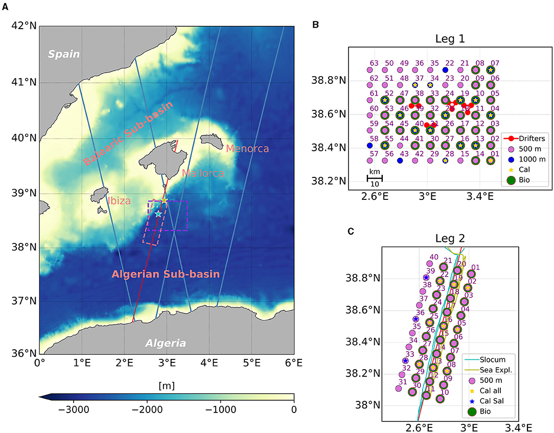
Figure 1. (A) Bathymetric map of the study region. Purple and pink boxes show the regions sampled during Leg 1 and Leg 2, respectively, of the PRE-SWOT field experiment. Blue solid lines represent the limits of future SWOT swaths during the fast-sampling phase. Red line shows the Sentinel-3A ground-track 244 that passed over the Balearic Sea on 13 May 2018. Cyan and green stars represent the position of the Slocum and SeaExplorer gliders, respectively, during the satellite pass. (B) Leg 1 sampling strategy. (C) Leg 2 sampling strategy. Red line represents the Sentinel-3 track 244 passover on 13 May 2018. Cyan and green lines show the routes of the Slocum and SeaExplorer gliders, respectively, following the satellite track from 5 to 14 May 2018. In the legends: Cal and Cal all, water samples collected to calibrate salinity, dissolved oxygen and chl-a fluorescence; Cal Sal, water samples collected to calibrate salinity; Bio, water samples collected for nutrient, pigment signature, and phytoplankton determination; 500 (1,000) m, CTD casts to a maximum depth of 500 (1,000) m.
Leg 2 took place between 13 and 16 May 2018 and focused on completing four transects parallel to Sentinel-3A track 244 that crossed the study region on 13 May 2018 (Figure 1C). For each transect the water column was sampled from the surface to 500 m depth with 10 CTD casts 10 km apart; the transects were separated by 10 km. Water samples for nutrients, pigment signatures and phytoplankton determination were collected in all the rosette casts of the three transects closest to Sentinel-3A track 244 (green dots in Figure 1C). Water samples for calibration of sensors were collected in one cast out of three along these three transects (yellow stars in Figure 1C), while along the western transect only water samples for conductivity calibration were collected (blue stars in Figure 1C). A detailed description of the CTD data processing and calibration can be found in the PRE-SWOT cruise report (Barceló-Llull et al., 2018). We used the Thermodynamic Equations of Seawater (TEOS-10) functions to calculate potential temperature from in situ temperature, and the potential density anomaly (McDougall and Barker, 2011).
2.3. ADCP
Current velocities were continuously recorded using a hull-mounted 75 kHz RDI ADCP at a transit speed of ~8 knots during the two legs of the experiment. The ADCP provided raw data from the surface to ~800 m in bin sizes of 8 and 16 m. The raw data were quality controlled, corrected for heading misalignment and edited with the Common Oceanographic Data Access System (CODAS, Firing et al., 1995). Further details of the ADCP data processing can be found in the PRE-SWOT cruise report (Barceló-Llull et al., 2018).
2.4. Drifters
During Leg 1, twelve surface velocity program (SVP) drifters with a drogue centered at 15 m depth were deployed within the region of study. The aim was to sample frontal areas and study relative dispersion by horizontal stirring at the mesoscale and submesoscale. For that purpose, the drifters were arranged into triangles with a separation between drifters of 5 km (red dots and triangles in Figure 1B). Drifter deployment locations were chosen based on fronts that were visible in ocean color imagery. To remove the inertial signals, the drifter trajectories were filtered using a fifth-order Butterworth low-pass filter with a cutoff of 1.5 times the inertial period of the area, which corresponds to 19 hours (Essink et al., 2019). The zonal and meridional velocity components of each drifter were computed by finite differencing their trajectories.
2.5. Gliders
As part of the PRE-SWOT multi-platform experiment, two underwater gliders followed the Sentinel-3A track 244 (red line in Figures 1A,C): one Slocum from the Balearic Islands Coastal Observing and Forecasting System (SOCIB) and one SeaExplorer from the Mediterranean Institute of Oceanography (MIO). Both gliders were equipped with a pumped CTD sensor (Seabird's GPCTD). The Slocum glider was also equipped with an Anderaa optode for the measurements of dissolved oxygen concentration (O2) and a WetLabs ECO FLNTU for the measurements of chlorophyll-a (chl-a) fluorescence (λEx/λEm: 470/695 nm) and turbidity at 700 nm. The SeaExplorer was equipped with an O2 sensor (Seabird's SBE-43F), from which concentrations are derived, and with a WetLabs ECO FLBBCD for the measurements of chl-a fluorescence (λEx/λEm: 470/695 nm), backscattering at 700 nm (BB700) and humic-like fluorophore fluorescence (λEx/λEm: 370/460 nm). The manufacturer's calibrations were applied to all these sensors. Additionally, the SeaExplorer was equipped with two MiniFluo sensors capable of measuring fluorescent dissolved organic matter (DOM), including organic pollutants such as Polycyclic Aromatic Hydrocarbons (PAHs).
On 3 May 2018, 2 days before the PRE-SWOT cruise started, the Slocum and the SeaExplorer gliders were deployed south of Mallorca. The glider mission plan involved 2 phases. In the first phase, the gliders transited during 2 days between the launch waypoint and the survey start-waypoint (38.94°N, 2.97°E); this phase also served as a test and validation. During the second phase, that extended between 5 and 15 May 2018, the SOCIB glider followed the Sentinel-3A track 244 as closely as possible, whilst the MIO glider sailed 5 km east of the satellite track, in parallel with the SOCIB glider. Over 10 days, both gliders made a round-trip over their respective 100-km long tracks, and finished their missions back at the survey start-waypoint. Glider profiles sampled the water column from the sea surface to a maximum depth of 650 m for both units and were collected at a spatial resolution of about 8 km. Raw glider data from the SOCIB unit were processed with the SOCIB Glider Toolbox, which includes a thermal lag correction (Garau et al., 2011; Troupin et al., 2015). Raw SeaExplorer data were also processed with the SOCIB Glider Toolbox, but at that moment no thermal lag correction was available for the SeaExplorer. We used temperature and salinity observations from the Slocum glider to calculate the dynamic height and compare the scales resolved by the glider with the scales resolved by present altimetric products and CTD observations. To evaluate the impact of vertical velocities on the vertical distribution of tracers, we use chl-a concentrations derived from the SeaExplorer fluorescence measurements and equivalent of a mono-culture of phytoplankton Thalassiosira weissflogii (manufacturer's calibration, https://www.whoi.edu/fileserver.do?id=199125&pt=2&p=207009).
2.6. Satellite Data
The choice of location for sampling of oceanic features was guided and updated in real time by remote sensing imagery during the cruise. Ocean color (OC), SSH, and derived geostrophic currents from remote sensing were essential components of the design of the sampling strategy. The OC data were obtained from the NASA Ocean Color Level 1&2 Browser (https://oceancolor.gsfc.nasa.gov). Level-2 data acquired by both the Moderate Resolution Imaging Spectroradiometer (MODIS) sensor aboard the Aqua satellite, and the Visible and Infrared Imager/Radiometer Suite (VIIRS) sensor carried by the Suomi-NPP satellite were used to design the Leg 1 CTD sampling strategy and the drifter release location. MODIS Level-2 data have a spatial resolution of 1 km, while VIIRS Level-2 data have a spatial resolution of 750 m.
Before and during the cruise, SSH and derived geostrophic currents were obtained from the near-real-time gridded L4 multi-mission altimeter product for the Mediterranean Sea that is distributed by the Copernicus Marine Environment Monitoring Service (CMEMS). After the cruise ended, the reprocessed product had become available. Absolute Dynamic Topography (ADT) was also used to assess the oceanographic context of the experiment. The Mediterranean gridded Level-4 (L4) altimetric products have daily time resolution and 0.125° × 0.125° grid resolution. ADT is computed by adding the mean dynamic topography (MDT) from Rio et al. (2014) to the satellite sea level anomaly (SLA) observations.
We also used 1 Hz along-track level-3 (L3) ADT data collected by the Sentinel-3A satellite mission along the ground-track 244 (cycle 31). This cycle is associated with the passover of the satellite over the Algerian Basin on 13 May 2018 (red line in Figure 1A). We use the reprocessed product for the European Seas distributed by CMEMS with a spatial resolution of 7 km. Cycle 31 is close in time with the glider mission described above: the glider return transects along the Sentinel-3A ground-track were conducted between 9 and 14 May 2018, whilst the satellite overpassed the region on 13 May 2018. Thus, there is a temporal lag < 5 days between the first glider observations on the return transects along the Sentinel-3A ground-track and the satellite overpass. Note that this temporal lag is lower than the temporal lag of 8–11 days that Aulicino et al. (2018) had between observations in their inter-comparison of four SARAL-AltiKa cycles with glider transects in the same region of study. Only data captured between 37.00°N and 39.05°N along the ground-track were extracted in order to achieve close co-location with the glider measurements; this also reduces contamination of the altimetry data due to proximity to the coast (Aulicino et al., 2018). At the time of the satellite passover, the Slocum glider was located at 38.63°N, 2.80°E (cyan star in Figure 1A).
2.7. Optimal Interpolation
Potential temperature, practical salinity, potential density anomaly, and dissolved oxygen concentration (hereafter temperature, salinity, density, and oxygen, respectively) data from Leg 1 were interpolated onto a regular grid with a vertical resolution of 5 m and a horizontal resolution of 2 km. Processed ADCP velocity was vertically smoothed using a Loess filter with a half-power filter cutoff of 60 m and interpolated onto the same regular grid. Optimal interpolation was used for the horizontal interpolation (Bretherton et al., 1976). The data covariance was calculated using a 2D Gaussian function with semimajor and semiminor axes of Lx = Ly = 20 km (see section 3.1.5 for a comparison with the empirical correlation calculated from drifter and CTD observations). With this interpolation, wavelengths smaller than the covariance function correlation lengths (Lx and Ly) are filtered (Pallàs-Sanz et al., 2010). The mean fields are computed from a planar fit for temperature, salinity, density, and oxygen, and are assumed to be constant for ADCP velocity (Rudnick, 1996). The uncorrelated noise for the interpolation of the ADCP velocity is assumed to be 18% of the signal variance; this is estimated as the ratio of noise-to-signal variance considering an instrumental error with a standard deviation of 0.01 m s−1 (Allen et al., 1996; Gomis et al., 2001). The uncorrelated noise for the interpolation of CTD observations is set to 3% of the signal variance (Barceló-Llull et al., 2017); this value is based on instrumental error and the variance of the field. Other authors have used a range of noise-to-signal ratios from 0.01% (Ruiz et al., 2019) to 5% (Rudnick, 1996), in our case we have tested this ratio for different instrumental errors and found that 3% ensures the filtering of noise due to instrumental errors. Note that the observations reconstructed through optimal interpolation are collected during 4.5 days and with this interpolation we assume that they are quasi-synoptic, i.e., a stationary representation of the ocean at the scales resolved of 20 km (e.g., Rudnick, 1996; Pascual et al., 2004; Barceló-Llull et al., 2017; Ruiz et al., 2019).
2.8. Dynamic Height and Geostrophic Velocity Calculation
Dynamic height (DH) and geostrophic velocity fields were computed from the optimally interpolated density data from Leg 1, assuming a reference level of 1,000 m depth (1,010 dbar), the maximum depth of the CTD measurements. DH was also calculated using the Slocum glider transect data. Temperature and salinity measurements collected during the return transect (between 9 and 14 May 2018) were used to compute DH at 30 m depth, as the glider subsurface inflection depth was 15 m and the spatial resolution of glider profiles was low in the shallower layers (Heslop et al., 2017). The reference level for the calculation was set to 650 dbar (maximum depth of the glider measurements). To compare glider and CTD observations from Leg 1, we also computed DH from the optimally interpolated density data, with an assumed reference level of 650 dbar.
Leg 2 CTD data obtained along the four transects parallel to the glider tracks (Figure 1C) were used to compute DH at 30 m depth. In Leg 2, CTD casts sampled the water column down to 500 m depth, and the reference level for the inference of the DH was set to 500 dbar. The DH calculated along the four CTD transects was compared to that computed from the Slocum glider during the return transect, also referenced to 500 dbar for consistency.
The DH calculated from glider data is compared to the ADT obtained from both the Sentinel-3A dataset and the L4 altimetric gridded product. Prior to the comparison, a low-pass Loess filter (Cleveland and Devlin, 1988) with a cutoff of 30 km was applied to the glider, CTD and Sentinel-3A datasets in order to remove measurement noise and small-scale variability (see e.g. Heslop et al., 2017). The efficiency of this approach for the comparison of DH and ADT, and the derived geostrophic velocities, has been demonstrated in previous studies in the same area (Heslop et al., 2017; Aulicino et al., 2018).
2.9. Finite-Size Lyapunov Exponents
Horizontal advection was analyzed using Lagrangian methods, comparing trajectories of in situ and numerical drifters. The trajectories of the numerical drifters were obtained by integrating the horizontal velocity fields derived from the altimetry, CTD, and ADCP observations with a fourth-order Runge-Kutta integrator and a time step of 3 h, assuming time varying altimetric currents and stationary CTD-derived and ADCP velocity fields (d'Ovidio et al., 2013) during the integration period of 6 days. The period of the numerical integration corresponds to the time needed to reach a predefined final separation between numerical drifters. Here we integrated the numerical drifters until they were separated by 45 km, which corresponds to the final separation between in situ drifters after the drifter distance increased exponentially (red lines in Figures 8E,F). The velocity fields were interpolated linearly in space (and in time for the altimetry-derived currents) to the numerical drifter position. The trajectories were used to compute finite-size Lyapunov exponents (FSLEs) (Aurell et al., 1997; Lacorata et al., 2001; d'Ovidio et al., 2004). For clarity, we recall here some basic concepts related to this technique. An FSLE is estimated by finding the time (τ) needed for initially close particles separated by an initial distance d0 at time t0 to reach a prescribed final separation df. The equation that defines an FSLE is the following:
An FSLE, therefore, measures the exponential rate of separation among particle trajectories. It can be computed forward or backward in time. The forward calculation studies the dynamics that drifters initialized nearby undergo in terms of their relative distance. On the other hand, the backward separation is used to estimate regions where water masses far away in the past are brought into contact by the circulation. The points of the line along which these confluence dynamics occur all have relatively high values in maps of FSLEs, and they form what is called Lagrangian fronts (Prants et al., 2014) and belong to the class of Lagrangian Coherent Structures (Haller and Yuan, 2000). Water parcels and arrays of drifters are stretched along Lagrangian fronts, which act as barriers to transport. More details on Lyapunov computation and its meaning can be found in d'Ovidio et al. (2004) and Lehahn et al. (2018).
Backward FSLEs were computed from the numerical trajectories in order to identify Lagrangian fronts (and hence transport barriers) present in the velocity fields derived from altimetry, CTD, and ADCP observations. This was done in order to test whether the trajectories of drifters released during the cruise were aligned along these fronts. For this application, the prescribed initial and final separation distances were optimized for better visualization of the fronts with values of 1 and 20 km, respectively, which are typical values used for this type of application (d'Ovidio et al., 2004; Hernández-Carrasco et al., 2011). This calculation was repeated at different depths (5, 50, 100, and 200 m) using the CTD-derived velocity fields to evaluate the vertical extension of the Lagrangian fronts.
Forward FSLEs were computed in order to compare the exponential rate of separation of numerical and in situ drifters. For a reliable comparison, the initial and final separations used to compute the Lyapunov exponents forward in time from the velocity fields are defined as 7 and 45 km, respectively, which correspond to the separations of in situ drifters for the period in which their relative separation is in an exponential regime (see Figures 8E,F).
2.10. Vertical Velocity Estimation
The quasi-geostrophic (QG) vertical velocity field was calculated through the QG omega equation (Hoskins et al., 1978; Tintoré et al., 1991; Buongiorno Nardelli et al., 2012; Pascual et al., 2015) using the optimally interpolated density field and the derived geostrophic velocity from Leg 1. The QG omega equation is valid for Rossby numbers < < 1 and is presented here in its Q vector form:
where
w is the vertical velocity, ugeo is the geostrophic velocity vector, ρ is density, ρ0 is the mean density, N2 is the Brunt–Väisälä frequency (), f is the Coriolis parameter, considered constant and computed at the mean latitude, and g is gravity. In this implementation, N2 only depends on depth and is estimated as the horizontal average of the Brunt–Väisälä frequency estimated at each grid point. The Q vector represents the deformation of the horizontal density gradient by the geostrophic velocity field. The forcing term of the QG omega equation is on the right-hand side of (2), while on the left-hand side an elliptic operator is applied to the vertical velocity. The QG omega equation is solved by applying an iterative relaxation method with Dirichlet boundary conditions (w = 0).
2.11. Oceanographic Context From Satellites and Sampling Region Determination
During the month before the PRE-SWOT experiment, ocean color images provided essential information at high resolution for the design of the experiment. However, observations without cloud-coverage in the area of study were limited to some specific days. Figures 2A–C show three examples of the best observations of ocean color preceding the PRE-SWOT experiment. On 17 April 2018, relatively high values of chl-a of the order of 0.3 mg m−3 were observed in an elongated meander at ~2.50°E, 38.00°N extending to the northeast (Figure 2A). Three days after, the chl-a signal was concentrated at ~3.20°E, 38.60°N and had values similar to those observed in the region southeast of Mallorca and south of Menorca (Figure 2B). Two days before the cruise experiment, this signal was displaced to ~2.90°E, 38.50°N; this map was used to determine the position of the CTD casts in Leg 1 and the drifter release locations (Figure 2C).
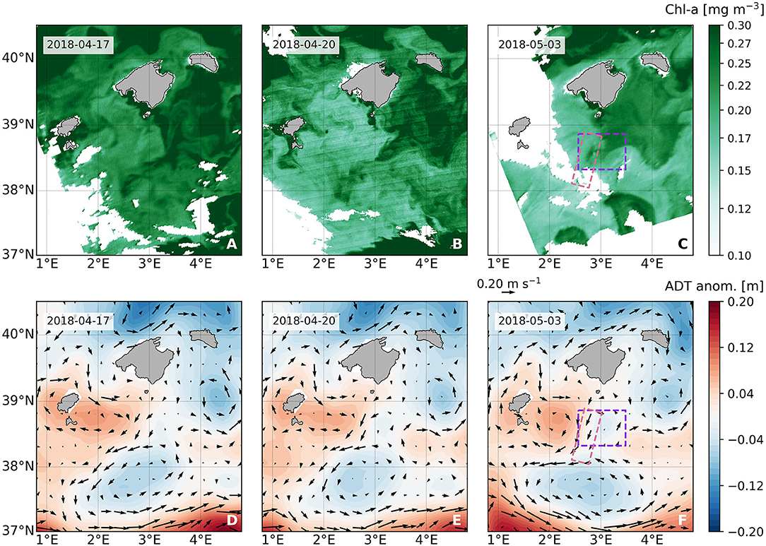
Figure 2. (A–C) Ocean color images on different dates in the region of study. Data from MODIS were used on 17 April and 3 May 2018, while VIIRS data were used on 20 April 2018. (D–F) Absolute dynamic topography anomaly and altimetric geostrophic velocities on different dates in the region of study. For clarity, only one out of two current vectors are plotted. Purple and pink boxes in (C,F) delimit the regions sampled during Leg 1 and Leg 2 of the PRE-SWOT experiment, respectively.
According to altimetric observations, the target sampling area (boxes in Figure 2C) was surrounded by three oceanographic features: a cyclonic eddy in the Algerian basin, a cyclonic eddy south of Menorca, and an anticyclonic eddy east of Ibiza (Figures 2D–F). The western part of the region with the chl-a signal observed at ~2.90°E, 38.50°N on 3 May 2018 (Figure 2C) was characterized by southwestern velocities of the order of 0.20 m s−1 during the month before the cruise experiment. The persistence of the meandering flow and the presence of an associated front visible on ocean color maps determined the region selected for the cruise experiment within the domain that will be sampled by SWOT during the fast-sampling phase. Note that ocean color maps (Figures 2A–C) reveal the presence of filaments, eddies and fronts that are not detected in present-day altimetric observations (Figures 2D–F). The in situ sampling is then expected to provide information at high resolution which is out of reach of present-day altimeters but potentially detectable by future SWOT observations.
3. Results
3.1. Hydrodynamic Signature of a Meandering Front
3.1.1. Hydrological Characterization
Maps of salinity at different depths from the Leg 1 CTD sampling reveal the presence of a meandering front in the upper layers that separates saltier water at the northeastern edge of the domain from fresher water at the southeastern edge (Figures 3A,E). The signal of the front in salinity is apparent from the surface to ~150 m depth (not shown), having a difference of 0.8 between maximum and minimum salinity values at 5 m, the shallowest layer of CTD observations, that decreases with depth. The map of temperature at 5 m depth (Figure 3B) is characterized by a meridional distribution with warmer water at the western edge and colder water at the eastern edge of the sampled domain. Below 5 m and until ~150 m, the temperature signal resembles the front with colder water in the northeastern part of the domain and warmer water in the southeastern part (Figure 3F). The front detected between 5 and ~150 m depth is characterized by saltier and colder water on the northeastern side that is the signal of surface local Atlantic Water (local AW)—AW already modified by a long residence in the Mediterranean. On the southeastern side the front has fresher and warmer water that is the signature of recent Atlantic Water (recent AW) coming from the Strait of Gibraltar (Barceló-Llull et al., 2019). In this depth layer, density is dominated by salinity over thermal effects (Figures 3C,G). At 5 m depth, dissolved oxygen is maximum at the saltier side of the front, with concentration values of 7.54 mg l−1 (Figure 3D). West of 3.00°E the concentration is minimum reaching values of 7.29 mg l−1. The dissolved oxygen distribution at 50 m depth does not seem related to the front (Figure 3H).
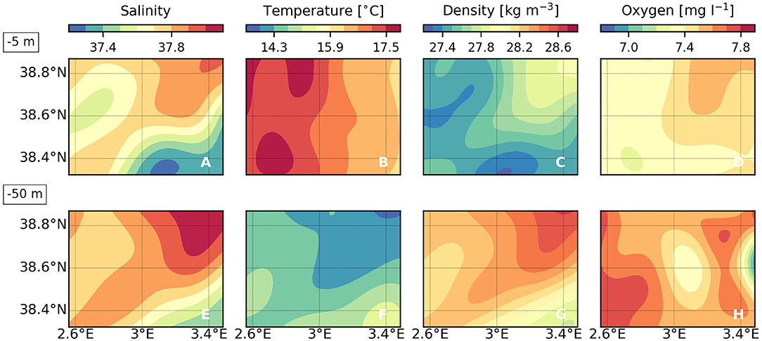
Figure 3. Salinity, temperature, density, and oxygen maps at (A–D) 5 and (E–H) 50 m depth from Leg 1 CTD data.
3.1.2. Water Masses
To analyse the different water masses residing in the region of study, temperature-salinity diagrams of all the CTD profiles from Leg 1 are shown in Figure 4. A local maximum of temperature and salinity between 200 and 400 m depth reveals the presence of Levantine Intermediate water (LIW), and temperature values between 12.7°C and 12.9°C are the signal of Western Mediterranean Deep water (WMDW) (Pinot et al., 2002; Balbín et al., 2012; Barceló-Llull et al., 2019). Western Mediterranean Intermediate water (WMIW), associated with a relative minimum of temperature at intermediate layers, is not observed in the sampled region. At ~50 m depth some profiles of saltier and colder local AW have higher concentrations of oxygen than the other profiles (Figure 4A), which may be the signal of a local process of oxygenation. A maximum of dissolved oxygen is normally formed above the deep chlorophyll maximum as a result of photosynthetic activity by phytoplankton cells. This has been observed in the northwestern Mediterranean by Estrada et al. (1999), Segura-Noguera et al. (2016), and Lefevre (2019). Between 300 and 500 m depth, higher temperature and salinity values are associated with lower oxygen concentration (Figure 4B). At depths higher than 500 m, the oxygen concentration is almost constant.
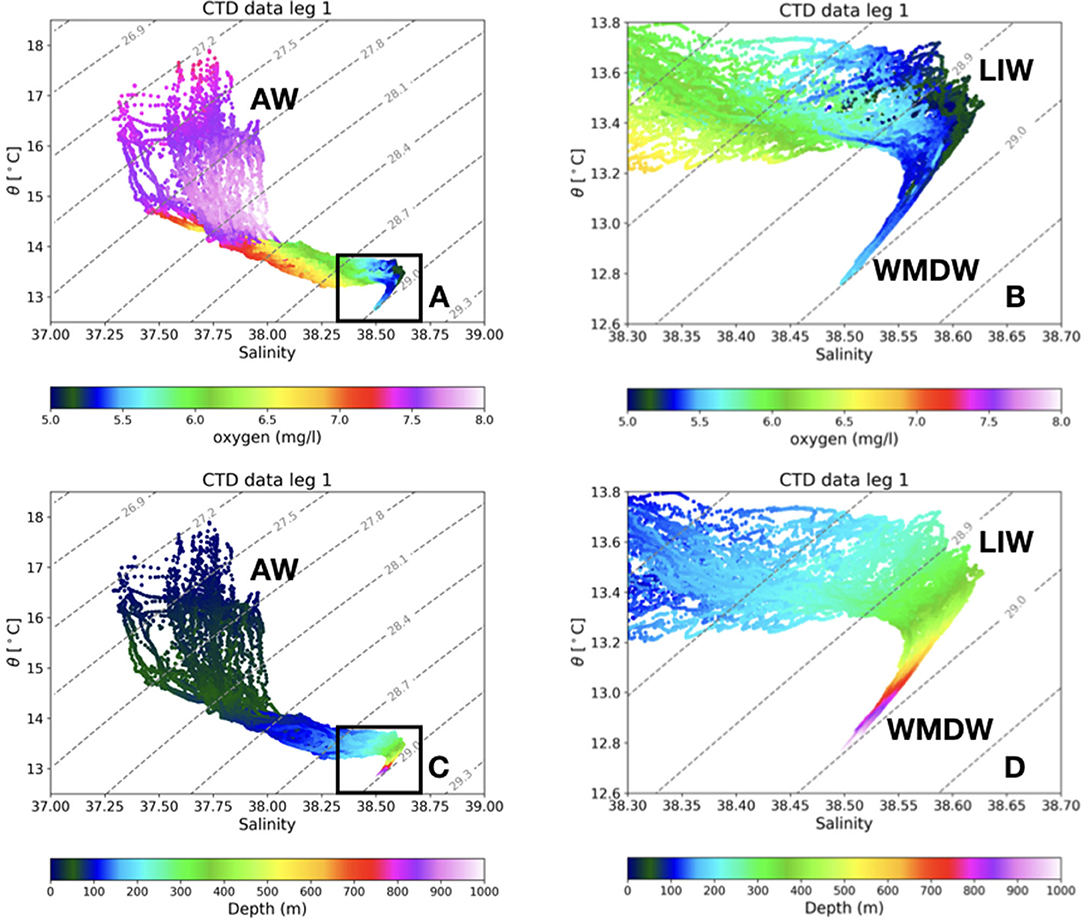
Figure 4. (A–D) Temperature-salinity diagrams using data from Leg 1 CTD profiles. Color in top (bottom) plots represents the oxygen concentration (depth). The right column is a zoom of the left column. The presence of the following water masses is also indicated: Atlantic water (AW), Levantine Intermediate water (LIW), and Western Mediterranean Deep water (WMDW).
3.1.3. Geostrophic and Ageostrophic Horizontal Velocities
Geostrophic velocities calculated from CTD observations (ugeo) at 20 m depth reveal a meandering flow coming from the center north of the domain and changing its direction to the east with a maximum speed of the order of 0.20 m s−1 (Figure 5A, black arrows). The southeastern part of the domain is characterized by a northeastward flow reaching a maximum speed of 0.26 m s−1, whilst the western part shows an anticyclonic circulation with maximum speeds of the order of 0.15 m s−1. The ADCP velocity (uadcp), that includes the geostrophic and ageostrophic components of the flow, at 20 m depth shows a similar circulation with differences in direction in the southeastern and northwestern regions of the domain (Figure 5A, cyan arrows). The geostrophic currents derived from altimetry (ualt; Figure 5B) do not resolve the features that the ugeo and uadcp maps show. This is due to the lower effective spatial resolution of altimetric gridded products in the Mediterranean (~130 km wavelength, Ballarotta et al., 2019) in comparison with CTD and ADCP observations (~20 km wavelength) that limits the representation of the circulation in the region. Even the general circulation pattern shown in the altimetric map does not correspond to the higher-resolution in situ velocity fields. Only in the western side of the domain, where a southwestward flow dominates the circulation, ualt have similarities with ugeo and uadcp. A visual comparison with the trajectories of the drifters released during the cruise also highlights the limitations of present-day altimetry (see drifter trajectories in Figure 5). The geostrophic velocity calculated from CTD data and the total ADCP horizontal velocity show good agreement with the trajectories followed by the drifters, while altimetric currents cannot explain their eastward displacement.
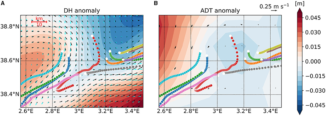
Figure 5. (A) Dynamic height (DH) anomaly at 5 m depth and geostrophic velocity vectors (in black) at 20 m depth (for consistency with ADCP velocity) calculated using CTD data from Leg 1. ADCP velocity vectors at 20 m depth are plotted in cyan. For clarity, only one out of two current vectors are plotted. (B) Absolute dynamic topography (ADT) anomaly computed from CMEMS altimetry gridded products on 3 May 2018 and derived geostrophic velocity vectors. All velocity vectors are plotted with the same scale. Dots show the trajectories followed by the drifters released during the PRE-SWOT experiment for the period 5–13 May; white dots are the release positions, and the time period between each drifter location is 2 h.
To compare quantitatively the drifter movement with ualt, ugeo and uadcp, we have estimated the meridional and zonal velocity components of each drifter from their trajectories between 5 and 12 May 2018. Table 1 shows the Pearson correlation coefficients obtained between each component of the drifter velocity and the corresponding component of the altimetric, geostrophic and ADCP velocities. The zonal component (u) of the drifter velocity has similar correlation coefficients with the three velocity fields and is maximum with the geostrophic velocity (0.90). The meridional component (v) has a correlation coefficient of 0.59 with the altimetric meridional component that increases with the ADCP (0.70) and geostrophic (0.75) velocities. Hence, among the three datasets, the geostrophic velocity field calculated from CTD data is the one showing the best agreement with the trajectories followed by drifters. This result suggests that the strongest component of the horizontal currents responsible for the drifter displacement is geostrophic, and hence potentially resolvable in higher-resolution altimetric maps like the ones that SWOT should provide.
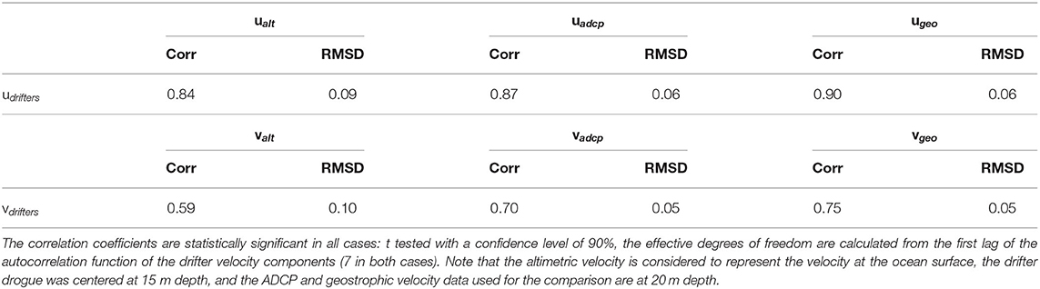
Table 1. Correlation coefficients (Corr) and root mean square differences (in m s−1, RMSD) between the zonal and meridional components of the drifter velocity and the same components of the altimetric, ADCP and geostrophic velocities interpolated onto the drifter position (altimetric velocity was previously interpolated in time along the drifter time axis).
Regarding the vertical distribution of horizontal velocities, zonal sections of the meridional component of the ADCP velocity (vadcp) show good correspondence with the meridional component of the geostrophic velocity (vgeo) calculated from CTD observations (Figure 6). However, ADCP velocity has higher magnitude and vertical variability than the geostrophic velocity field. Vertical profiles of the root mean square difference (RMSD) show that the differences in magnitude are higher in the upper layers and decrease with depth, in correspondence with the decrease in magnitude of both velocities. The correlation coefficient vertical profiles reveal that both fields have maximum correlation in the upper ~150 m depth, where the front is located. The correlation decreases with depth, where the vertical variability of the ADCP velocity is more evident in comparison with the smoother geostrophic velocity. Dashed (dotted) lines in Figure 6 represent the RMSD and correlation coefficient vertical profiles between the meridional (zonal) components of both velocity fields considering all data in each depth layer. The zonal components have higher RMSD and lower correlation coefficient than the meridional components of the velocities. This translates in higher differences between the zonal velocities along meridional sections (not shown) than between the meridional velocities along the zonal transects shown in Figure 6. Hence, the effect of having more synoptic observations along meridional transects than along zonal transects does not imply smaller differences between ADCP and geostrophic velocity fields. This is due to the optimal interpolation used to reconstruct the observations, which considers all data in each depth layer. Note that these velocities are obtained from two independent instruments and following different procedures, hence, different sources of error may contribute to the small differences observed between both velocity fields. First, the geostrophic velocity calculated from CTD data may be underestimated as it is calculated assuming a level of no motion of 1,000 m, while the ADCP velocity does not have this constraint and also includes the barotropic component of the horizontal velocity, which may increase its magnitude. In addition, from 500 to 1,000 m depth the number of CTD casts is reduced and this could imply an additional smoothing to the interpolated fields. Also, the ADCP velocity field has smaller features on the southeastern and northwestern corners of the domain (Figure 5A) that could be due to (i) the higher resolution along meridional transects of ADCP data compared to the lower resolution of CTD stations, and (ii) potential artifacts of the optimal interpolation close to the boundaries that may affect the estimation of the derivatives involved in the computation of ugeo. Lastly, the ADCP velocity has more vertical variability (Figure 6) that could be the signal of errors coming from the instrument. In addition to the different sources of error, the ADCP velocity may include ageostrophic motions that are not represented in the geostrophic velocity field, such as the cyclostrophic component that could have a contribution in areas of strong curvature, internal waves and inertial motions (Pallàs-Sanz and Viúdez, 2005; Morrow et al., 2019). The small differences observed between ADCP and CTD-derived geostrophic velocities, with maximum RMSD of the order of 0.06 m s−1 and correlation coefficients of ~0.9 in the upper layers, and the different sources of error that may introduce these differences, suggest that the geostrophic component of the horizontal flow may dominate the local dynamics of this region down to scales of 20 km.
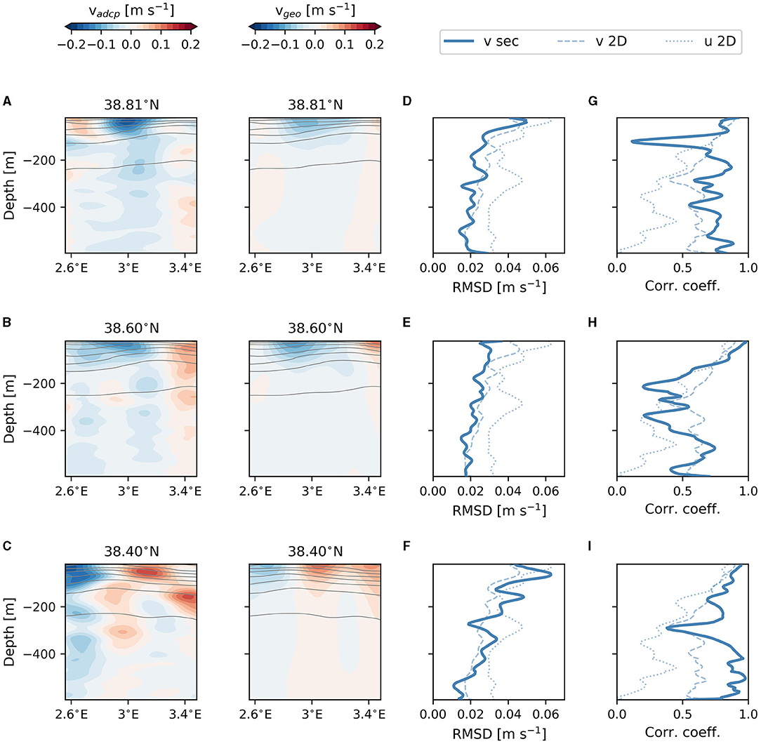
Figure 6. Zonal sections along (A) 38.81°N, (B) 38.60°N, and (C) 38.40°N of the meridional component of the optimally interpolated ADCP velocity and geostrophic velocity calculated from CTD data. Gray contours represent the potential density anomaly (the contour at the bottom is the 29.0 kg m−3 isoline and density decreases upwards with a contour interval of 0.2 kg m−3). Solid lines in (D–F) are the vertical profiles of the root mean square differences (RMSD) between both velocity fields along (D) 38.81°N, (E) 38.60°N, and (F) 38.40°N. Solid lines in (G–I) are the vertical profiles of the correlation coefficient between the corresponding velocity fields. Dashed (dotted) lines represent the vertical profiles of the RMSD (D–F) and correlation coefficient (G–I) between the meridional (zonal) velocity components considering all data in each depth layer.
The vertical relative vorticity field scaled by the planetary vorticity, or Rossby number, has been estimated from ugeo (Rog) and from uadcp (Ro). Both fields have similar distributions and intensities with small differences due to the deviations observed between velocity fields (Figure 7). Good correspondence between both fields is observed below 20 m depth (not shown), with a higher decrease with depth of the Rog magnitude due to the smoother ugeo field (Figure 6). Ro has values ranging from −0.26 to 0.20 and Rog between −0.24 and 0.32 in the region of study and at the scales resolved of ~20 km, in accordance with a dominance of the geostrophic component of the flow in this region for the period analyzed. Note that with higher-resolution observations we would sample smaller-scale features and the Rossby number would potentially be higher. Hence, all our estimates are based on the scales we resolve of ~20 km.
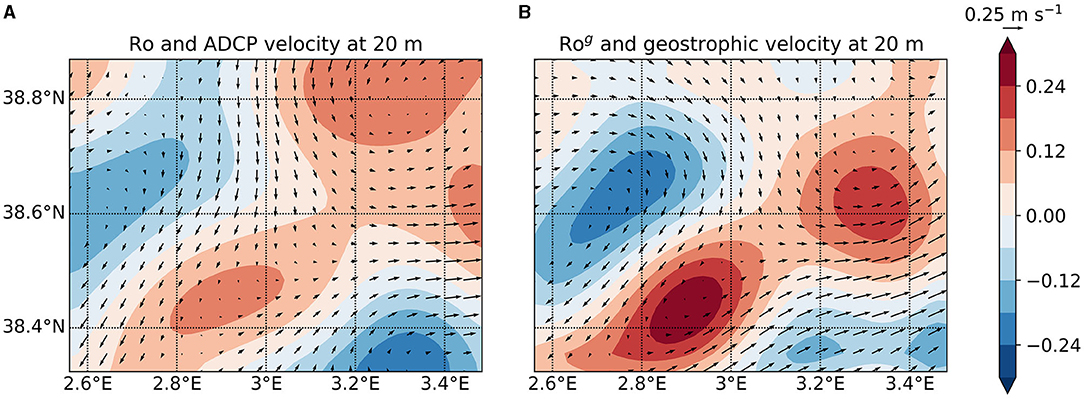
Figure 7. Maps at 20 m depth of (A) Ro with ADCP velocity vectors and (B) Rog with geostrophic velocity vectors. For clarity, only one out of two current vectors are plotted.
3.1.4. Finite-Size Lyapunov Exponents
The backward Lyapunov exponents computed from ualt, ugeo and uadcp are shown in Figures 8A–C. Over the Lagrangian fronts we plot the trajectories of two drifters launched in situ on 8 May 2018. After their release, the two drifters moved away from their deployment locations, marking an increasing separation with time (Figure 8E). The behavior of the two drifters particularly underlines the classical presence of a so-called hyperbolic point in the velocity field (e.g., see Figure 3 in Lehahn et al., 2007): the drifters separate along an imaginary line, sometimes referred to as a Lagrangian front or as a Lagrangian Coherent Structure (Haller and Yuan, 2000; Prants et al., 2014). The FSLE maps estimated from ugeo and uadcp (Figures 8B,C) confirm this suggestion (d'Ovidio et al., 2004), while the Lagrangian fronts derived from ualt (Figure 8A) are inconsistent with the trajectories of the two drifters, even in qualitative terms. The eastern drifter in particular crosses an altimetry-derived Lagrangian front, which is supposed to behave as a transport barrier. The situation is different for the case of the CTD- and ADCP-derived Lyapunov exponents, which display a better agreement between Lagrangian fronts and drifter trajectories. Indeed, the trajectory of the two drifters is consistent with an expected separation along the attracting front underlined by CTD- and ADCP-derived Lyapunov exponents (Figures 8B,C). The Lagrangian front detected in the CTD-derived Lyapunov exponents appears to extend vertically and vanish approximately at 200 m depth (Figure 8D).
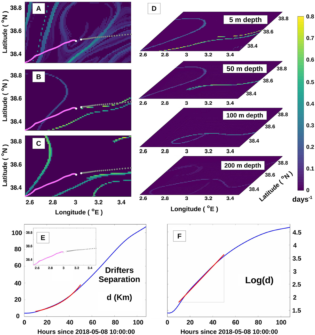
Figure 8. (A–C) Backward finite-size Lyapunov exponent maps computed from (A) altimetry-, (B) CTD-, and (C) ADCP-derived velocity fields on 8 May 2018. These maps show the Lagrangian fronts computed from the altimetry-derived velocity at the surface, the CTD geostrophic velocity at 20 m depth, and the ADCP velocity at 20 m depth, respectively. Pink and gray dots represent the trajectories of two drifters released on 8 May 2018 during the PRE-SWOT experiment and whose release positions are indicated by the white dots. (D) Maps of the finite-size Lyapunov exponents computed from the CTD-derived velocity field at different depth layers (5, 50, 100, and 200 m depth). (E,F) Estimation of the exponential rate of separation for the two drifters shown in (A–C). (E) Temporal evolution of the distance (d) that separates both drifters. The drifters' trajectories are displayed by the gray and pink dots in the inset plot. (F) Semi-logarithmic scale of the separation distance evolution with time [log(d)]. The red line represents the linear regression for the logarithmic scale corresponding to the red curve in (E) which, in turn, represents the exponential separation of the drifters for the period between 10 and 50 h since the release time of these two drifters.
In order to compare the exponential rate of separation computed from the in situ drifter trajectories and the numerical drifters, we proceeded in the following steps. We firstly identified a temporal window over which the relative separation between the two drifters is approximately exponential. This temporal window extends from 10 to 50 h since 8 May 2018 at 10:00:00 (Figures 8E,F). We then used the initial and final separations corresponding to the extrema of this temporal window (7 and 45 km, respectively) to recompute the finite-size Lyapunov exponents from the velocity fields by simulating the trajectories of numerical drifters. The corresponding ualt, ugeo and uadcp finite-size Lyapunov exponents, recomputed in this area over the Lagrangian fronts, are shown in Table 2. The exponential rate of separation for the in situ drifters is 1.097 days−1. Altimetry again has the largest mismatch with respect to the in situ drifters, grossly underestimating their rate of separation by more than 50%. CTD- and ADCP-derived exponential rates of separations are closer to the one of the in situ drifters.
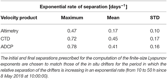
Table 2. Maximum, mean, and standard deviation (STD) of the forward finite-size Lyapunov exponents of the altimetry-, CTD-, and ADCP-derived Lagrangian fronts.
3.1.5. Vertical Velocities and Impact on Biochemical Variability
The horizontal distribution of the QG vertical velocity field (wQG) is similar throughout the upper 300 m depth and is characterized by an upwelling cell at the southern edge of the domain (3.05°E, 38.42°N) surrounded by two downwelling cells at 3.28°E, 38.48°N and 2.85°E, 38.53°N (Figure 9A). At 85 m depth wQG has maximum values ranging between −7.7 and 7.9 m day−1. However, a sensitivity test reveals the dependence of the extreme values of wQG to the correlation scales used to interpolate the original density field (Table 3). An increase of the correlation scales from 20 to 25 km would induce a decrease on the extreme values of wQG of about 50%. Note that applying smaller correlation scales (within the range allowed by the sampling) in the optimal interpolation enables the representation of smaller-scale variability in the interpolated fields, and this may include higher ageostrophic and divergent motions that would translate to larger vertical velocities, consistent with the results from the sensitivity test. A criterion used to define the correlation scales is the estimation of the empirical correlation (Gomis et al., 2001; Pascual et al., 2004). Figure 10 shows the correlation of the original density field at 100 m depth, and the correlation of the drifter velocities (which have higher resolution than the CTD casts). The Gaussian function that visually better resembles the empirical correlations is likely to be the one with a characteristic scale of 20 km, especially for the meridional component of the drifter velocity and for density. This analysis supports the correlation scales used in the optimal interpolation.
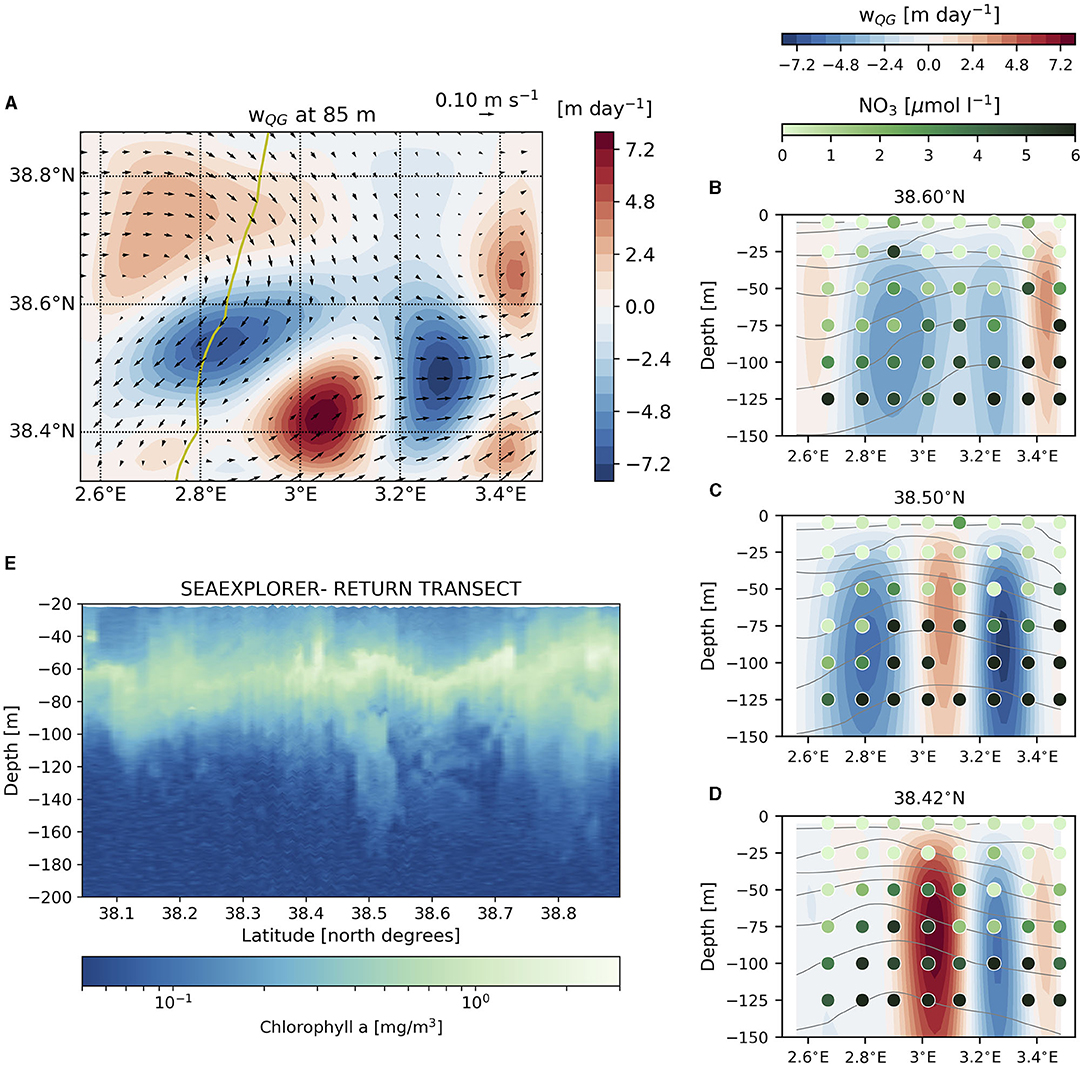
Figure 9. (A) Map at 85 m depth of the QG vertical velocity field and geostrophic velocity vectors calculated from CTD data (for clarity, only one out of two current vectors are plotted). Green line represents the return trajectory of the SeaExplorer glider along which the chlorophyll-a concentration is shown in E. (B–D) Zonal sections of the QG vertical velocity field along (A) 38.60°N, (B) 38.50°N, and (C) 38.42°N with the nitrate concentration sampled at the closest stations along (A) 38.59°N, (B) 38.50°N, and (C) 38.41°N. Gray contours represent the potential density anomaly along the same sections as the QG vertical velocity (the contour at the bottom is the 28.8 kg m−3 isoline and density decreases upwards with a contour interval of 0.2 kg m−3). (E) Chlorophyll-a concentration derived from the SeaExplorer measurements along the return transect.
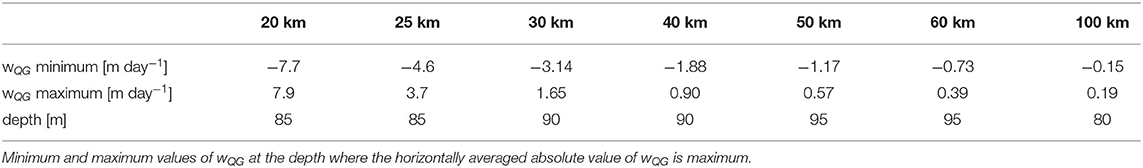
Table 3. Sensitivity test of wQG to the correlation scales used in the optimal interpolation of the original density field.
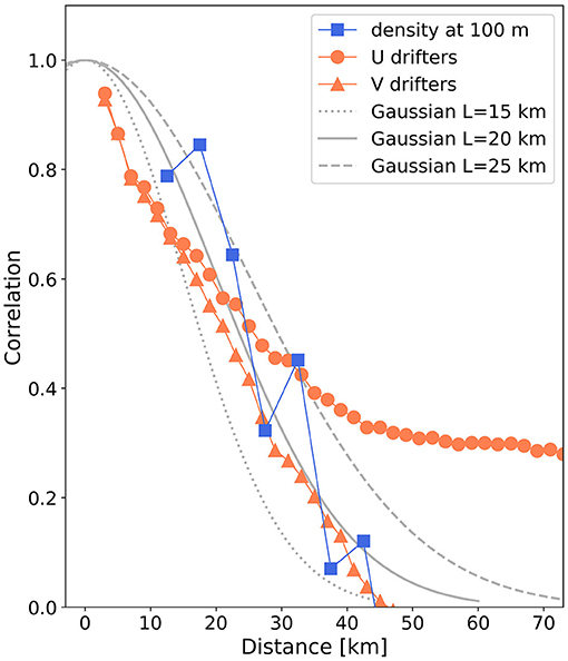
Figure 10. Correlation between data pairs that are separated by a defined distance (x-axis) and considering a bin size of 5 km for the original density from Leg 1 at 100 m depth (blue squares), and considering a bin size of 2 km for the zonal and meridional components of the drifter velocity (orange dots and triangles, respectively). As an example, the first square is the correlation of those density data pairs that have a separation between 10 and 15 km. Gray dotted, solid, and dashed lines represent three Gaussian functions with standard deviations of 15, 20, and 25 km, respectively. The Gaussian function that resembles better the empirical correlations is likely the Gaussian with a standard deviation of 20 km, and this is the correlation scale used to interpolate the original fields from Leg 1.
The spatial variability of nitrate and chl-a concentrations is consistent with the vertical velocity field calculated from CTD data (Figures 9B–E). An enhancement of nitrate concentration within the photic layer was detected at some stations located close to the upwelling cell: concentrations higher than ~5 μmol l−1 at ~75 m are found in the 38.42°N and 38.50°N zonal sections at the stations located at ~2.90°E and ~3.00°E, and also in the 38.50°N zonal section at the station located at ~3.10°E (Figures 9C,D). This enhanced concentration of nitrate within the photic layer may indicate a recent input of nutrients from deeper layers induced by the upwelling cell centered at 3.05°E, 38.42°N (Figure 9A). A vertical section of chl-a concentration from the SeaExplorer glider return transect shows higher values between 100 and 180 m depth than in the surroundings at ~2.85°E, 38.50°N. This may be the signal of a chl-a subduction related to the western downwelling cell centered at 2.84°E, 38.53°N.
3.2. Scales Detected by the Slocum Glider Along the Sentinel-3A Track
3.2.1. Glider Data vs. Altimetry Data
Figure 11 shows the along-track ADT from the Sentinel-3A satellite mission and the DH computed from glider observations, together with the ADT from the gridded altimetric products interpolated onto the glider transect. The glider DH partially captures the signature of two positive anomalies located south of the Balearic Islands at ~38.00°N and ~38.50°N. These two features are located around 0.5 degrees apart in longitude, thus, the length scale resolved by the glider data in this region has a radius of ~13 km, the same order of magnitude of the Rossby radius of deformation in the western Mediterranean Sea (Escudier et al., 2016; Barceló-Llull et al., 2019). Not surprisingly, these two signatures are not captured by the gridded ADT interpolated onto the glider transect (brown line in Figure 11) due to both its lower spatial resolution and the correlation length scale applied to construct the gridded product (100 km). In consequence, the gridded ADT anomaly shows one single positive anomaly and does not resolve the variability at the glider scales. The Sentinel-3A ADT properly represents the signal of these two positive anomalies with some differences in amplitude and position with respect to the signals detected in glider data. The amplitude of the northern signature is higher in Sentinel-3A ADT anomaly while the opposite occurs in the southern feature. In addition, the maximum anomalies of both fields are slightly displaced and the length scale solved by the Sentinel-3A dataset decreases to ~8 km. The glider completed the transect in almost 6 days so these differences may be due to the time lag between the Sentinel-3A and glider observations. A vertical line in Figure 11 shows the location of the glider during the Sentinel-3A overpass. North and south of this point the glider sampling has a time difference varying from hours to days with respect to the Sentinel-3A sampling as we approach to the limits of the transect. This fact explains the discrepancies in height of up to 2.5 cm observed in the southern feature, and also the displacement of its maximum, captured by both platforms.
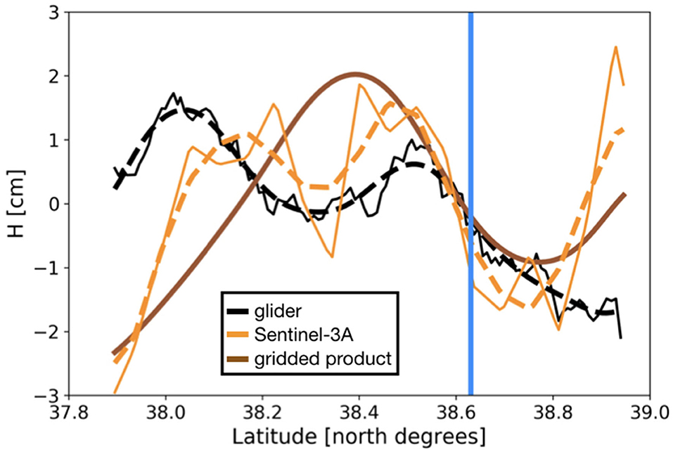
Figure 11. Filtered (dashed black thick line) and unfiltered (solid black thin line) DH from glider data along ground-track 244 associated with the date of passage of the Sentinel-3A satellite over the Algerian Basin on 13 May 2018. Filtered (dashed orange thick line) and unfiltered (solid orange thin line) ADT from the Sentinel-3A along-track European reprocessed product, and ADT computed from the Mediterranean Sea reprocessed altimetry gridded product (brown line). Since the reference level used to compute the DH is different from the reference level used in altimetry, the mean value of each variable has been removed to better compare all variables. The blue vertical line shows the location of the glider during the Sentinel-3A overpass.
3.2.2. Glider and CTD Dynamic Height
To evaluate the contribution of the deeper layers on the estimation of DH, Figure 12A shows the DH computed using Leg 1 CTD data interpolated onto the glider track and assuming the reference level at 650 dbar (orange line) and 1,000 dbar (blue line). The mean values of DH are subtracted to compare the variability of both lines, which is almost identical with an absolute maximum around 38.60°N and minimum values at the bounds of the transect. Thus, the contribution of the water column between 650 and 1,000 m depth to the computed DH is a constant value that increases the absolute value of DH, but does not change the horizontal variability. As a conclusion, in the study area, the contribution of the deeper layers in the DH anomaly can be considered negligible.
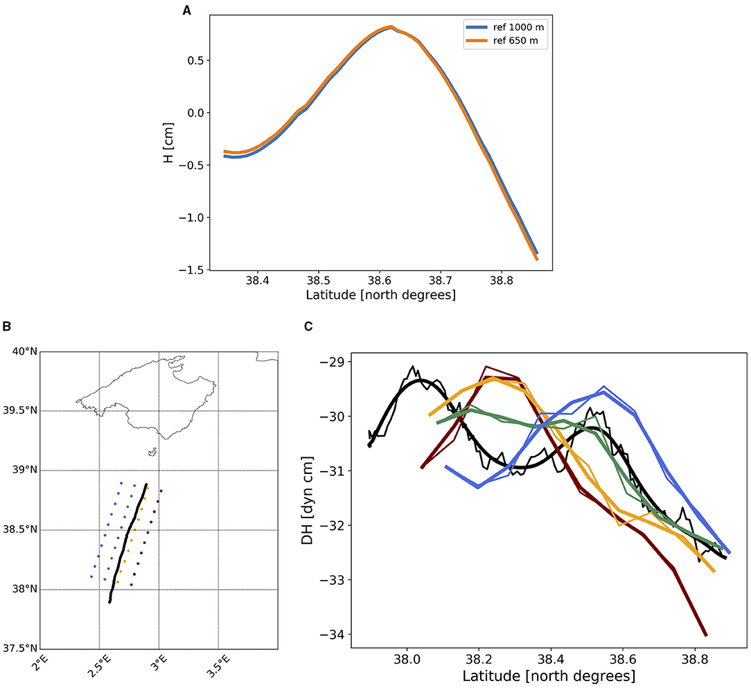
Figure 12. (A) DH computed from the optimally interpolated CTD data (Leg 1) interpolated onto the glider track and assuming a reference level of 1,000 dbar (blue line) and 650 dbar (orange line). The mean values of DH are subtracted for the comparison. (B) CTD casts collected during Leg 2 along four transects parallel to the glider track (black line, 9–14 May 2018): transect 1 (red dots, 16 May 2018), transect 2 (yellow dots, 15 May 2018), transect 3 (green dots, 14–15 May 2018), and transect 4 (blue dots, 13–14 May 2018). (C) DH computed from glider (black line) and CTD data (same color code as in B), both computed assuming a reference level at 500 dbar and smoothed with a 30 km low-pass Loess filter. Thin lines show DH computed using the unfiltered glider and CTD data.
The DH computed using the Slocum glider return data is compared to the DH calculated from Leg 2 CTD data along the four transects parallel to the glider track (Figures 12B,C). Overall, the DH shows weak features with magnitudes ranging between 2 and 3 cm from both platform observations. The spatiotemporal variability of the circulation in the region of study introduces the differences observed between the four CTD transects, as they are sampled in different locations and times. The fine-scale signal detected by both platforms shows an evolution between transect 4, sampled on 13-14 May 2018, and transect 1, sampled on 16 May 2018. The maximum of DH located at ~38.50°N in transect 4 and in the glider data is displaced to ~38.25°N in transects 2 and 1. The CTD DH more similar to the glider DH is the one computed along transect 3 (green line in Figure 12C). Both have similar values from 38.50°N toward the north, even though the data have been collected ~10 km apart. The reason of this similarity is that both platforms sampled the region almost simultaneously and they could capture the same signature. Note that even if transect 3 DH has similar values than glider DH north of 38.50°N, transect 4 has a maximum of DH located at the same latitude as the glider data. The DH calculated using transect 2 CTD data (yellow line in Figure 12C) shows a different signal than the signature observed by the glider due to the difference in time of both samplings, even though data were collected along the same track.
4. Discussion and Conclusions
We have analyzed the impact of the scales resolved by different observational platforms on the representation of the horizontal velocity field associated with a meandering front observed from the surface to ~150 m depth. We compared the surface geostrophic velocity field obtained from present-day altimetric products with (i) the geostrophic velocity calculated from CTD measurements, (ii) the total horizontal velocity measured by the ADCP and (iii) drifter trajectories. The CTD-derived geostrophic velocity and ADCP horizontal velocity have similar distributions with maximum root mean square differences between both fields of the order of 0.06 m s−1 and correlation coefficients of ~0.9 in the upper layers (Figure 6). The differences between ADCP and geostrophic velocities could be attributed to different sources of error that arise from the different instruments and procedures used to obtain these fields: level of no motion used to calculate the geostrophic velocity, reduced number of CTD casts between 500 and 1,000 m depth, higher resolution of ADCP data along meridional transects, errors associated with the optimal interpolation, and presence of internal waves and inertial motions in the ADCP velocity field. The small differences observed between both fields, with maximum RMSD of the order of 0.06 m s−1, and the different sources of error that may introduce these differences, suggest that the geostrophic component of the horizontal flow may dominate the local dynamics of this region down to scales of 20 km. The Rossby number computed from each velocity field has absolute values lower than 0.32 at the scales resolved by the sampling (20 km wavelength). The present-day resolution of altimetric products precludes estimation of the horizontal velocities obtained from the ADCP and CTD sampling at scales of ~20 km. This is corroborated by the dispersion of drifters released within the study region: while the CTD-derived and ADCP velocities are in good agreement with the drifter trajectories, the altimetric currents cannot justify their eastward displacement. Quantitatively, the CTD-derived geostrophic velocity has a higher correlation with the drifter velocities than the other fields. This suggests that the geostrophic velocity calculated from CTD observations, which are sampled with a resolution similar to the target SWOT resolution, correctly represents the actual currents that drive the drifters over the sampling domain. In addition, note that the CTD and ADCP observations reconstructed through optimal interpolation are collected during 4.5 days, and they are assumed to be quasi-synoptic to apply the interpolation (e.g., Rudnick, 1996; Pascual et al., 2004; Barceló-Llull et al., 2017; Ruiz et al., 2019). This approximation may introduce errors to the reconstructed fields and derived variables due to the lack of synopticity of the observations (Allen et al., 2001; Gomis et al., 2005). The correspondence detected between the trajectory of in situ drifters and the CTD-derived and ADCP velocity fields supports the approximation of quasi-synoptic observations in the PRE-SWOT experiment.
The Lagrangian analysis performed by comparing the relative separation of in situ drifters with the numerical drifters derived from the assumed stationary CTD and ADCP velocity fields is quite consistent in showing that the region of study has strong frontogenetic dynamics. Interestingly, these dynamics fall into a “dark spot” for altimetry due to its resolution limitations. More specifically, the FSLEs derived from the CTD and ADCP velocity fields are high (reaching maximum values of 0.72 and 0.78 days−1, which is typical of boundary currents estimated from altimetry: see e.g., Figure 1 in Hernández-Carrasco et al., 2012), and approximately double that measured from altimetry in this region. The exponential rate of separation estimated for two in situ drifters is similar to the CTD- and ADCP-derived FSLE maximum values, while nadir altimetry FSLEs misrepresent this value. In addition, the position of the Lagrangian front detected in the ADCP- and CTD-derived FSLE maps is consistent with the in situ drifter trajectories, while the altimetry-derived Lagrangian front, that should represent a transport barrier, is crossed by the eastern in situ drifters. The results from the Lagrangian analysis support the approximation of quasi-synoptic observations considered to optimally interpolate the CTD and ADCP observations, and the assumption of stationary velocity fields used to integrate the numerical drifters. We consider that the approximation of stationarity is applicable in our PRE-SWOT Lagrangian analysis because (i) the duration of the integration is short (6 days or less) and (ii) we are not analyzing eddy retention but only the position and intensity of Lagrangian fronts (d'Ovidio et al., 2013). We are looking forward to future satellite missions like SWOT to have synoptic, time-varying maps of the circulation at these spatial scales. For Lagrangian studies, these future observations will allow us to explore the evolution in time of transport barriers, and see the implication of their dynamics in terms of biogeochemistry and biodiversity, possibly testing hypotheses that at the moment can only be analyzed on modeled experiments (e.g., Lévy et al., 2015).
The rapid relative separation of two drifters along the FSLE front indicates that horizontal stirring stretches any tracer present in the region along that front. The estimation of the backward FSLE along the Lagrangian front provides in fact the intensity of the convergent dynamics acting in the direction orthogonal to the front, and hence the rate at which the passive tracer gradients intensify. The presence of these frontogenetic dynamics induced by horizontal stirring is consistent with the presence of the density gradient, which is the source of the vertical velocities derived through the QG omega equation, as well as with the front visible in the satellite-derived chl-a images. Note that ADCP- and CTD-derived FSLEs provide similar results. This observation suggests again that the dynamics of this region are mostly in geostrophic balance. The Lagrangian front observed during our field experiment is an example of what we seek to resolve in the near future from high-resolution altimetric observations that SWOT is expected to provide, and that today is only accessible from in situ observations.
The vertical velocity field was calculated through integration of the QG omega equation using the CTD-derived geostrophic velocity and density fields. The wQG distribution is characterized by an upwelling cell surrounded by two downwelling cells with a magnitude that is maximum at ~ 85 m depth and decreases downward and upward. The magnitude of wQG depends on the correlation scales used to interpolate the original fields. Using correlation scales of 20 km, wQG has maximum and minimum values of 7.9 m day−1 and −7.7 m day−1, respectively. With correlation scales larger than 30 km the magnitude decreases more than 60% for minimum values and 80% for maximum values. The Gaussian function that is most similar to the empirical correlations, estimated using the original density CTD data and both components of the drifter velocities, is that with a standard deviation of 20 km, supporting the choice of spatial scales used for the optimal interpolation. We have analyzed the spatial variability of nitrate and chl-a in relation to the vertical velocity field. An enhancement of nitrate concentration within the photic layer was detected at two stations located close to the upwelling cell. This may indicate a recent input of nutrients from deeper layers induced by the upwelling cell. Chl-a concentration derived from SeaExplorer glider measurements had high values at ~2.85°E, 38.50°N between 100 and 180 m depth. This may be the signal of a subduction of chl-a related to the western downwelling cell centered at 2.84°E, 38.53°N.
The DH estimated from glider observations shows the signature of two positive anomalies separated by 0.5 degree in longitude (Figure 11), thus, the length scale resolved by the glider data has a radius of ~13 km, the same order of magnitude of the Rossby radius of deformation in the western Mediterranean Sea (Escudier et al., 2016; Barceló-Llull et al., 2019). While the altimetric gridded ADT does not capture this variability due to its lower spatial resolution and the correlation length scale applied to construct the product, the Sentinel-3A ADT correctly represents the signal of these two positive anomalies, with some differences in amplitude and position with respect to the signals detected by the glider. The positive anomalies detected in the Sentinel-3A ADT and glider DH are slightly displaced, and the length scale resolved by the Sentinel-3A dataset decreases to ~8 km. These differences may be due to the time lag between the glider and Sentinel-3A observations.
A comparison between the CTD and glider observations reveals the temporal variability of the estimated DH, which changes over the four transects sampled in Leg 2. The CTD transect with a DH variability similar to that calculated from glider observations was the one that sampled the water column almost simultaneously with the glider, even though they were 10 km apart. The two CTD transects that had a larger time lag with respect to the glider observations have larger differences in DH variability. A sensitivity test of the DH estimated using CTD observations down to 650 and 1,000 m shows that the contribution of the deeper layers is an almost constant mean value and does not introduce significant horizontal variability. In the same region of study, Aulicino et al. (2018) previously obtained similar results from a DH sensitivity test calculated by assuming different reference levels between 200 and 900 m depth. This suggests that, when a quasi-synoptic sampling is needed, in the study region CTD casts do not need to sample the water column down to 1,000 m depth in order to estimate DH. This has the advantage that it is possible to sample small study regions more quickly.
We have used in situ observations from different observational platforms to demonstrate the limitations of present-day nadir altimetry to resolve the circulation in a region of the western Mediterranean Sea with relatively moderate dynamic activity (Figure 2). The altimetric observations are too coarse to capture the evolving circulation over the period of the cruise: some features are missing, others are misplaced, and most are significantly weaker than in the in situ observations. One important consequence is that dispersion processes are incorrectly represented, as evidenced by the drifter experiment. This misrepresentation of lateral stirring results in data suggesting much weaker fronts. As a consequence, the frontogenetic region sampled during the PRE-SWOT cruise, which has a clear signal in biochemistry, has almost no signal in altimetric maps. The implication is that, at present, we must use in situ instruments to characterize the physical signatures of the features we have surveyed. Interestingly, the component which is missing in the horizontal circulation captured by nadir altimetry appears to be mainly geostrophic down to scales of 20 km wavelength in the region of study and during the sampling period, and hence it should be resolvable by future altimetric satellites with higher-resolution such as SWOT. At smaller scales it is expected that it will be a significant departure from geostrophy and, therefore, other satellite missions measuring ocean surface currents are required (Gommenginger et al., 2019).
The integrated multi-platform and interdisciplinary sampling of the region south of the Balearic Islands has revealed interesting results about the potential scales that may be resolved by SWOT, and also the limitations of current nadir altimetry. Our study quantifies and shows that the geostrophic approximation at scales of 20 km in the region of study is a good approximation. We have also calculated the QG vertical velocity field and detected a correspondence with the spatial distribution of nitrate and chl-a concentrations. Through the multi-platform and interdisciplinary PRE-SWOT experiment in collaboration with the French campaign PROTEVSMED-SWOT, we have evaluated (i) the 3D dynamics of the study region, which has been previously scarcely sampled with only some recent studies using high-resolution glider data (Heslop et al., 2017; Aulicino et al., 2018), and (ii) the coupling between fine-scale physics and biological measurements (Tzortzis et al., 2021). With this joint experiment we have evaluated the dynamics of the western Mediterranean SWOT crossover and gained experience in multi-institution and multi-platform campaign coordination.
The Mediterranean Sea has lower first Rossby radius of deformation (~5–15 km, Beuvier et al., 2012; Escudier et al., 2016; Barceló-Llull et al., 2019; Kurkin et al., 2020) than other regions of the global ocean at mid-latitudes (~20–40 km, Chelton et al., 1998). This means that the spatial scales are smaller and nadir altimetry only captures a small part of the mesoscale dynamics. Hence, in this region SWOT is expected to provide a substantial improvement in the observation of these scales (d'Ovidio et al., 2019). In addition, the Mediterranean Sea is characterized by low tides and relatively weak internal wave dynamics that make this region interesting for interdisciplinary studies (d'Ovidio et al., 2019). Note that due to the particular characteristics of the Mediterranean Sea, the conclusions from this study are not extendable to other regions with different dynamics.
In future experiments, it may be interesting to explore the region northwest of the Balearic Islands, which has been documented to have higher dynamic activity than the region studied here and is under the SWOT path during the fast-sampling phase. In future work, we will use high-resolution regional ocean circulation models to conduct Observing System Simulation Experiments to (i) evaluate the quasi-synopticity of the observations collected in multi-platform experiments similar to PRE-SWOT, (ii) compare the optimal interpolation with other methods of reconstruction that can account for the temporal variability of the observations, and (iii) study optimal sampling strategies for multi-platform experiments aimed at SWOT validation.
Data Availability Statement
The datasets presented in this study can be found in online repositories. The names of the repository/repositories and accession number(s) can be found below: http://dx.doi.org/10.20350/digitalCSIC/8640.
Author Contributions
BB-L led the writing of the manuscript. AP designed, obtained the funding for and led the PRE-SWOT experiment. BB-L, AS-R, and EC post-processed the in situ observations. FD and GF conducted the Lagrangian analysis. All authors contributed to the analysis of the results and in the collection of the in situ observations.
Funding
The PRE-SWOT experiment was funded by the Spanish Research Agency and the European Regional Development Fund (AEI/FEDER, UE) under Grant Agreement (CTM2016-78607-P). BB-L was supported by a postdoctoral contract in the framework of the EuroSea project that has received funding from the European Union's Horizon 2020 research and innovation programme under Grant Agreement No. 862626. This study is also a contribution to the SWOT Science Team (TOSCA-CNES VERSO and TOSCA-CNES BIOSWOT-AdAC project proposals) and to the EuroSea project (Horizon 2020 research and innovation programme under Grant Agreement No. 862626).
Conflict of Interest
The authors declare that the research was conducted in the absence of any commercial or financial relationships that could be construed as a potential conflict of interest.
Publisher's Note
All claims expressed in this article are solely those of the authors and do not necessarily represent those of their affiliated organizations, or those of the publisher, the editors and the reviewers. Any product that may be evaluated in this article, or claim that may be made by its manufacturer, is not guaranteed or endorsed by the publisher.
Acknowledgments
We express our gratitude to the technical staff (UTM-CSIC) and crew of the R/V García del Cid for supporting our work at sea and to Andrea Cabornero, Esther Capó, Noemí Calafat, Tim Toomey, Juan Gabriel Herná́ndez, David Roque, Albert Miralles, Manuel Rubio, and Marc Torner for their participation in the acquisition of the observations. We thank SOCIB staff for the MIO's glider deployment.
References
Allen, J., Smeed, D., Crisp, N., Ruiz, S., Watts, S., Vélez, P., et al. (1996). Upper Ocean Underway Operations on BIO Hesperides Cruise OMEGA-ALGERS (Cruise 37) Using SeaSoar and ADCP 30/9/96 - 14/10/96. Southampton Oceanography Centre.
Allen, J. T., and Smeed, D. A. (1996). Potential vorticity and vertical velocity at the Iceland- Færœs Front. J. Phys. Oceanogr. 26, 2611–2634. doi: 10.1175/1520-0485(1996)026<2611:PVAVVA>2.0.CO;2
Allen, J. T., Smeed, D. A., Nurser, A. J. G., Zhang, J. W., and Rixen, M. (2001). Diagnosis of vertical velocities with the QG omega equation: an examination of the errors due to sampling strategy. Deep Sea Res. 48, 315–346. doi: 10.1016/S0967-0637(00)00035-2
Aulicino, G., Cotroneo, Y., Ruiz, S., Sánchez Román, A., Pascual, A., Fusco, G., et al. (2018). Monitoring the algerian basin through glider observations, satellite altimetry and numerical simulations along a saral/altika track. J. Mar. Syst. 179, 55–71. doi: 10.1016/j.jmarsys.2017.11.006
Aurell, E., Boffetta, G., Crisanti, A., Paladin, G., and Vulpiani, A. (1997). Predictability in the large: an extension of the concept of lyapunov exponent. J. Phys. A Math. Gen. 30, 1–26. doi: 10.1088/0305-4470/30/1/003
Balbín, R., Flexas, M. M., López-Jurado, J. L., Pe na, M., and Alemany, F. (2012). Vertical velocities and biological consequences at a front detected at the Balearic Sea. Cont. Shelf Res., 47, 28–41. doi: 10.1016/j.csr.2012.06.008
Ballarotta, M., Ubelmann, C., Pujol, M.-I., Taburet, G., Fournier, F., Legeais, J.-F., et al. (2019). On the resolutions of ocean altimetry maps. Ocean Sci. 15, 1091–1109. doi: 10.5194/os-15-1091-2019
Barceló-Llull, B., Mason, E., Capet, A., and Pascual, A. (2016). Impact of vertical and horizontal advection on nutrient distribution in the southeast Pacific. Ocean Sci. 12, 1003–1011. doi: 10.5194/os-12-1003-2016
Barceló-Llull, B., Pallás-Sanz, E., Sangrá, P., Martínez-Marrero, A., Estrada-Allis, S. N., and Arístegui, J. (2017). Ageostrophic secondary circulation in a subtropical intrathermocline Eddy. J. Phys. Oceanogr. 47, 1107–1123. doi: 10.1175/JPO-D-16-0235.1
Barceló-Llull, B., Pascual, A., Día-Barroso, L., Sánchez-Román, A., Casas, B., Muñoz, C., et al. (2018). PRE-SWOT Cruise Report. Mesoscale and Sub-Mesoscale Vertical Exchanges from Multi-Platform Experiments and Supporting Modeling Simulations: Anticipating SWOT Launch (CTM2016-78607-P). Technical report, CSIC. doi: 10.20350/digitalCSIC/8584
Barceló-Llull, B., Pascual, A., Ruiz, S., Escudier, R., Torner, M., and Tintoré, J. (2019). Temporal and spatial hydrodynamic variability in the mallorca channel (western Mediterranean sea) from 8 years of underwater glider data. J. Geophys. Res. Oceans 124, 2769–2786. doi: 10.1029/2018JC014636
Baschek, B., and Farmer, D. M. (2010). Gas bubbles as oceanographic tracers. J. Atmos. Ocean. Technol. 27, 241–245. doi: 10.1175/2009JTECHO688.1
Beuvier, J., Béranger, K., Lebeaupin Brossier, C., Somot, S., Sevault, F., Drillet, Y., et al. (2012). Spreading of the western mediterranean deep water after winter 2005: time scales and deep cyclone transport. J. Geophys. Res. Oceans 117:C7. doi: 10.1029/2011JC007679
Bishop, S. P., Small, R. J., and Bryan, F. O. (2020). The global sink of available potential energy by mesoscale air-sea interaction. J. Adv. Model. Earth Syst. 12:e2020MS002118. doi: 10.1029/2020MS002118
Bouffard, J., Pascual, A., Ruiz, S., Faugére, Y., and Tintoré, J. (2010). Coastal and mesoscale dynamics characterization using altimetry and gliders: a case study in the Balearic Sea. J. Geophys. Res. 115:C10029. doi: 10.1029/2009JC006087
Boy, F., Desjonquéres, J., Picot, N., Moreau, T., and Raynal, M. (2017). Cryosat-2 sar-mode over oceans: processing methods, global assessment, and benefits. IEEE Trans. Geosci. Remote Sens. 55, 148–158. doi: 10.1109/TGRS.2016.2601958
Bretherton, F. P., Davis, R. E., and Fandry, C. B. (1976). A technique for objective analysis and design of oceanographic experiments applied to MODE-73. Deep Sea Res. 23, 559–582. doi: 10.1016/0011-7471(76)90001-2
Buongiorno Nardelli, B. (2020). A multi-year time series of observation-based 3d horizontal and vertical quasi-geostrophic global ocean currents. Earth Syst. Sci. Data 12, 1711–1723. doi: 10.5194/essd-12-1711-2020
Buongiorno Nardelli, B., Guinehut, S., Pascual, A., Drillet, Y., Ruiz, S., and Mulet, S. (2012). Towards high resolution mapping of 3-D mesoscale dynamics from observations. Ocean Sci. 8, 885–901. doi: 10.5194/os-8-885-2012
Chelton, D. B., deSzoeke, R. A., Schlax, M. A., El Naggar, K., and Siwertz, N. (1998). Geographical variability of the first-baroclinic Rossby radius of deformation. J. Phys. Oceanogr. 28, 433–460. doi: 10.1175/1520-0485(1998)028<0433:GVOTFB>2.0.CO;2
Chelton, D. B., Schlax, M. A., and Samelson, R. M. (2011). Global observations of nonlinear mesoscale eddies. Prog. Oceanogr. 91, 167–216. doi: 10.1016/j.pocean.2011.01.002
Cleveland, W. S., and Devlin, S. J. (1988). Locally weighted regression: an approach to regression analysis by local fitting. J. Am. Stat. Assoc. 83, 596–610. doi: 10.1080/01621459.1988.10478639
Cotroneo, Y., Aulicino, G., Ruiz, S., Pascual, A., Budillon, G., Fusco, G., et al. (2016). Glider and satellite high resolution monitoring of a mesoscale eddy in the algerian basin: effects on the mixed layer depth and biochemistry. J. Mar. Syst. 162, 73–88. doi: 10.1016/j.jmarsys.2015.12.004
D'Asaro, E., Lee, C., Rainville, L., Harcourt, R., and Thomas, L. (2011). Enhanced turbulence and energy dissipation at ocean fronts. Science 332, 318–322. doi: 10.1126/science.1201515
D'Asaro, E. A., Carlson, D. F., Chamecki, M., Harcourt, R. R., Haus, B. K., Fox-Kemper, B., et al. (2020). Advances in observing and understanding small-scale open ocean circulation during the Gulf of Mexico research initiative era. Front. Mar. Sci. 7:349. doi: 10.3389/fmars.2020.00349
D'Asaro, E. A., Shcherbina, A. Y., Klymak, J. M., Molemaker, J., Novelli, G., Guigand, C. M., et al. (2018). Ocean convergence and the dispersion of flotsam. Proc. Natl. Acad. Sci. U.S.A. 115, 1162–1167. doi: 10.1073/pnas.1718453115
d'Ovidio, F., Fernández, V., Hernández-Garcia, E., and López, C. (2004). Mixing structures in the Mediterranean Sea from finite-size Lyapunov exponents. Geophys. Res. Lett. 31:17. doi: 10.1029/2004GL020328
d'Ovidio, F., Monte, S. D., Penna, A. D., Cotté, C., and Guinet, C. (2013). Ecological implications of eddy retention in the open ocean: a Lagrangian approach. J. Phys. A Math. Theoret. 46:254023. doi: 10.1088/1751-8113/46/25/254023
d'Ovidio, F., Pascual, A., Wang, J., Doglioli, A. M., Jing, Z., Moreau, S., et al. (2019). Frontiers in fine-scale in situ studies: opportunities during the SWOT fast sampling phase. Front. Mar. Sci. 6:168. doi: 10.3389/fmars.2019.00168
Dufau, C., Orsztynowicz, M., Dibarboure, G., Morrow, R., and Le Traon, P.-Y. (2016). Mesoscale resolution capability of altimetry: present and future. J. Geophys. Res. Oceans 121, 4910–4927. doi: 10.1002/2015JC010904
Escudier, R., Renault, L., Pascual, A., Brasseur, P., Chelton, D., and Beuvier, J. (2016). Eddy properties in the western mediterranean sea from satellite altimetry and a numerical simulation. J. Geophys. Res. Oceans 121, 3990–4006. doi: 10.1002/2015JC011371
Essink, S., Hormann, V., Centurioni, L. R., and Mahadevan, A. (2019). Can we detect submesoscale motions in drifter pair dispersion? J. Phys. Oceanogr. 49, 2237–2254. doi: 10.1175/JPO-D-18-0181.1
Estrada, M., Varela, R. A., Salat, J., Cruzado, A., and Arias, E. (1999). Spatio-temporal variability of the winter phytoplankton distribution across the Catalan and North Balearic fronts (NW Mediterranean). J. Plankton Res. 21, 1–20. doi: 10.1093/plankt/21.1.1
Firing, E., Ranada, J., and Caldwell, P. (1995). Processing ADCP Data with the CODAS Software System Version 3.1. Joint Institute for Marine and Atmospheric Research, University of Hawaii &National Oceanographic Data Center.
Freilich, M., and Mahadevan, A. (2021). Coherent pathways for subduction from the surface mixed layer at ocean fronts. J. Geophys. Res. Oceans 126:e2020JC017042. doi: 10.1029/2020JC017042
Fu, L.-L., and Ferrari, R. (2008). Observing oceanic submesoscale processes from space. EOS Trans. AGU 89:488. doi: 10.1029/2008EO480003
Fu, L.-L., and Ubelmann, C. (2014). On the transition from profile altimeter to swath altimeter for observing global ocean surface topography. J. Atmos. Ocean. Technol. 31, 560–568. doi: 10.1175/JTECH-D-13-00109.1
Garau, B., Ruiz, S., Zang, G. W., Heslop, E., Kerfoot, J., Pascual, A., et al. (2011). Thermal lag correction on Slocum CTD glider data. J. Atmos. Ocean. Technol. 28, 1065–1071. doi: 10.1175/JTECH-D-10-05030.1
Gómez-Navarro, L., Cosme, E., Sommer, J., Papadakis, N., and Pascual, A. (2020). Development of an image de-noising method in preparation for the surface water and ocean topography satellite mission. Remote Sens. 12:734. doi: 10.3390/rs12040734
Gomis, D., Pascual, A., and Pedder, M. A. (2005). Errors in dynamical fields inferred from oceanographic cruise data: Part II. The impact of the lack of synopticity. J. Mar. Syst. 56, 334–351. doi: 10.1016/j.jmarsys.2005.02.003
Gomis, D., Ruiz, S., and Pedder, M. A. (2001). Diagnostic analysis of the 3D ageostrophic circulation from a multivariate spatial interpolation of CTD and ADCP data. Deep Sea Res. I Oceanogr. Res. Pap. 48, 269–295. doi: 10.1016/S0967-0637(00)00060-1
Gommenginger, C., Chapron, B., Hogg, A., Buckingham, C., Fox-Kemper, B., Eriksson, L., et al. (2019). SEASTAR: a mission to study ocean submesoscale dynamics and small-scale atmosphere-ocean processes in coastal, shelf and polar seas. Front. Mar. Sci. 6:457. doi: 10.3389/fmars.2019.00457
Haller, G., and Yuan, G. (2000). Lagrangian coherent structures and mixing in two-dimensional turbulence. Phys. D Nonlinear Phenomena 147, 352–370. doi: 10.1016/S0167-2789(00)00142-1
Hernández-Carrasco, I., López, C., Hernández-Garcia, E., and Turiel, A. (2011). How reliable are finite-size lyapunov exponents for the assessment of ocean dynamics? Ocean Modell. 36, 208–218. doi: 10.1016/j.ocemod.2010.12.006
Hernández-Carrasco, I., López, C., Hernández-Garcia, E., and Turiel, A. (2012). Seasonal and regional characterization of horizontal stirring in the global ocean. J. Geophys. Res. Oceans 117:C10. doi: 10.1029/2012JC008222
Heslop, E. E., Sánchez-Román, A., Pascual, A., Rodriguez, D., Reeve, K. A., Faugére, Y., et al. (2017). Sentinel-3a views ocean variability more accurately at finer resolution. Geophys. Res. Lett. 44, 12367–12374. doi: 10.1002/2017GL076244
Hoskins, B. J., Draghici, I., and Davies, H. C. (1978). A new look at the ω-equation. Q. J. R. Met. Soc. 104, 31–38. doi: 10.1002/qj.49710443903
Klein, P., Lapeyre, G., Siegelman, L., Qiu, B., Fu, L.-L., Torres, H., et al. (2019). Ocean-scale interactions from space. Earth Space Sci. 6, 795–817. doi: 10.1029/2018EA000492
Kurkin, A., Kurkina, O., Rybin, A., and Talipova, T. (2020). Comparative analysis of the first baroclinic Rossby radius in the Baltic, Black, Okhotsk, and Mediterranean seas. Russ. J. Earth Sci. 20:ES4008. doi: 10.2205/2020ES000737
Kwon, Y.-O., Alexander, M. A., Bond, N. A., Frankignoul, C., Nakamura, H., Qiu, B., et al. (2010). Role of the gulf stream and kuroshio-oyashio systems in large-scale atmosphere-ocean interaction: a review. J. Clim. 23, 3249–3281. doi: 10.1175/2010JCLI3343.1
Lacorata, G., Aurell, E., and Vulpiani, A. (2001). Drifter dispersion in the adriatic sea: Lagrangian data and chaotic model. Ann. Geophys. 19, 121–129. doi: 10.5194/angeo-19-121-2001
Le Traon, P. Y. (2013). From satellite altimetry to argo and operational oceanography: three revolutions in oceanography. Ocean Sci. 9, 901–915. doi: 10.5194/os-9-901-2013
Lefevre, B. (2019). Seasonal patterns of chlorophyll and biogeochemistry in the Balearic channels: a multiplatform approach (Master's thesis). University Sorbonne, Paris, France.
Lehahn, Y., d'Ovidio, F., and Koren, I. (2018). A satellite-based lagrangian view on phytoplankton dynamics. Annu. Rev. Mar. Sci. 10, 99–119. doi: 10.1146/annurev-marine-121916-063204
Lehahn, Y., d'Ovidio, F., Lévy, M., and Heifetz, E. (2007). Stirring of the northeast atlantic spring bloom: a Lagrangian analysis based on multisatellite data. J. Geophys. Re. Oceans 112:C8. doi: 10.1029/2006JC003927
Lévy, M., Franks, P. J. S., and Smith, K. S. (2018). The role of submesoscale currents in structuring marine ecosystems. Nat. Commun. 9:4758. doi: 10.1038/s41467-018-07059-3
Lévy, M., Jahn, O., Dutkiewicz, S., Follows, M. J., and d'Ovidio, F. (2015). The dynamical landscape of marine phytoplankton diversity. J. R. Soc. Interface 12:20150481. doi: 10.1098/rsif.2015.0481
Lévy, M., Klein, P., and Treguier, A. M. (2001). Impact of sub-mesoscale physics on production and subduction of phytoplankton in an oligotrophic regime. J. Mar. Res. 59, 535–565. doi: 10.1357/002224001762842181
Ma, X., Jing, Z., Chang, P., Liu, X., Montuoro, R., Small, R. J., et al. (2016). Western boundary currents regulated by interaction between ocean eddies and the atmosphere. Nature 535, 533–537. doi: 10.1038/nature18640
Mahadevan, A. (2016). The impact of submesoscale physics on primary productivity of plankton. Annu. Rev. Mar. Sci. 8, 161–184. doi: 10.1146/annurev-marine-010814-015912
Mahadevan, A., Pascual, A., Rudnick, D. L., Ruiz, S., Tintoré, J., and D'Asaro, E. (2020). Coherent pathways for vertical transport from the surface ocean to interior. Bull. Am. Meteorol. Soc. 101, E1996–E2004. doi: 10.1175/BAMS-D-19-0305.1
Mahadevan, A., and Tandon, A. (2006). An analysis of mechanisms for submesoscale vertical motion at ocean fronts. Ocean Modell. 14, 241–256. doi: 10.1016/j.ocemod.2006.05.006
McDougall, T. J., and Barker, P. M. (2011). Getting Started with TEOS-10 and the Gibbs Seawater (GSW) Oceanographic Toolbox. SCOR/IAPSO WG127, 28.
Morrow, R., Fu, L.-L., Ardhuin, F., Benkiran, M., Chapron, B., Cosme, E., et al. (2019). Global observations of fine-scale ocean surface topography with the surface water and ocean topography (SWOT) mission. Front. Mar. Sci. 6:232. doi: 10.3389/fmars.2019.00232
Pallás-Sanz, E., Johnston, T. M. S., and Rudnick, D. L. (2010). Frontal dynamics in a California Current System shallow front: 1. Frontal processes and tracer structure. J. Geophys. Res. 115, 1–14. doi: 10.1029/2009JC006032
Pallás-Sanz, E., and Viúdez, A. (2005). Diagnosing mesoscale vertical motion from horizontal velocity and density data. J. Phys. Oceanogr. 35, 1744–1762. doi: 10.1175/JPO2784.1
Pascual, A., Gomis, D., Haney, R. L., and Ruiz, S. (2004). A quasigeostrophic analysis of a meander in the Palamos Canyon: vertical velocity, geopotential tendency, and a relocation technique. J. Phys. Oceanogr. 34, 2274–2287. doi: 10.1175/1520-0485(2004)034<2274:AQAOAM>2.0.CO;2
Pascual, A., Ruiz, S., Buongiorno Nardelli, B., Guinehut, S., Iudicone, D., and Tintoré, J. (2015). Net primary production in the Gulf Stream sustained by quasi-geostrophic vertical exchanges. Geophys. Res. Lett. 42, 441–449. doi: 10.1002/2014GL062569
Pascual, A., Ruiz, S., Olita, A., Troupin, C., Claret, M., Casas, B., et al. (2017). A multiplatform experiment to unravel meso- and submesoscale processes in an intense front (AlborEx). Front. Mar. Sci. 4:39. doi: 10.3389/fmars.2017.00039
Pietri, A., Capet, X., d'Ovidio, F., Levy, M., Sommer, J. L., Molines, J.-M., et al. (2021). Skills and limitations of the adiabatic omega equation: how effective is it to retrieve oceanic vertical circulation at mesoscale and submesoscale? J. Phys. Oceanogr. 51, 931–954. doi: 10.1175/JPO-D-20-0052.1
Pinot, J.-M., López-Jurado, J. L., and Riera, M. (2002). The CANALES experiment (1996-1998). Interannual, seasonal, and mesoscale variability of the circulation in the Balearic Channels. Prog. Oceanogr. 55, 335–370. doi: 10.1016/S0079-6611(02)00139-8
Pollard, R. T., and Regier, L. A. (1992). Vorticity and vertical circulation at an ocean front. J. Phys. Oceanogr. 22, 609–625. doi: 10.1175/1520-0485(1992)022<0609:VAVCAA>2.0.CO;2
Prants, S., Budyansky, M., and Uleysky, M. (2014). Identifying lagrangian fronts with favourable fishery conditions. Deep Sea Res. I Oceanogr. Res. Pap. 90, 27–35. doi: 10.1016/j.dsr.2014.04.012
Raney, R. K. (1998). The delay/doppler radar altimeter. IEEE Trans. Geosci. Remote Sens. 36, 1578–1588. doi: 10.1109/36.718861
Rio, M.-H., Pascual, A., Poulain, P.-M., Menna, M., Barceló, B., and Tintoré, J. (2014). Computation of a new mean dynamic topography for the mediterranean sea from model outputs, altimeter measurements and oceanographic in situ data. Ocean Sci. 10, 731–744. doi: 10.5194/os-10-731-2014
Rudnick, D. L. (1996). Intensive surveys of the Azores Front: 2. Inferring the geostrophic and vertical velocity fields. J. Geophys. Res. Oceans 101, 16291–16303. doi: 10.1029/96JC01144
Ruiz, S., Claret, M., Pascual, A., Olita, A., Troupin, C., Capet, A., et al. (2019). Effects of oceanic mesoscale and submesoscale frontal processes on the vertical transport of phytoplankton. J. Geophys. Res. Oceans 124, 5999–6014. doi: 10.1029/2019JC015034
Ruiz, S., Pascual, A., Garau, B., Faugére, Y., Alvarez, A., and Tintoré, J. (2009). Mesoscale dynamics of the Balearic Front, integrating glider, ship and satellite data. J. Mar. Syst. 78(Suppl), S3–S16. doi: 10.1016/j.jmarsys.2009.01.007
Sánchez-Román, A., Pascual, A., Pujol, M.-I., Taburet, G., Marcos, M., and Faugére, Y. (2020). Assessment of duacs sentinel-3a altimetry data in the coastal band of the european seas: comparison with tide gauge measurements. Remote Sens. 12:23. doi: 10.3390/rs12233970
Segura-Noguera, M., Cruzado, A., and Blasco, D. (2016). The biogeochemistry of nutrients, dissolved oxygen and chlorophyll a in the Catalan Sea (NW Mediterranean Sea). Sci. Mar. 80, 39–56. doi: 10.3989/scimar.04309.20A
Shcherbina, A. Y., Sundermeyer, M. A., Kunze, E., D'Asaro, E., Badin, G., Birch, D., et al. (2015). The LatMix summer campaign: submesoscale stirring in the upper ocean. Bull. Am. Meteorol. Soc. 96, 1257–1279. doi: 10.1175/BAMS-D-14-00015.1
Small, R. J., Bryan, F. O., Bishop, S. P., Larson, S., and Tomas, R. A. (2020). What drives upper-ocean temperature variability in coupled climate models and observations? J. Clim. 33, 577–596. doi: 10.1175/JCLI-D-19-0295.1
Su, Z., Wang, J., Klein, P., Thompson, A. F., and Menemenlis, D. (2018). Ocean submesoscales as a key component of the global heat budget. Nat. Commun. 9:775. doi: 10.1038/s41467-018-02983-w
Tarry, D. R., Essink, S., Pascual, A., Ruiz, S., Poulain, P.-M., Özgökmen, T., et al. (2021). Frontal convergence and vertical velocity measured by drifters in the Alboran Sea. J. Geophys. Res. Oceans 126:e2020JC016614. doi: 10.1029/2020JC016614
Thomas, L. N. (2008). Formation of intrathermocline eddies at ocean fronts by wind-driven destruction of potential vorticity. Dynam. Atmos. Oceans 45, 252–273. doi: 10.1016/j.dynatmoce.2008.02.002
Thomas, L. N., Lee, C. M., and Yoshikawa, Y. (2010). The subpolar front of the Japan/East Sea. Part II: inverse method for determining the frontal vertical circulation. J. Phys. Oceanogr. 40, 3–25. doi: 10.1175/2009JPO4018.1
Tintoré, J., Gomis, D., Alonso, S., and Parrilla, G. (1991). Mesoscale dynamics and vertical motion in the Alborán Sea. J. Phys. Oceanogr. 21, 811–823. doi: 10.1175/1520-0485(1991)021<0811:MDAVMI>2.0.CO;2
Troupin, C., Beltran, J., Heslop, E., Torner, M., Garau, B., Allen, J., et al. (2015). A toolbox for glider data processing and management. Methods Oceanogr. 13–14, 13–23. doi: 10.1016/j.mio.2016.01.001
Tzortzis, R., Doglioli, A. M., Barrillon, S., Petrenko, A. A., d'Ovidio, F., Izard, L., et al. (2021). Impact of moderate energetic fine-scale dynamics on the phytoplankton community structure in the western Mediterranean Sea. Biogeosci. Discuss. 2021, 1–38. doi: 10.5194/bg-2021-38
Viúdez, A., Tintoré, J., and Haney, R. L. (1996). About the nature of the generalized omega equation. J. Atmos. Sci. 53, 787–795. doi: 10.1175/1520-0469(1996)053<0787:ATNOTG>2.0.CO;2
Wang, J., Fu, L.-L., Torres, H. S., Chen, S., Qiu, B., and Menemenlis, D. (2019). On the spatial scales to be resolved by the surface water and ocean topography Ka-Band radar interferometer. J. Atmos. Ocean. Technol. 36, 87–99. doi: 10.1175/JTECH-D-18-0119.1
Keywords: multi-platform experiment, in situ observations, satellite observations, SWOT, ocean currents, fine-scale, submesoscale, western Mediterranean
Citation: Barceló-Llull B, Pascual A, Sánchez-Román A, Cutolo E, d'Ovidio F, Fifani G, Ser-Giacomi E, Ruiz S, Mason E, Cyr F, Doglioli A, Mourre B, Allen JT, Alou-Font E, Casas B, Díaz-Barroso L, Dumas F, Gómez-Navarro L and Muñoz C (2021) Fine-Scale Ocean Currents Derived From in situ Observations in Anticipation of the Upcoming SWOT Altimetric Mission. Front. Mar. Sci. 8:679844. doi: 10.3389/fmars.2021.679844
Received: 12 March 2021; Accepted: 14 July 2021;
Published: 25 August 2021.
Edited by:
Gilles Reverdin, Centre National de la Recherche Scientifique (CNRS), FranceReviewed by:
Daniel F. Carlson, Institute of Coastal Research, Helmholtz Centre for Materials and Coastal Research (HZG), GermanyAurélien Luigi Ponte, Institut Français de Recherche pour l'Exploitation de la Mer (IFREMER), France
Copyright © 2021 Barceló-Llull, Pascual, Sánchez-Román, Cutolo, d'Ovidio, Fifani, Ser-Giacomi, Ruiz, Mason, Cyr, Doglioli, Mourre, Allen, Alou-Font, Casas, Díaz-Barroso, Dumas, Gómez-Navarro and Muñoz. This is an open-access article distributed under the terms of the Creative Commons Attribution License (CC BY). The use, distribution or reproduction in other forums is permitted, provided the original author(s) and the copyright owner(s) are credited and that the original publication in this journal is cited, in accordance with accepted academic practice. No use, distribution or reproduction is permitted which does not comply with these terms.
*Correspondence: Bàrbara Barceló-Llull, b.barcelo.llull@gmail.com; Ananda Pascual, ananda.pascual@imedea.uib-csic.es