Functional Stability of a Coastal Mediterranean Plankton Community During an Experimental Marine Heatwave

Introduction

The frequency and intensity of marine heatwaves are expected to increase during this century in most parts of the world because of global climate change and plausible scenarios of greenhouse gas emissions (Oliver et al., 2018; IPCC, 2019; Benthuysen et al., 2020). These marine heatwaves are defined as extreme warming events in the ocean lasting anywhere from several days to multiple months (Hobday et al., 2018). The Mediterranean Sea is projected to become one of the regions that will be most sensitive to such events (Diffenbaugh et al., 2007; Darmaraki et al., 2019). In addition, coastal waters are naturally more sensitive to temperature variations than open water because of their shallowness and low thermal inertia (Nixon et al., 2004; Trombetta et al., 2019). Hence, this rise in marine heatwaves is expected to have critical consequences for Mediterranean coastal planktonic communities, both in terms of function and composition (Stefanidou et al., 2018; Xoplaki et al., 2021).

Planktonic communities play a major role in marine ecosystems as they are major components of the food web and play an important role in several biogeochemical cycles, most notably those of oxygen and carbon (Behrenfeld, 2011; Falkowski, 2012; Brierley, 2017). Indeed, autotrophic plankton produces dissolved oxygen (DO) through photosynthesis (Gross Primary Production, GPP), and both heterotrophic and autotrophic plankton consumes it through aerobic respiration (R). Hence, plankton plays a crucial role in the Net Community Production (NCP), which is the balance between GPP and R. Consequently, they play an important part in the capacity of marine ecosystems to be net producers or sinks of oxygen (Odum, 1956; Duarte and Regaudie-de-Gioux, 2009). Phytoplankton growth (μ) and loss (l) rates drive primary production dynamics, making these two parameters necessary to understand and predict the fate of marine ecosystem functioning in the context of global change (Calbet and Landry, 2004; Sherman et al., 2016). Finally, even if all phytoplankton groups contribute to primary production, they differ according to their biogeochemical roles and within the food web. These functional differences can be assessed by pigment biomarkers representing specific phytoplankton functional types (PFTs), which are critical to understand the effects of climate change on plankton community structure and function (Hirata et al., 2011).

The effects of warming on marine planktonic communities and ecosystem functioning have been investigated in multiple systems and areas (Vidussi et al., 2011; Sommer et al., 2012; Moreau et al., 2014; Gao et al., 2017). However, little is known about the effects of heatwaves on coastal ecosystems. In Western Australia and the Tasman Sea, marine heatwaves induced significant changes in both phytoplankton and zooplankton community compositions (Berry et al., 2019; Evans et al., 2020). In the Gulf of Alaska, a 2-year marine heatwave seemed to negatively affect the phytoplankton community, with neutral to positive effects on the zooplankton community (Batten et al., 2018; Suryan et al., 2021). In addition, global models predict a positive effect of marine heatwaves on phytoplankton biomass in nutrient-replete conditions and the opposite in nutrient-poor conditions, with drastic phytoplankton biomass reductions in tropical areas (Hayashida et al., 2020; Sen Gupta et al., 2020). Marine heatwaves could also induce a shift in the phytoplankton community toward smaller cells, with consequences for the ecosystem functioning and carbon sequestration (Gao et al., 2021).

While most studies have monitored the effects of one or multiple natural heatwaves on plankton communities, experimental studies, especially mesocosm experiments, could be useful in elucidating the effects of heatwaves on marine plankton assemblages and in refining model predictions. Indeed, mesocosm experiments allow the simulation of perturbation and to follow its effects on a natural community under controlled conditions in a reproducible manner (Stewart et al., 2013; Dzialowski et al., 2014). Nonetheless, only a few mesocosm experiments have been used to simulate a heatwave and most of them were performed in freshwater ecosystems (Rasconi et al., 2017; Filiz et al., 2020; Iskin et al., 2020); hence, the effects of heatwaves on coastal planktonic assemblages are still unclear.

In this study, we performed an in situ mesocosm experiment in the Thau Lagoon, a productive shallow coastal lagoon located on the French coast of the northwestern Mediterranean Sea. During the first 10 days of the experiment, we simulated a moderate heatwave in late spring by increasing the water temperature of triplicate mesocosms by +3°C while three control mesocosms had natural lagoon water temperature. In the following 10 days, heating was stopped. High-frequency sensors immersed in each mesocosm were used to monitor DO concentration and saturation, chlorophyll-a (chl-a) fluorescence, water temperature, salinity, and photosynthetically active radiation to estimate plankton oxygen metabolism (GPP, R, NCP), and phytoplankton’s μ and l. Coupled with this high frequency monitoring, the mesocosms were sampled daily for nutrient concentrations and phytoplankton pigment composition. Moreover, ecosystem stability parameters (i.e., resistance, resilience, recovery, and temporal stability) were assessed in terms of plankton community function and composition.

Materials and Methods

In situ Mesocosm Experiment Setup

An in situ mesocosm experiment was performed in the Thau Lagoon, a shallow coastal lagoon located in the northwestern Mediterranean on the coast of southern France. The lagoon has a mean depth of approximately 4 m (Derolez et al., 2020), and the mesocosms were installed directly in the lagoon using the facilities of the Mediterranean Platform for Marine Ecosystems Experimental Research (MEDIMEER, 43°24′53″ N 3°41′16″ E). The experiment was performed for 20 days, from May 24 to June 12, 2019. Each mesocosm consisted of a 280 cm high and 120 cm wide transparent bag, made of a 200 μm-thick vinyl acetate polyethylene film reinforced with nylon (Insinööritoimisto Haikonen Ky, Sipoo, Finland), equipped with a 50 cm long sediment trap. Mesocosms were covered with a polyvinyl-chloride dome, which transmitted 73% of the received photosynthetically active radiation (PAR) to avoid external inputs and precipitation. Each mesocosm was filled simultaneously with 2200 L of lagoon subsurface water that was gently pumped, then screened through a 1000 μm mesh to remove larger material and organisms (e.g., fishes) before being pooled in a large container and distributed simultaneously to all mesocosms by 6 parallel pipes. In order to homogenize the water column, a pump (Rule, Model 360) was immersed at a depth of 1 m to continuously and gently mix the water column in the mesocosms, resulting in a turn-over rate of approximately 3.5 d^–1.

Two treatments, each in triplicate, were applied to the six mesocosms. During the first 10 days of the experiment (d1–d10), the water temperature was raised to +3°C in three mesocosms (hereafter called the “HW treatment”) while three other mesocosms had natural lagoon temperature, which was referred to as the “control treatment.” This 10 days period during which the water temperature was elevated 3°C above that of the control mesocosms is hereafter referred to as the “HW period.” Subsequently, the water temperature of the HW mesocosms returned to that of the control mesocosms for the next 10 days of the experiment (d11–d20), and the corresponding period is called the “Post-HW period.” Meanwhile, the “control mesocosms” experienced the in situ lagoon temperature during the full 20 days of the experiment. The heating of the mesocosms was performed by immersing a submersible heating element (Galvatec) at a depth of 1 m in the mesocosms which was automatically controlled to constantly adjust the heating at +3°C compared to the control mesocosms. This procedure, detailed in Nouguier et al. (2007) and Vidussi et al. (2011), enabled an increase in the water temperature by +3°C in the HW mesocosms during the HW period, while still following natural temperature fluctuations of the lagoon.

In each mesocosm, a set of automated high-frequency sensors was immersed at a depth of 1 m. Each set consisted of an oxygen optode (Aanderaa 3835) for measuring DO concentration and saturation, a chlorophyll fluorometer (WetLabs ECO-FLNTU) for chl-a fluorescence, an electromagnetic induction conductivity sensor (Aanderaa 4319) for salinity, and a spherical underwater quantum sensor (Li-Cor Li-193) for incident PAR. Moreover, three water temperature probes (Campbell Scientific Thermistore Probe 107) were installed at three different depths (0.5, 1, and 1.5 m) to measure the water temperature. Measurements were taken at every minute during the entire experiment.

Acquisition, Calibration, and Correction of High-Frequency Sensor Data

The oxygen optodes, chlorophyll fluorometers, conductivity sensors, and water temperature probes were calibrated before and after the experiment. The oxygen optodes were calibrated using three saturation points (0, 50, and 100%) and at three different temperatures (17, 20, and 22°C). The calibrated DO data were then corrected using temperature and salinity data obtained from the water temperature probes and the conductivity sensor, respectively, following the procedure of Bittig et al. (2018). To ensure high-quality oxygen data, daily oxygen concentrations were also measured using the Winkler method to correct the sensor data (Soulié et al., 2021). The entire calibration and correction procedures are detailed in Soulié et al. (2021). The chlorophyll fluorometers were calibrated using four algal monocultures during the exponential growth phase (Tetraselmis chui, Isochrysis galbana, Nannochloropsis occulata, Dunaliella salina), a mix of these four cultures, and five chl-a concentration points; the chl-a concentrations were measured using high performance liquid chromatography (HPLC, Waters) and ranged from 0 to 18.64 μg L^–1. In addition, the chl-a fluorescence sensor data were corrected with daily measured chl-a concentrations analyzed using HPLC and for non-photochemical quenching by linearly interpolating the data from sunrise to sunset (Li et al., 2008). Moreover, the conductivity sensors were calibrated at three salinity points (0, 20, and 35), using sodium chloride in distilled water, and at two temperatures (18 and 22°C). Finally, the water temperature probes were calibrated in a distilled water bath at five temperature levels ranging from 10 to 30°C. Thus, all data were corrected according to the calibration coefficients.

Nutrient and Pigment Analyses From Daily Manual Mesocosm Sampling

For dissolved nutrients and phytoplankton pigment concentrations, all the mesocosms were sampled daily using a 5 L Niskin water sampler at a 1 m depth, between 09:00 and 10:00. For dissolved nutrient analyses (nitrate [NO₃^–], nitrite [NO₂^–], ammonium [NH₄⁺], orthophosphate [PO₄^3–], and silicate [SiO₂]), 50 mL of the samples were placed in an acid-washed polycarbonate bottle, filtered through 0.45 μm filters (Gelman), and stored in a polyethylene tube at −20°C until analyses that were performed using an automated colorimeter (Skalar Analytical, Breda, The Netherlands). For phytoplankton pigment analyses, between 800 and 1200 mL of the samples were placed in covered 2 L bottles before being directly filtered under low light on a glass-fiber filter (Whatman GF/F 0.7 μm pore size) at a low vacuum setting. Filters were frozen in liquid nitrogen before being stored at −80°C until analyses. Pigment concentrations were analyzed using HPLC (Waters), following the method of Zapata et al. (2000) and the protocol described by Vidussi et al. (2011). Phytoplankton pigments were attributed to different PFTs, following Vidussi et al. (2000), Hirata et al. (2011), and Roy et al. (2011). More precisely, fucoxanthin was attributed to diatoms, peridinin to dinoflagellates, 19′-hexanoyloxyfucoxanthin (19′-HF) to prymnesiophytes, chlorophyll-b (chl-b) to green algae, and zeaxanthin to cyanobacteria.

Daily Light Integral Using the High-Frequency Photosynthetically Active Radiation Sensor Data

Measurements of high-frequency photosynthetically active radiation (PAR) were used to calculate the daily light integral (DLI), which corresponds to the daily average amount of light received by a 1 square meter surface over a 24-h period (Faust and Logan, 2018). The DLI was calculated using Eq. 1:

where DLI is expressed in mol m^–2d^–1, the mean PAR between sunrise and sunset in μmol m^–2s^–1, and the day length in h.

Estimation of Phytoplankton μ and l Using the High-Frequency Chlorophyll-a Fluorescence Sensor Data

To estimate phytoplankton μ and l rates in each mesocosm, each high-frequency chl-a fluorescence cycle was separated into two periods. The “increasing period” is when the chl-a fluorescence increases, from sunrise to when its maximum value is attained, which is usually a few minutes to a few hours after sunset. The “decreasing period” is when chl-a fluorescence decreases, from when the maximum value attained to the next sunrise. For each increasing and decreasing period, an exponential fit was applied to the chl-a fluorescence data using Eq. 2:

where F_chla is the chl-a fluorescence in μg L^–1, a is a constant in μg L^–1, b is a constant in min^–1, and t is the time (min). Considering the assumptions that F_chla changes during the night are only due to phytoplankton losses and that F_chla changes during the day are due to both losses and growth (Neveux et al., 2003), l and μ were estimated using Eqs 3, 4:

where l and μ are the phytoplankton loss and growth rates (min^–1), and b_dec and b_inc are the exponential fit coefficients obtained for the decreasing and increasing periods, respectively. The value l was converted to d^–1 by multiplying the rates in min^–1 by 60 and then by 24 as it is considered constant over a 24-h period (Neveux et al., 2003). For μ, it was converted by multiplying the rates in min^–1 by 60 and by the duration of the increasing period (in h) (as it only occurs during the increasing period).

Because of the lack of a complete chl-a fluorescence cycle on the last day of the experiment (d20), μ and l were only estimated from d1 to d19.

Estimation of Gross Primary Production, Respiration, and Net Community Production Using the High-Frequency Dissolved Oxygen Sensor Data

Gross primary production, respiration, and net community production were estimated using the high-frequency DO sensor data with a method based on the classical free-water diel oxygen technique (Odum and Odum, 1955). This technique was specially developed for mesocosm experiments and considered variability in daytime and nighttime respiration, and in the coupling between day-night and DO cycles (Soulié et al., 2021). Table 1 lists the equations used in the study. Each DO cycle was separated as “Positive NCP periods” and “Negative NCP periods,” during which DO concentration increased and decreased, respectively. For each positive and negative NCP period, the DO concentrations were smoothed using a 5-point sigmoidal model. The DO data and these periods were then used to estimate the oxygen metabolic parameters, which were calculated using the fundamental equation of Odum and Odum (1955) presented in Eq. 5. In this equation, $\frac{\mathrm{\Delta }{O}_2}{\mathrm{△}t}$ represents the instantaneous change in DO concentration, F is the physical oxygen exchange between the water and the atmosphere, and A encompasses all other physical and chemical phenomena that could affect the DO concentration in the considered system; the parameter A was considered null in the present study as well as in most other investigations (Staehr et al., 2010; Soulié et al., 2021). Then, the calculation needs to be performed in two important steps.

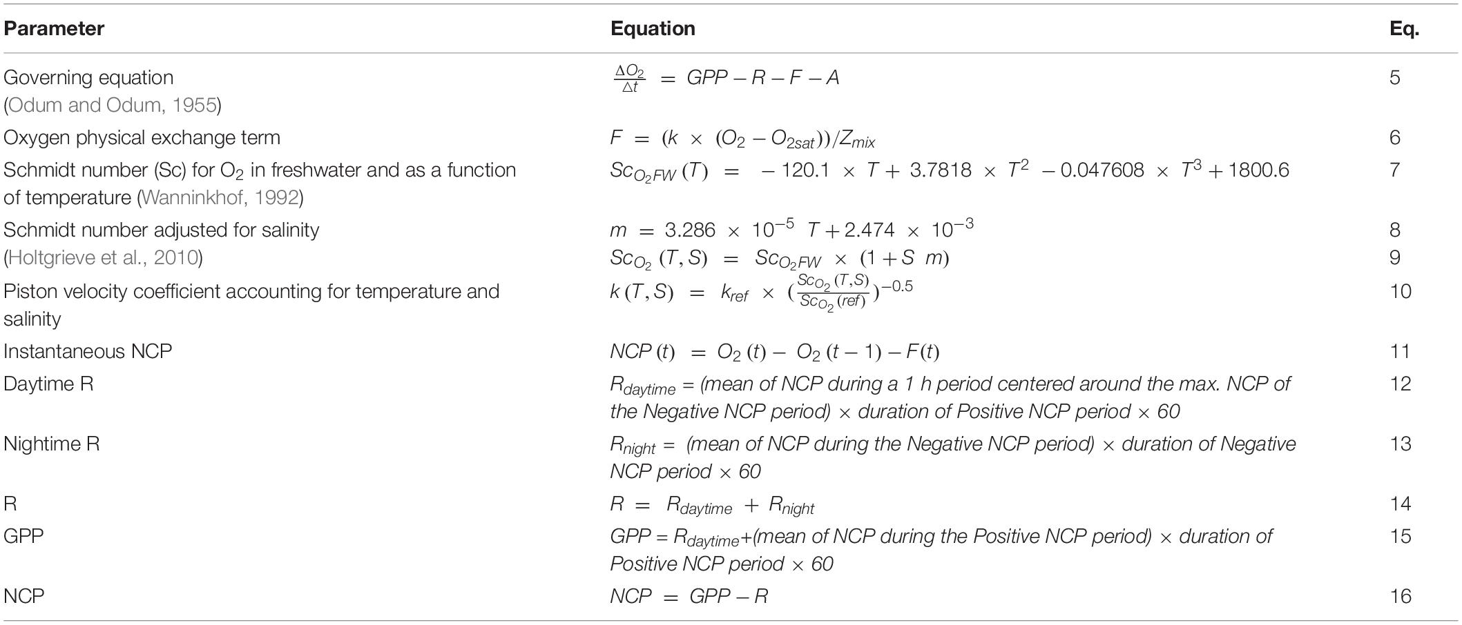
Table 1. Equations used to calculate daily GPP, R, and NCP.

The first step is to calculate the oxygen exchange term F, which is computed as expressed in Eq. 6: where k is the air-water constant, which is also known as the piston velocity coefficient; O₂ and O_2sat are DO concentration and saturation, respectively; and Z_mix is the water column mixing depth. In the case of gently mixed mesocosms, as in the present study, Z_mix can be considered equal to the water column length of the mesocosms. The piston velocity k was adopted from the literature values provided in the study by Soulié et al. (2021). This parameter is determined using water viscosity and O₂ solubility, which are affected by the water temperature and salinity. Therefore, we modeled k every minute as a function of the reference k (k_ref = 0.000156 m min^–1, Alcaraz et al., 2001; Soulié et al., 2021) and of water temperature and salinity, using the following steps. First, the Schmidt number (Sc) for O₂ in freshwater, and as a function of temperature, is given by Eq. 7 (Wanninkhof, 1992), where T is the water temperature. To account for salinity, the coefficient m had be calculated based on the Eq. 8 (Holtgrieve et al., 2010). Finally, the Schmidt number was adjusted for salinity, according to Eq. 9 (Holtgrieve et al., 2010), where S is the salinity and m is the coefficient previously calculated. The piston velocity k was calculated for every 1 min time step using Eq. 10, with Sc_O2(ref) referring to the Schmidt number for the conditions in which k_ref was experimentally measured (16°C, 37.5), which was equal to 675.58.

Second, the instantaneous and the daily metabolic parameters had to be estimated. For each 1 min time step, the instantaneous NCP was calculated according to Eq. 11, in which O₂(t) and O₂(t−1) are the DO concentrations at time t and t-1, respectively; and F(t) is the oxygen exchange term at time t. Daily metabolic parameters could be estimated using the instantaneous NCP for each couple of positive and negative NCP periods. Initially, the respiration during the day, Rdaytime, was calculated according to Eq. 12. In this equation, Rdaytime was expressed in gO₂ m^–3d^–1; the mean instantaneous NCP during a 1-h period (centered on the maximum instantaneous NCP attained during the negative NCP period) was expressed in gO₂ m^–3 min^–1; and the duration of the positive NCP period was expressed in h. Similarly, the respiration during the night, Rnight, could be estimated using Eq. 13.

Rnight was expressed in gO₂ m^–3d^–1, the mean instantaneous NCP during the negative NCP period was expressed in gO₂ m^–3 min^–1 and the duration of the negative NCP period was expressed in h. Thereafter, the daily R (gO₂ m^–3d^–1) was calculated according to Eq. 14 and the daily GPP was estimated using Eq. 15. GPP and Rdaytime were expressed in gO₂ m^–3d^–1, the mean instantaneous NCP during the positive NCP period was in gO₂ m^–3 min^–1, and the duration of the positive NCP period was in h. Finally, daily NCP was calculated as the difference between the daily GPP and daily R (Eq. 16). Due to the lack of a complete DO cycle on the last day of the experiment (d20), NCP, GPP, and R were only estimated from d1 to d19.

Resistance, Resilience, Recovery, and Temporal Stability Estimates

Resistance, resilience, recovery, and temporal stability were calculated for key functions (μ, l, GPP, and R) and for PFTs following the method of Hillebrand et al. (2018) (Table 2). For each day of the HW period, resistance was calculated using the logarithm response ratio (LRR). In addition, the change in resistance during the HW period was calculated as the regression slope of the resistance over time (resistance = slope × time + intercept), following the method of Filiz et al. (2020). A positive change means that the resistance decreases over time for parameters with an average positive resistance, whereas resistance increases over time for parameters with an average negative resistance. Resilience was calculated as the regression slope of the relative LRR function over time during the 10 days of the post-HW period. Recovery was estimated as the LRR on the last day of the experiment. Finally, temporal stability was calculated as the inverse standard deviation of the residuals around resilience. An unpaired t-test was performed to determine if there was a significant difference between resistance over time and benchmark resistance (0) using the R software (version 4.0.1).

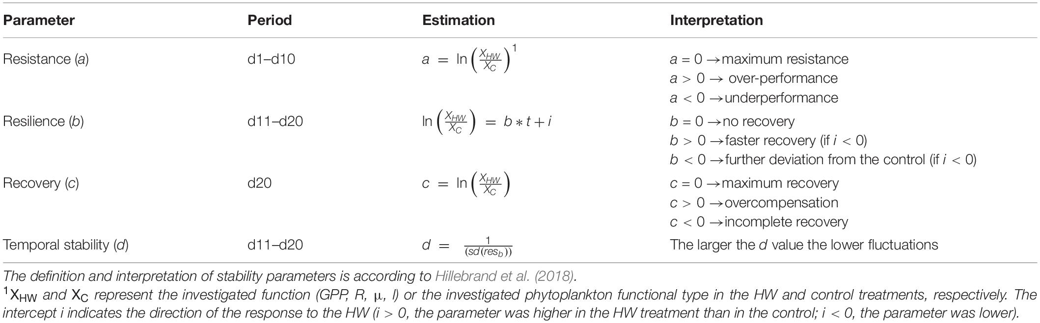
Table 2. Stability parameters estimated in the present study and the experimental period that they are calculated for, as well as their mathematical definition and interpretation.

Statistical Analyses

The difference between treatments was assessed during the 10 days of the HW period (d1–d10), the 10 days of the post-HW period (d11–d19), and during the entire experiment (d1–d19) using repeated-measures analysis of variance, considering treatment assigned as a fixed factor and time as a random factor. Statistical significance was set at p ≤ 0.05. When the assumptions for a parametric test were not met, even if the data were transformed (logarithmic, square root, or exponential transformations), a non-parametric Kruskal–Wallis rank sum test was performed. Principal component analyses (PCA) and ordinary least-square linear relationships were assessed between the LRR of GPP, R, μ, l, PFTs, DLI, temperature, and salinity to assess potential drivers of the system responses (expressed as LRR) to the treatment. Data management and statistical analyses were performed using the R software (version 4.0.1).

Results

Physical and Chemical Conditions

In the control treatment, the water temperature ranged from 17.85 ± 0.02°C (d7) to 20.29 ± 0.01°C (d18). It generally decreased until d7, before increasing and peaking on d13 and d18. In the HW treatment, the water temperature increased by an average of 2.75 ± 0.23°C during the HW period (d1–d10), before returning to the control level during the post-HW period (d11–d19) (Figure 1A). The DLI in the control treatment varied from 7.33 ± 0.85 mol m^–2d^–1 (d1) to 26.32 ± 2.54 mol m^–2d^–1 (d6). It increased from d1 to d4 before being relatively stable and at high values from d6 to d14. The DLI values then decreased until the end of the experiment, with peaks on d14 and d16 (Figure 1B). They were significantly lower in the HW treatment than in the control during both the HW and post-HW periods, by an average of 12 and 11%, respectively (Table 3). The salinity increased during the HW period and remained relatively constant during the post-HW period. In the control, salinity ranged from 38.27 ± 0.17 to 38.73 ± 0.18 (Figure 1C) and was significantly lower in the HW treatment during the HW period by an average of 0.07%, but was significantly higher during the post-HW period by an average of 0.05% (Table 3), compared to the control.

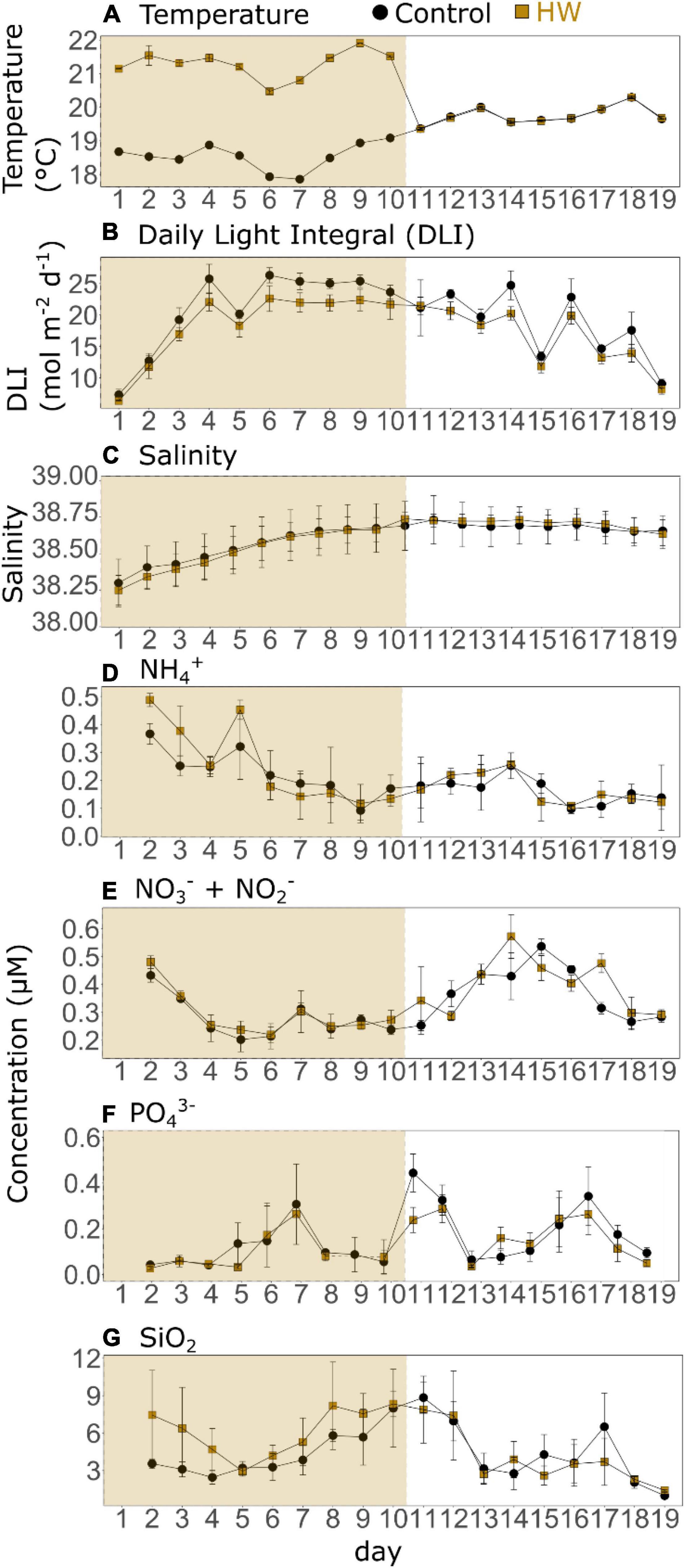
Figure 1. Daily means of water temperature (A), daily light integral (DLI, B), and salinity (C); and daily concentrations of ammonium (NH₄⁺, D), nitrate + nitrite (NO₃^–+NO₂^–, E), orthophosphate (PO₄^3–, F), and silicate (SiO₂, G) in the control (black) and HW (gold) treatments. The gold shaded area represents the HW period during which the +3°C was applied in the HW mesocosms. Error bars represent the standard deviation. Note that the scales of the y-axes are different. Nutrient data were lost on d1 due to a technical problem.

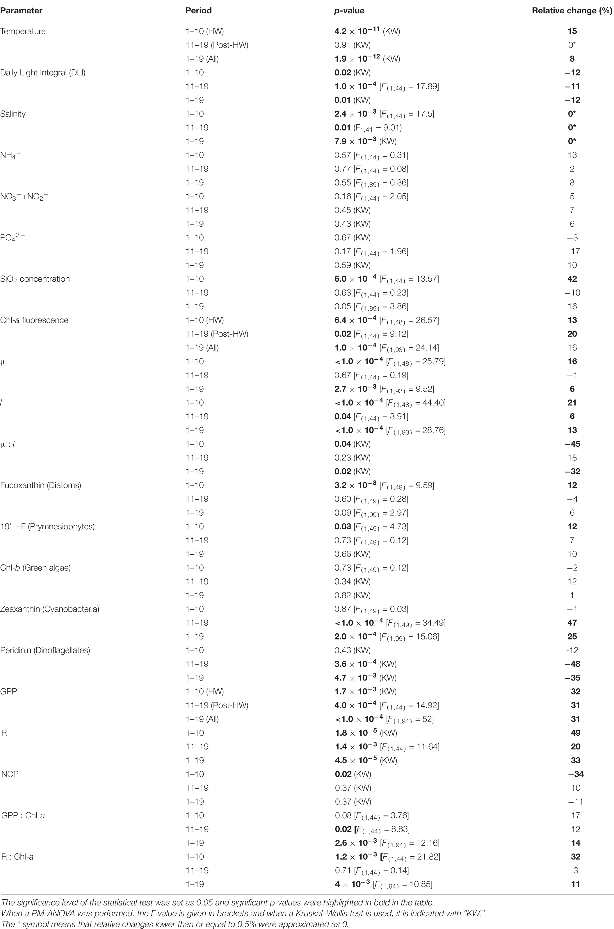
Table 3. Summary table of statistical test results and relative changes between the HW and control treatments in physical, chemical, and biological parameters during the HW period, post-HW period, and during the entire experiment.

The dissolved nutrient concentrations showed varying trends. In the control, the NH₄⁺ concentration ranged from 0.09 ± 0.04 μM (d9) to 0.37 ± 0.04 μM (d1). It generally decreased during the HW period, before remaining relatively constant during the post-HW period (Figure 1D). There was no significant difference between the control and HW treatments in both periods (Table 3). The NO₃^– + NO₂^– concentrations varied from 0.20 ± 0.04 μM (d5) to 0.54 ± 0.03 μM (d15) in the control. It decreased from d2 to d5, but increased until d14 or d15 depending on the treatment, and then decreased again until the end of the experiment (Figure 1E). Similar to the NH₄⁺ concentrations, there was no significant difference in NO₃^– and NO₂^– concentrations between the control and HW treatments during both periods (Table 3). In the control, the PO₄^3– concentration ranged from 0.04 ± 0.01 μM to 0.44 ± 0.02 μM, which peaked three times during the experiment (d7, d11, d17) (Figure 1F). As for N-nutrients, there was no significant difference between treatments in the HW and post-HW periods (Table 3). Finally, in the control treatment, the SiO₂ concentration ranged from 0.98 ± 0.27 μM (d1) to 8.84 ± 1.22 μM (d11), and it increased from d4 to d11, and later it decreased until the end of the experiment, except for a peak on d17 (Figure 1G). In contrast to the other nutrient concentrations, SiO₂ concentrations were significantly higher during the HW period by an average of 42%, but no significant differences between treatments were found in the post-HW period (Table 3).

Phytoplankton Community: Chlorophyll-a Fluorescence, μ, l, and Phytoplankton Functional Types

The chl-a fluorescence dynamics indicated that the experiment started during a phytoplankton bloom. This was evidenced by the concentrations, which increased from d1 to d2 reaching 4.04 ± 0.51 μg L^–1 in the control treatment, decreased until d13 with the lowest value being 1.21 ± 0.13 μg L^–1, and then slightly increased again until the end of the experiment (Figure 2A). The HW treatment had similar dynamics, peaking on d2 before decreasing in both the HW and post-HW periods. Concentrations were significantly higher in the HW treatment than in the control, by an average of 13 and 20%, respectively (Table 3). In the control, μ varied from 0.26 ± 0.03 d^–1 (d5) to 0.97 ± 0.04 d^–1 (d19). During the HW period, it was relatively constant and generally higher than 0.3 d^–1, except on d5 (0.26 ± 0.03 d^–1). During the post-HW period, there were more fluctuations, with peaks on d13, d15, d17, and d19 (Figure 2B). In the HW treatment, μ was significantly higher than in the control treatment by an average of 16% during the HW period, but no significant effect was found in the post-HW period (Table 3). In the control, l ranged from 0.28 ± 0.03 d^–1 (d5) to 1.27 ± 0.04 d^–1 (d19); it increased from d5 to d9 and from d12 to d19 (Figure 2C). Similar to μ, l was significantly higher in the HW treatment than in the control during the HW period, by an average of 21%; however, different from μ, l remained significantly higher in the HW treatment than in the control during the post-HW period, by an average of 6% (Table 3). In the control treatment, as μ was generally lower than l, the μ:l ratio was negative 16 days out of the 19 (Figure 2D). The ratio was significantly lower in the HW treatment than in the control during the HW period, by an average of 45%, but it was not significantly changed during the post-HW period (Table 3).

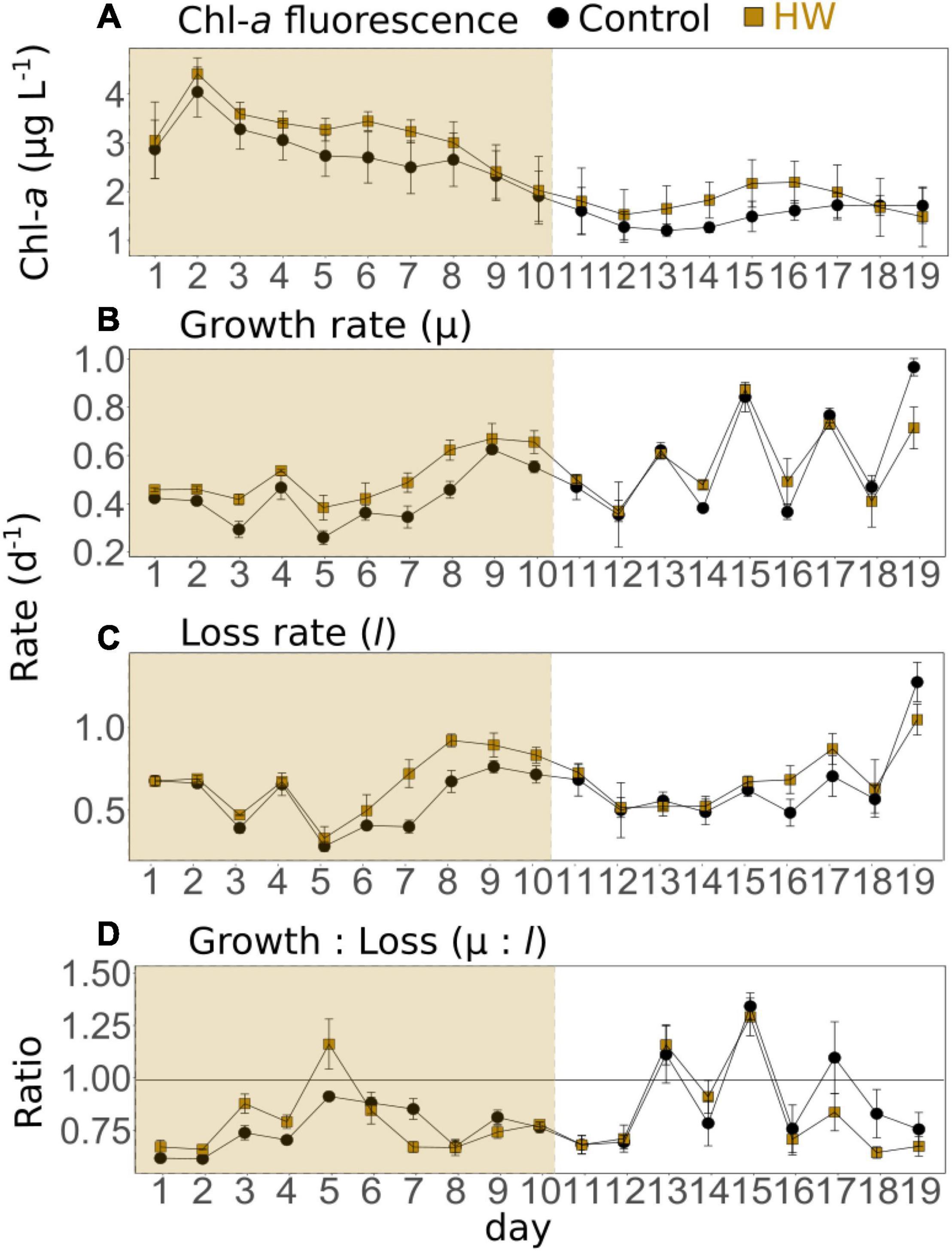
Figure 2. Daily means of phytoplankton chlorophyll-a fluorescence (corrected for NPQ, A), μ (B), l (C), and μ:l (D) in the control (black) and HW (gold) treatments. The gold shaded area represents the HW period during which the +3°C was applied in the HW mesocosms. Error bars represent the standard deviation.

In the control treatment, the main phytoplankton taxonomic pigments were the fucoxanthin (associated with diatoms) and the 19′-HF (associated with prymnesiophytes), with average concentrations of 1.17 ± 0.17 and 1.27 ± 0.21 μg L^–1, respectively. Peridinin (associated with dinoflagellates), chl-b (associated with green algae), and zeaxanthin (associated with cyanobacteria) were present at lower concentrations. The fucoxanthin, 19′-HF, and chl-b concentrations followed a similar temporal trend (Figures 3A,C,D). They increased at the beginning of the experiment, decreased until d12 or d13 depending on the pigment, and then increased again at the end of the experiment. However, while fucoxanthin and chl-b concentrations decreased rapidly after attaining a peak on d3, and 19′-HF concentration remained high until d10. At the beginning of the experiment, the peridinin concentration was extremely low (below the detection limit), then it generally increased until d14 with peaks on d9, d11, and d14. The peridinin concentration then decreased on d15 and remained relatively constant until the end of the experiment (Figure 3B). The zeaxanthin concentration remained relatively constant during the entire experiment, peaking on d4, d7, and d15 and reached its minimum on d9 (Figure 3E). During the HW period, a significant increase was found in the HW treatment for fucoxanthin and 19′-HF concentrations, both by an average of 12% (Table 3). During the post-HW period, the zeaxanthin concentrations were significantly higher in the HW treatment by an average of 47%, whereas the peridinin concentrations were significantly lower by an average of 48% (Table 3). No other significant differences between the two treatments were observed.

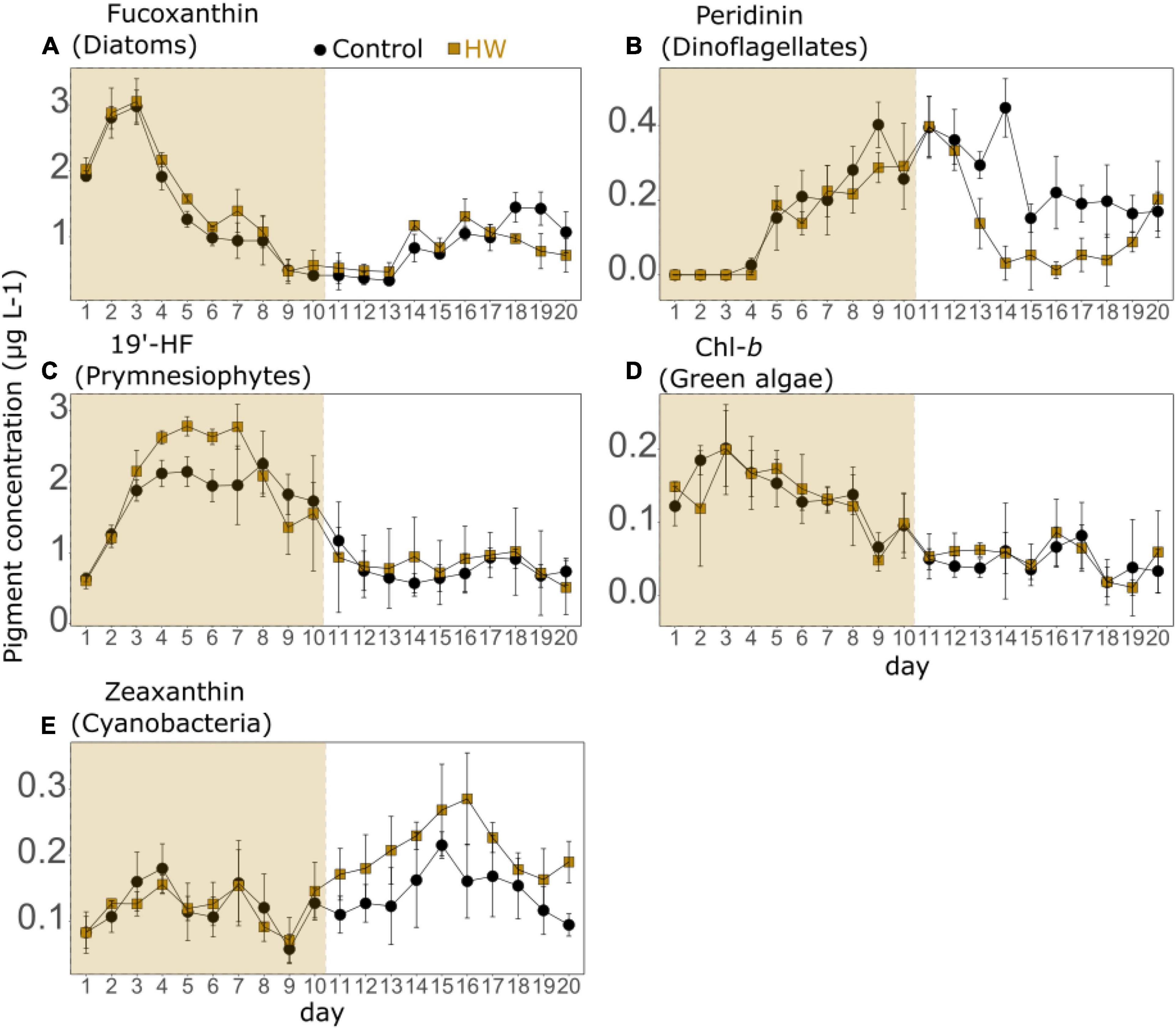
Figure 3. Phytoplankton functional types (PFTs) assessed as daily mean concentrations of fucoxanthin (A), peridinin (B), 19′-hexanoyloxyfucoxanthin (19′-HF, C), chlorophyll-b (Chl-b, D), and zeaxanthin (E) in the control (black) and HW (gold) treatments. The gold shaded area represents the HW period during which the +3°C was applied in the HW mesocosms. Error bars represent the standard deviation. Note that the scales of the y-axes are different.

Plankton Community Metabolism: Gross Primary Production, Respiration, and Net Community Production

In the control treatment, the GPP ranged from 0.27 ± 0.01 (d3) to 0.95 ± 0.08 gO₂ m^–3d^–1 (d16). It peaked on d8 and d16 (Figure 4A). During both the HW and post-HW periods, it was significantly greater in the HW treatment compared to the control, by an average of 32 and 31%, respectively (Table 3). The highest difference was observed on d15, with the GPP being 94% higher in the HW treatment. On the last 2 days of the post-HW period (d18 and d19), GPP values decreased and were similar to those of the control treatment. R varied from 0.29 ± 0.01 gO₂ m^–3d^–1 (d3) to 0.81 ± 0.09 gO₂ m^–3d^–1 (d18). It remained relatively constant during the entire experiment, except between d11 and d13 and between d15 and d18 when it increased (Figure 4B). Similar to the GPP, R increased significantly in the HW treatment during the HW period by an average of 49%, compared to the control (Table 3). In addition, R was significantly higher in the HW treatment during the post-HW period, by an average of 20%, but returned to the control level on d19. The largest difference between treatments was found on d15 (95%). As a consequence, in the control treatment, the NCP was positive on 10 days out of 19 days; it ranged from −0.19 ± 0.06 (d18) to 0.20 ± 0.03 gO₂ m^–3d^–1 (d8). The mean NCP (3.2 × 10^–3 ± 0.03 gO₂ m^–3d^–1) indicated a globally autotrophic system (Figure 4C). In the HW treatment, the NCP was positive on 7 days out of 19 days, with a mean value of 6.1 × 10^–3 ± 0.10 gO₂ m^–3d^–1. During the HW period, the NCP was significantly reduced in the HW treatment, compared to the control, by an average of 157% (Table 3). In the post-HW period, however, no statistically significant differences were found between the two treatments. GPP and R were also normalized by chl-a fluorescence (Figures 4D,E). During the HW period, the GPP:chl-a ratio was not significantly different between treatments, whereas R:chl-a was significantly higher in the HW treatment by an average of 32% (Table 3). Conversely, during the post-HW period, GPP:chl-a was significantly higher in the HW treatment by an average of 12%, whereas no significant differences were found between treatments for R:chl-a.

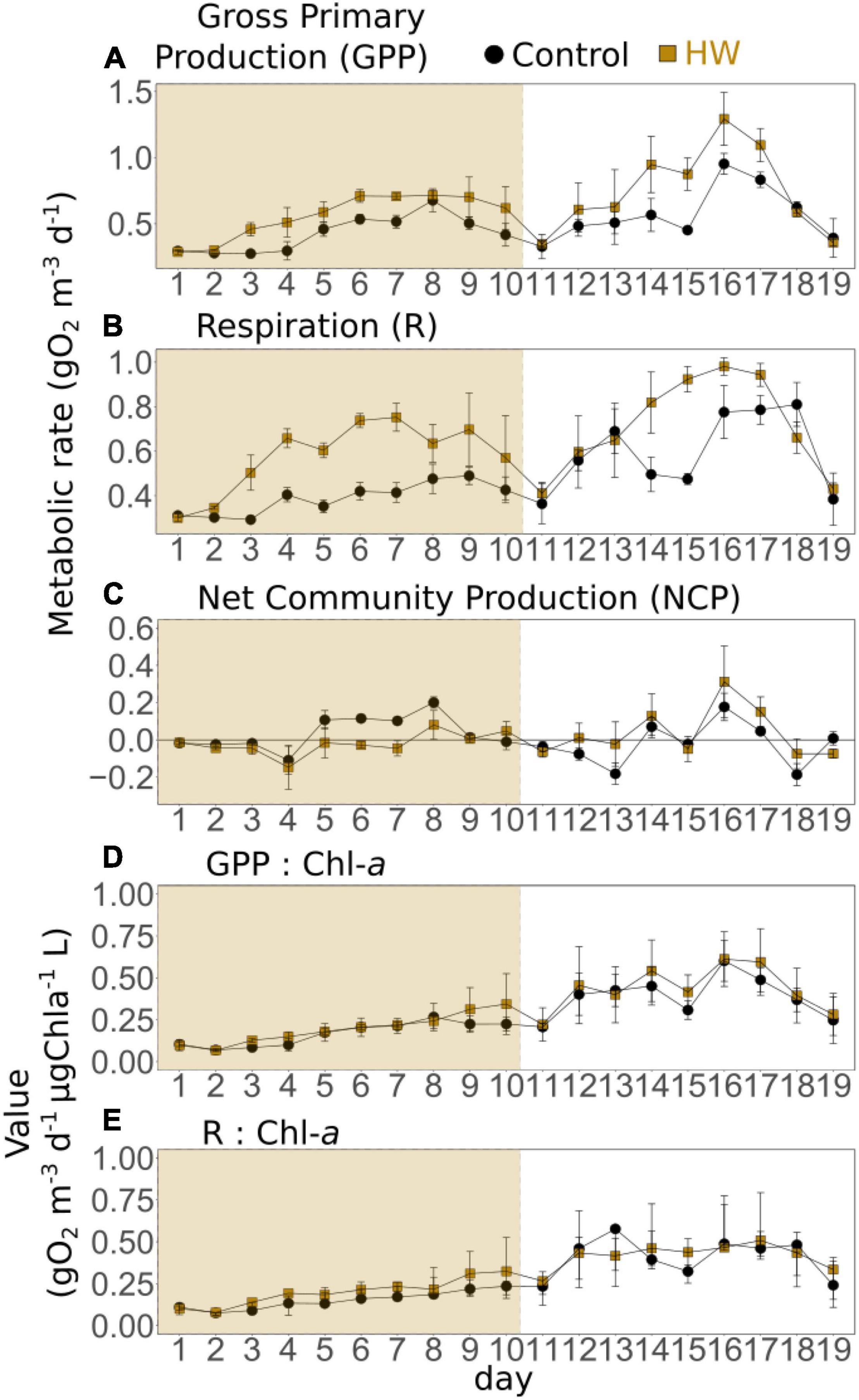
Figure 4. Daily means of gross primary production (GPP, A), respiration (R, B), net community production (NCP, C), GPP normalized by chlorophyll-a fluorescence (D), and R normalized by chlorophyll-a fluorescence (E) in the control (black) and HW (gold) treatments. The gold shaded area represents the HW period during which the +3°C was applied in the HW mesocosms. Error bars represent the standard deviation.

Relationships Between Plankton Metabolism, Pigment, and Environmental Variables

Principal component analyses were performed to highlight the potential correlations between plankton metabolic rates, PFTs, and the LRR of the environmental variables during the HW and post-HW periods (Figure 5). PCA enabled the projection of variables in a multidimensional space and showed the relationships between the LRR of metabolic and environmental variables (Figures 5A,B) and between the LRR of metabolic variables and PFTs (Figures 5C,D). Moreover, ordinary least squares linear relationships between the LRR of metabolic variables, PFTs, and environmental variables were assessed to refine the relationship between specific variables. Only relationships that were found to be significant (p < 0.05) during at least one of the tested periods are shown in Table 4.

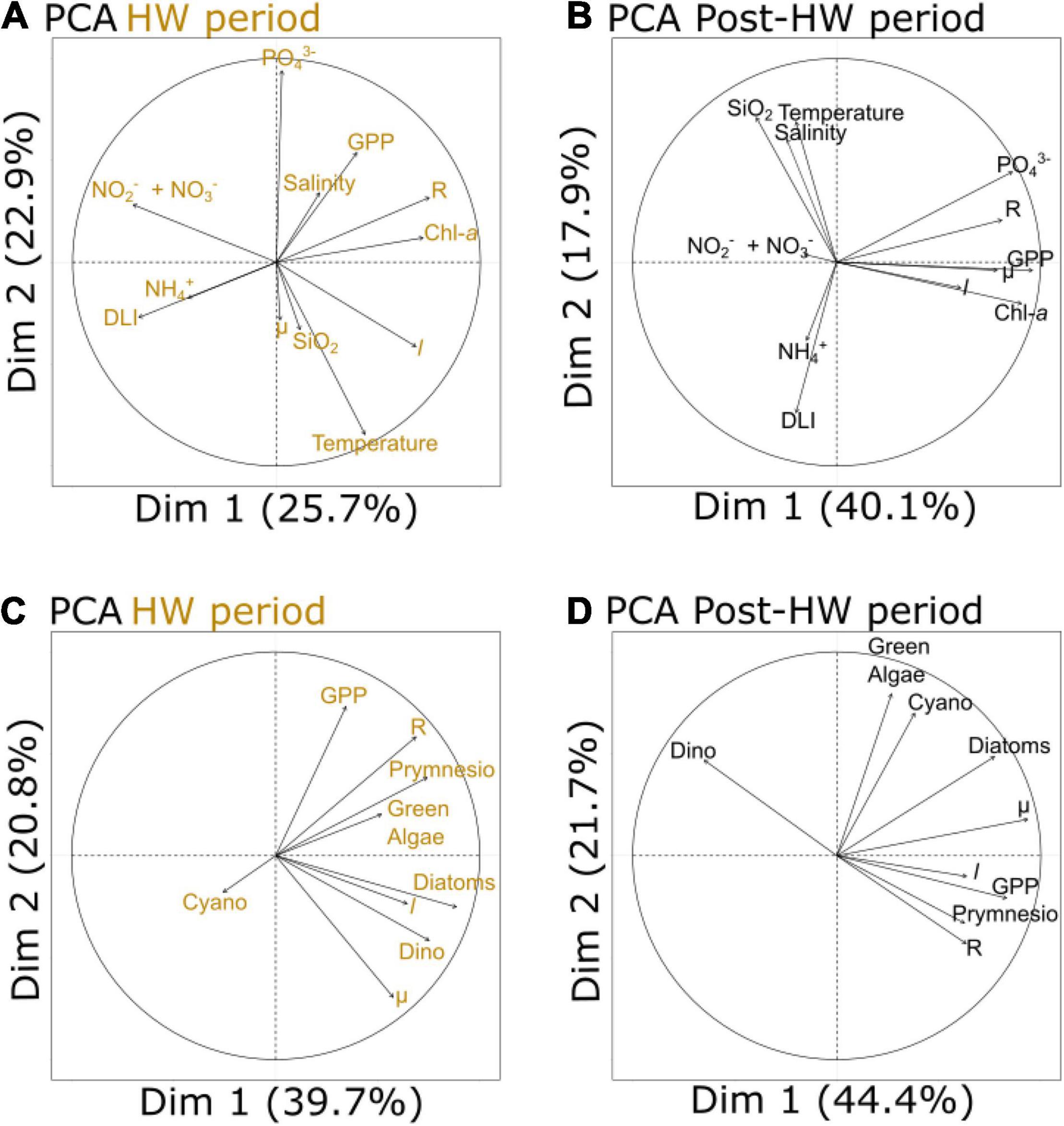
Figure 5. Principal component analyses (PCA) of the log response ratio (LRR) of metabolic and environmental variables during the HW period (A) and the post-HW period (B), as well as PCA of the LRR of metabolic variables and PFTs during the HW period (C) and the post-HW period (D). When variables are close to each other, they are positively correlated. When they are opposed, they are negatively correlated. When they are orthogonally located, they are not correlated. When variables are close to the center, they are not well represented by the analysis.

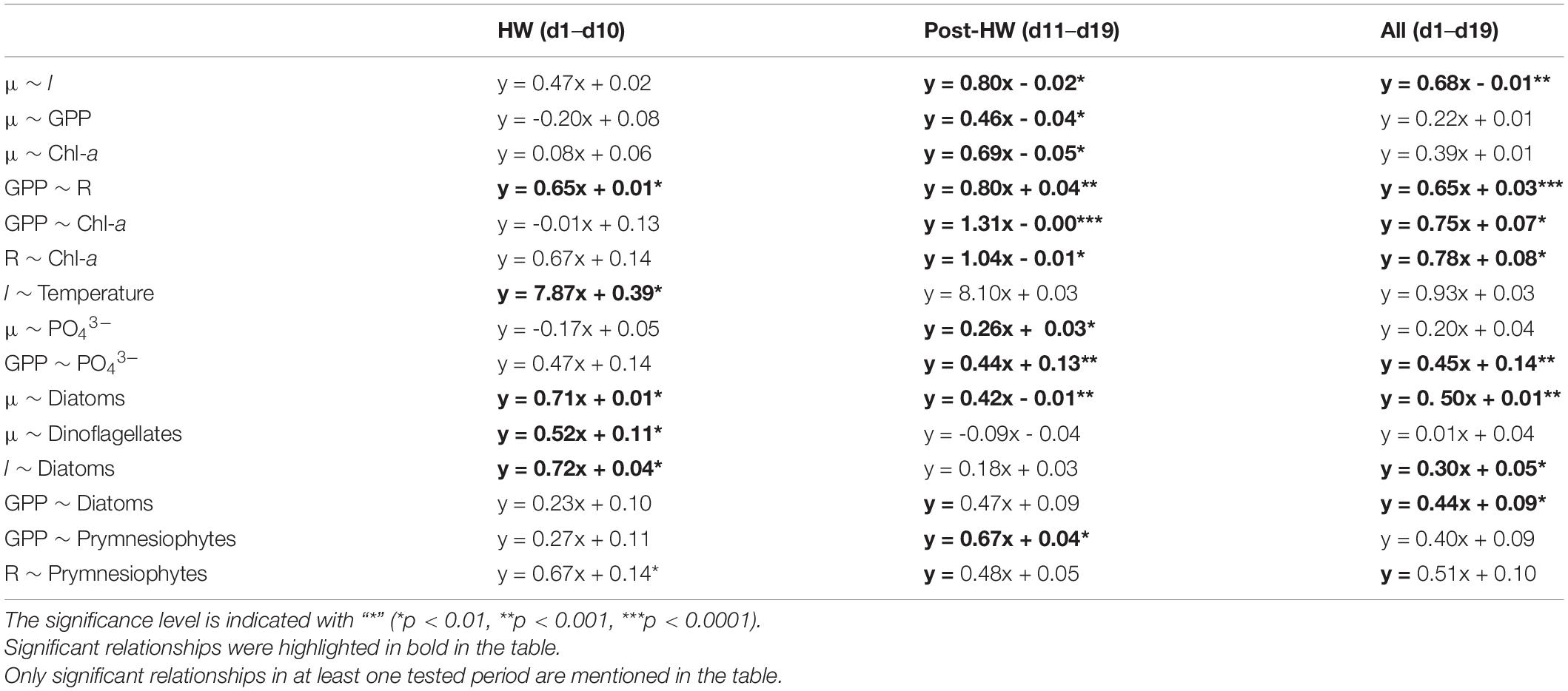
Table 4. Ordinary least squares linear relationships between plankton community metabolism, PFTs, and environmental variables.

For both periods, GPP, R, and chl-a fluorescence were clustered near the first PCA axis (Figures 5A,B). Salinity was part of this group during the HW period while μ, l, and PO₄^3– concentrations were part of it during the post-HW period (Figure 5B). During the HW period, this group was opposed to DLI and concentrations of NO₃^–, NO₂^–, and NH₄⁺, suggesting a negative relationship between them. In line with these results, a significantly positive linear relationship was found between GPP and R, and between l and temperature during the HW period (Table 4). During the post-HW period, significant relationships were found between μ and l, chl-a fluorescence and PO₄^3– concentration, GPP and R, chl-a fluorescence and PO₄^3– concentration, and between R and chl-a fluorescence. During the HW period, μ appeared to be close to dinoflagellates while l was close to both dinoflagellates and diatoms (Figure 5C). Meanwhile, R was close to the prymnesiophytes and green algae. During the post-HW period, GPP, R, and l were part of a group alongside prymnesiophytes and opposed to dinoflagellates (Figure 5D). A significant linear relationship was found between μ and diatoms in both periods and between μ and dinoflagellates during the HW period (Table 4). Diatoms were also positively correlated with l during the HW period. In addition, GPP, diatoms, and prymnesiophytes were found to be positively related while considering the entire experiment and the post-HW period, respectively. Finally, R and prymnesiophytes were also linearly related, but only during the HW period (Table 4).

Stability Parameters

The resistance over the 10-days HW period was significantly different from the benchmark resistance for all studied functions (μ, l, GPP, and R) and for diatoms, but not for all the other PFTs (Figure 6). The change in resistance during the HW period was negative for all investigated parameters, except for prymnesiophytes, indicating that their resistance increased over time for parameters with a positive average resistance (μ, l, GPP, R, diatoms, cyanobacteria), but decreased over time for parameters with a negative average resistance (green algae, dinoflagellates) (Figure 6).

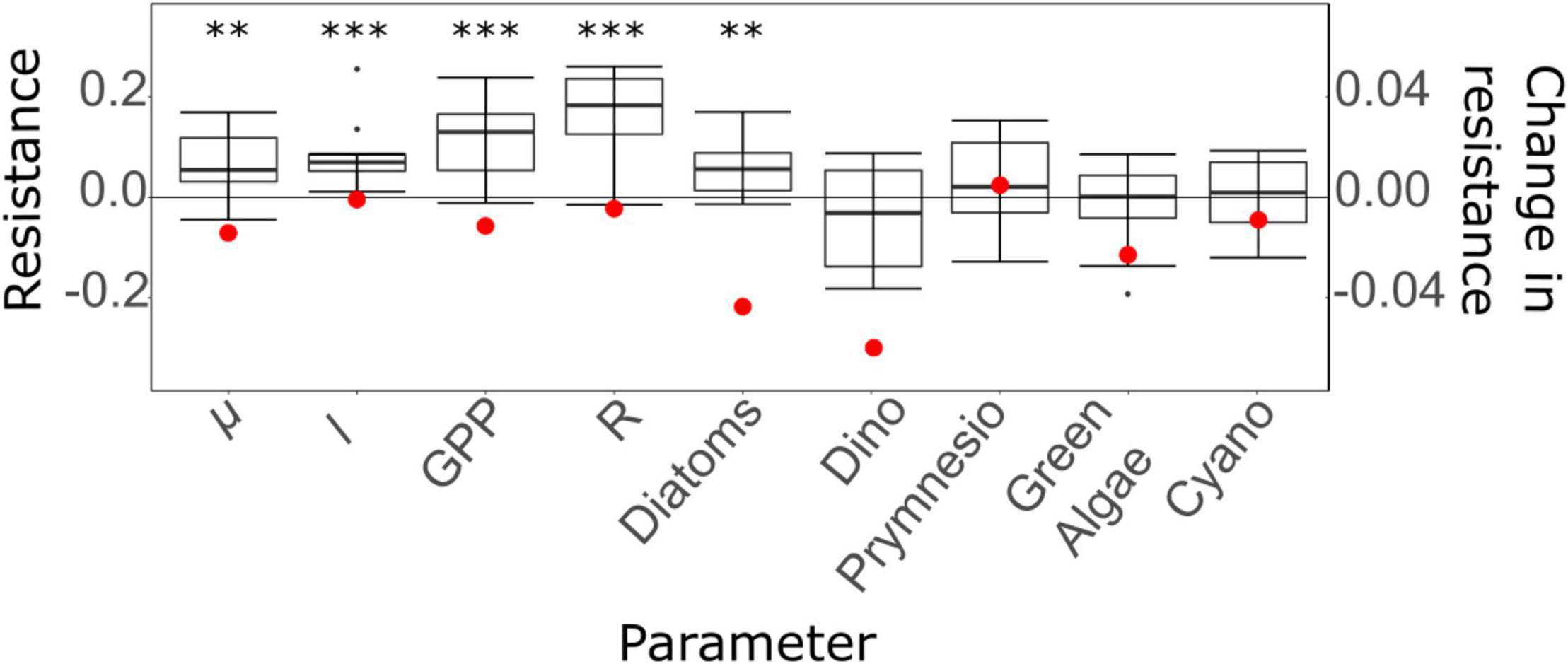
Figure 6. Boxplot of resistance over time and change in resistance over time (red dots) for planktonic processes (μ, l, GPP, R) and phytoplankton functional types (Dino: dinoflagellates, Prymnesio: prymnesiophytes, Cyano: cyanobacteria). The results of an unpaired t-test testing the difference between resistance and benchmark value (0) for each parameter are presented over the boxplots when a significant p-value was found (^**, p < 0.01; ^***, p < 0.001).

The average resistance over the HW period was closer to the benchmark resistance for μ and l compared to GPP and R (Table 5), which indicates a better resistance for μ and l than for GPP and R. Among all the tested functions, the system was shown to be the most resistant in terms of μ and least resistant in terms of R. In addition, all resilience values were close to 0 (the benchmark resilience) and negative, indicating that all functions continued to deviate from the control during the post-HW period. The functions that had the worst and best recoveries were μ and GPP, respectively. Finally, the largest temporal stability was found for μ and l, whereas GPP and R exhibited lower temporal stability levels (Table 5). Among PFTs, the highest resistance was found for cyanobacteria, followed by prymnesiophytes and green algae, whereas diatoms displayed the lowest resistance (Table 5). As for the functions, all resilience values, except for those of prymnesiophytes, were negative and close to the benchmark, indicating a low resilience and a further deviation from the control after the heatwave. Furthermore, green algae and prymnesiophytes displayed the worst and best recoveries, respectively, and diatoms and prymnesiophytes had the highest levels of temporal stability, whereas dinoflagellates had the lowest (Table 5).

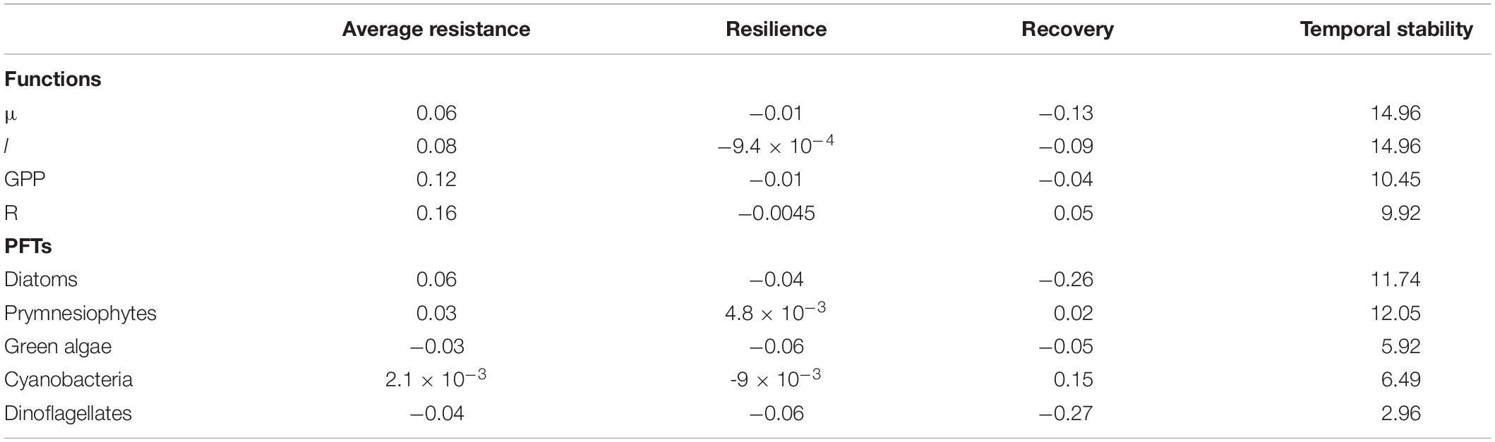
Table 5. Average resistance, resilience, recovery, and temporal stability in terms of μ, l, GPP, R, and PFTs.

Discussion

The Heatwave Enhanced Functional Processes and Changed Phytoplankton Community Structure

The aim of the present study was to assess the effects of a simulated heatwave on the plankton community in a coastal Mediterranean lagoon during the late spring/early summer; the primary focus was on phytoplankton growth and loss rates, functional types, and plankton community metabolism. During the HW period, phytoplankton μ, l, GPP, and R increased by an average of 16, 21, 32, and 49%, respectively, in the HW treatment compared to the control.

These positive effects of the heatwave on μ and GPP are congruent with the theoretical predictions of the metabolic theory of ecology (MTE, Brown et al., 2004), with in situ observations (López-Urrutia et al., 2006; Regaudie-de-Gioux and Duarte, 2012), and with results from experiments (Eppley, 1972; Vázquez-Domínguez et al., 2007; Panigrahi et al., 2013). In the present study, μ and diatom responses to the treatment were significantly related, meaning that the observed rise in μ was certainly due to a positive effect on diatoms. This positive effect on diatoms was consistent with studies reporting higher diatom abundances under warmer conditions (Zhu et al., 2017; Sett et al., 2018; Hyun et al., 2020); this may be due to the high SiO₂ concentrations found in both treatments at the beginning of the experiment. Moreover, the Si:N and Si:P ratios appeared to be unusually high for the system at this time of the year (Liess et al., 2015; Trombetta et al., 2019), which probably favored diatoms over other phytoplankton groups. Thus, the higher SiO₂ concentrations found in the HW treatment might have resulted in the higher diatom-associated pigment concentration in the HW treatment. This is consistent with the fact that nutrient availability often overrides temperature in phytoplankton responses to heatwaves (Marañón et al., 2014; Hayashida et al., 2020; Sen Gupta et al., 2020; Domingues et al., 2021). Finally, in the present study, when normalized by the chl-a fluorescence, the GPP was not significantly different between treatments, indicating that the positive effect of the heatwave on GPP was primarily due to the increase in phytoplankton biomass. This suggests that it is phytoplankton biomass dynamics, and therefore μ and l, that drive the GPP response to heatwaves.

Heating increased l during the HW period, suggesting a boost in grazing and viral lysis. These two processes have been reported to be enhanced by warming (Rose and Caron, 2007; Rose et al., 2009; Aberle et al., 2012; Lara et al., 2013). Consistent with this observation, the positive effect of the treatment on l was positively related to the temperature difference between treatments. Notably, l increased only several days after the start of the heatwave, whereas μ increased at the beginning of the heatwave. This mismatch in the timing of the responses of μ and l indicates why the phytoplankton biomass was higher in the HW treatment than in the control. However, during the second part of the heatwave, l increased more than μ, and the μ:l ratio was negatively affected by the heatwave. This is in line with a meta-analysis of the μ to grazing ratio dataset estimated in temperate coastal areas that reported a negative effect of temperature on this ratio (Cabrerizo and Marañón, 2021). The μ:l ratio is a major factor controlling the fate of newly produced organic matter in the ocean and has important implications for element cycling. Our study implies that future heatwaves could alter the coupling between phytoplankton and their grazers, with major impacts on the structure of the microbial food web (Calbet and Landry, 2004).

Similarly, community R increased more than GPP during the HW period, supporting general observations that are in line with theoretical predictions from the MTE, which reported a greater positive effect of warmer conditions on R than on GPP because of the higher activation energy for R (López-Urrutia et al., 2006; Yvon-Durocher et al., 2010; Regaudie-de-Gioux and Duarte, 2012; Vaquer-Sunyer and Duarte, 2013). In contrast to GPP, when normalized by chl-a fluorescence, R remained significantly higher in the HW treatment than the control, indicating that the positive effect of the heatwave on R was because of processes other than just the increase in phytoplankton biomass. This positive effect on R:chl-a probably depicts a positive response of bacterial respiration, which is normally the major contributor to community R in coastal waters (Robinson, 2008). Nevertheless, the strong positive relationship found between the heatwave effects on GPP and R suggests that bacterial R is partly dependent on autotrophic production as a carbon source, as suggested by studies demonstrating the importance of phytoplankton exudates for bacterial metabolism (del Giorgio and Cole, 1998). As a consequence of the greater increase in R than in GPP during the HW period, the NCP was reduced toward global heterotrophy. Thus, the present study indicates that moderate heatwaves could shift coastal Mediterranean lagoons from oxygen producers to oxygen sinks. Combined with the physical deoxygenation due to global warming and higher water temperatures, heatwaves could lead to hypoxia or anoxia events, which are known to have dramatic consequences for coastal Mediterranean lagoon ecosystems (Viaroli et al., 2010).

All the investigated processes showed low resistance during the HW period as evidenced by their higher values in the HW treatment than in the control. However, their resistance increased as the heatwave progressed. This suggests that the plankton community became acclimated to the disturbance. As the duration of heatwaves have increased during the past decade in the Mediterranean area (Kuglitsch et al., 2010), the effect of heatwaves on planktonic processes might be mitigated by this acclimation process. All PFTs, except diatoms, were found to be resistant to heatwaves, suggesting that heatwave-induced changes in phytoplankton community composition take more time to occur than changes in planktonic processes.

Most Plankton Processes Showed a Low Resilience That Was Associated With Important Changes in the Phytoplankton Community Structure

The recovery trend of the plankton community processes, assessed during the post-HW period, revealed the low resilience of GPP, R, and l, as they were significantly higher in the HW treatment than in the control, by 6, 31, and 20%, respectively. However, μ recovered rapidly from the heatwave, as it was not significantly higher in the HW treatment than in the control, in contrast to what was observed during the HW period.

Phytoplankton l was still higher in the HF treatment than in the control during the post-HW period, but to a lesser extent than that during the HW period. This suggests that l partly underwent a recovery process. However, as the difference persisted, it indicated that the heatwave probably accelerated zooplankton development and metabolism during the HW period (Hart and McLaren, 1978; Vidussi et al., 2011; Weydmann et al., 2017), which resulted in greater zooplankton grazing pressure that persisted during the post-HW period. This explains the higher l found in the HF treatment during the post-HW period. Nonetheless, the μ:l ratio was not significantly different between treatments during the post-HW period, indicating that the imbalance toward l found during the HW period did not persist during the post-HW period. This suggests that the heatwave-induced decoupling between phytoplankton and their predators does not persist in the long term.

In contrast to l, GPP, and R further deviated from the control during the post-HW period, as they were higher in the HW treatment than in the control. This phenomenon is indicated by their poor resilience values. This result is congruent with what is typically observed for shallow lake plankton communities, as the positive effect of a simulated heatwave on GPP and R persisted several days after the end of the heatwave, regardless of the nutrient status or initial temperature (Jeppesen et al., 2021). Notably, when normalized by chl-a fluorescence, R was not significantly different between treatments, whereas GPP remained significantly higher in the HW treatment. This means that the higher R is most probably due to higher phytoplankton biomass while the higher GPP could also depict a physiological response of the phytoplankton. This result is further supported by the fact that R was positively related to chl-a fluorescence and μ during the post-HW period, which is in contrast to that reported during the HW period. This could indicate that bacterial R relied mainly on phytoplankton production and that phytoplanktonic R might have accounted for a significant part of the total community R during the post-HW period, as expected during late spring and summer (Regaudie-de-Gioux and Duarte, 2012). Nonetheless, both the responses of GPP and μ to the treatment were related to PO₄^3– concentrations during the post-HW period, indicating that PO₄^3– availability might have regulated phytoplankton processes. This was not surprising, as it is known that Thau Lagoon phytoplankton can be controlled by phosphorus (Gowen et al., 2015; Derolez et al., 2020).

During the post-HW period, NCP shifted toward autotrophy in the HW treatment, as GPP had increased more than R, in contrast to what was observed during the HW period. This contradicts the theoretical predictions of the MTE, but might be explained by indirect effects that reduce the magnitude of R. Indeed, this could be explained by a trophic cascade through a positive effect of warming on the predators of bacteria (e.g., heterotrophic flagellates) during the HW period, resulting in increased grazing on bacteria that persisted throughout the post-HW period. In this way, bacteria and R were reduced as shown in a previous study in the same lagoon during the same season (Vidussi et al., 2011). The GPP and R recovered well at the end of the post-HW period, as they returned to the control treatment level. This recovery is certainly due to the fact that the phytoplankton biomass returned to the control level possibly owing to nutrient limitation, as nutrient concentrations tended to decrease in both treatments at the end of the experiment. Nevertheless, this indicates that HW could induce significant but reversible changes in plankton metabolism in Mediterranean coastal waters.

In addition to the remarkable changes reported on planktonic processes, the phytoplankton community structure was also significantly affected during the post-HW period as cyanobacteria seemed to have been favored in the HW treatment at the expense of dinoflagellates. Hence, cyanobacteria might have been the major contributor to the increase in phytoplankton biomass during the post-HW period. This is in contrast to what was observed during the HW period when it was certainly diatoms and prymnesiophytes that contributed to the increase in phytoplankton biomass. Studies have reported that cyanobacteria are often favored under high-temperature conditions in the Mediterranean (Agawin et al., 1998; Maugendre et al., 2015; Courboulès et al., 2021). However, in the present study, they increased only during the post-HW period, suggesting a potential competition with other phytoplankton groups for nutrients, which caused this delay. As explained earlier, diatoms might have been favored by the unusually high Si:N and Si:P ratios, which could have resulted because of the intense competitive pressure between cyanobacteria and diatoms. Moreover, SiO₂ concentration is known to be a key regulator of competition between the two groups (Horn and Uhlmann, 1995). Consequently, when the competitive pressure of diatoms decreased during the post-HW period, cyanobacteria were potentially released from intense competition for nutrients and began to grow in numbers. This increase was also concomitant with a strong decrease in dinoflagellates, suggesting that dinoflagellates were outcompeted by cyanobacteria during the post-HW period in the HW treatment, possibly due to a cyanobacterial allelopathic mechanism inhibiting dinoflagellate photosynthetic activity, as observed in cyanobacterial blooms (Sukenik et al., 2002). As dinoflagellates and cyanobacteria have different chemical requirements for their specific processes and play different roles within the food web, this change suggests that heatwaves could deeply alter both biogeochemical cycles and interactions among organisms. Finally, this might also explain the poor stability of planktonic processes during the post-HW period as the lack of compositional recovery often results in low functional resilience and recovery levels (Hillebrand and Kunze, 2020).

Conclusion and Outlooks

The novel design of the present study allowed us to highlight significant changes in the metabolism of a Mediterranean coastal lagoon plankton community in response to a simulated moderate heatwave during the late spring/early summer. We were also able to assess the resistance and recovery trajectory of the community. During the heatwave, phytoplankton biomass, growth, losses, and oxygen metabolic parameters were all amplified by the simulated heatwave. This positive effect persisted several days after the offset of the heatwave, indicating poor resilience of all the tested functions. Nevertheless, GPP and R recovered well at the end of the experiment, indicating that the effects of heatwaves on plankton metabolism could be reversible. In addition, the simulated heatwave induced notable changes in the structure of the phytoplankton functional types, suggesting that diatoms, prymnesiophytes, and cyanobacteria could be potential winners under more frequent heatwaves occurring in the late spring/early summer period in the lagoon, while dinoflagellates could be the main losers.

The use of in situ mesocosm experiments and high-frequency sensors enabled us to elucidate the effects of heatwaves on coastal plankton community function, which is necessary to refine model predictions for the future of aquatic ecosystems. The results reported in the present study were obtained during one mesocosm experiment at one location during one season; thus, their generalization to other areas or seasons must be done with this awareness. Nevertheless, the present work contributes to a broader understanding of marine heatwaves and their potential impacts on coastal Mediterranean plankton assemblages.

Data Availability Statement

The raw data supporting the conclusions of this article will be made available by the authors, without undue reservation.

Author Contributions

BM and FV conceived and designed the study, and performed the mesocosm experiment. BM, FV, and SM managed the experiment. TS and SM calibrated all sensors used in this study. All authors participated in the daily sampling in the mesocosms. TS and FV performed phytoplankton pigment analyses using HPLC. TS processed the sensor data, made the related analyses, and wrote the original draft of the manuscript with inputs from all authors.

Funding

The present work, plus a part of the grant of TS, was funded under the AQUACOSM project, which have received funding from the European Union’s Horizon 2020 Research and Innovation Program (H2020/2017–2020) under grant agreement n°731065.

Conflict of Interest

The authors declare that the research was conducted in the absence of any commercial or financial relationships that could be construed as a potential conflict of interest.

Publisher’s Note

All claims expressed in this article are solely those of the authors and do not necessarily represent those of their affiliated organizations, or those of the publisher, the editors and the reviewers. Any product that may be evaluated in this article, or claim that may be made by its manufacturer, is not guaranteed or endorsed by the publisher.

Acknowledgments

We would like to thank Rémi Valdès, Solenn Soriano, Kevin Mestre, Camille Suarez-Bazille, and David Parin from MEDIMEER for their valuable help with the mesocosm setup, daily sampling, dissolved nutrient analyses, and sensor setup during the experiment. We would also like to thank Emilie Eveque, Jean-François Thevenot, and many other partners from the AQUACOSM Transnational Access for their assistance with daily sampling.

References

Aberle, N., Bauer, B., Lewandowska, A., Gaedke, U., and Sommer, U. (2012). Warming induces shifts in microzooplankton phenology and reduces time-lags between phytoplankton and protozoan production. Mar. Biol. 159, 2441–2453. doi: 10.1007/s00227-012-1947-0
Agawin, N. S. R., Duarte, C. M., and Agusti, S. (1998). Growth and abundance of Synechococcus sp. in a Mediterranean Bay: seasonality and relationship with temperature. Mar. Ecol. Prog. Ser. 170, 45–53. doi: 10.3354/meps170045
Alcaraz, M., Marrasé, C., Peters, F., Arin, L., and Malits, A. (2001). Seawater–atmosphere O2 exchange rates in open-top laboratory microcosms: application for continuous estimates of planktonic primary production and respiration. J. Exp. Mar. Biol. Ecol. 257, 1–12. doi: 10.1016/S0022-0981(00)00328-2
Batten, S. D., Raitsos, D. E., Danielson, S., Hopcroft, R., Coyle, K., and McQuatters-Gollop, A. (2018). Interannual variability in lower trophic levels on the Alaskan Shelf. Deep Sea Res. Part II Top. Stud. Oceanogr. 147, 58–68. doi: 10.1016/j.dsr2.2017.04.023
Behrenfeld, M. J. (2011). Uncertain future for ocean algae. Nat. Clim. Change 1, 33–34. doi: 10.1038/nclimate1069
Benthuysen, J. A., Oliver, E. C., Chen, K., and Wernberg, T. (2020). Advances in understanding marine heatwaves and their impacts. Front. Mar. Sci. 7:147. doi: 10.3389/fmars.2020.00147
Berry, T. E., Saunders, B. J., Coghlan, M. L., Stat, M., Jarman, S. N., Richardson, A. J., et al. (2019). Marine environmental DNA biomonitoring reveals seasonal patterns in biodiversity and identifies ecosystem responses to anomalous climatic events. PLoS Genet. 15:e1007943. doi: 10.1371/journal.pgen.1007943
Bittig, H. C., Körtzinger, A., Neill, C., Van Ooijen, E., Plant, J. N., Hahn, J., et al. (2018). Oxygen Optode sensors: principle, characterization, calibration, and application in the Ocean. Front. Mar. Sci. 4:429. doi: 10.3389/fmars.2017.00429
Brown, J. H., Gillooly, J. F., Allen, A. P., Savage, V. M., and West, G. B. (2004). Toward a metabolic theory of ecology. Ecology 85, 1771–1789.
Cabrerizo, M. J., and Marañón, E. (2021). Geographical and seasonal thermal sensitivity of grazing pressure by microzooplankton in contrasting marine ecosystems. Front. Microbiol. 12:679863. doi: 10.3389/fmicb.2021.679863
Calbet, A., and Landry, M. R. (2004). Phytoplankton growth, microzooplankton grazing, and carbon cycling in marine systems. Limnol. Oceanogr. 49, 51–57. doi: 10.4319/lo.2004.49.1.0051
Courboulès, J., Vidussi, F., Soulié, T., Mas, S., Pecqueur, D., and Mostajir, B. (2021). Effects of experimental warming on small phytoplankton, bacteria and viruses in autumn in the Mediterranean coastal Thau Lagoon. Aquat. Ecol. 55, 647–666. doi: 10.1007/s10452-021-09852-7
Darmaraki, S., Somot, S., Sevault, F., Nabat, P., Cavicchia, L., Djurdjevic, V., et al. (2019). Future evolution of marine heatwaves in the Mediterranean Sea. Clim. Dyn. 53, 1371–1392. doi: 10.1007/s00382-019-04661-z
del Giorgio, P., and Cole, J. J. (1998). Bacterial growth efficiency in natural aquatic systems. Ann. Rev. Ecol. Syst. 29, 503–541. doi: 10.1146/annurev.ecolsys.29.1.503
Derolez, V., Soudant, D., Malet, N., Chiantella, C., Richard, M., Abadie, E., et al. (2020). Two decades of oligotrophication: evidence for a phytoplankton community shift in the coastal lagoon of Thau (Mediterranean Sea, France). Estuar. Coast. Shelf Sci. 241:106810. doi: 10.1016/j.ecss.2020.106810
Diffenbaugh, N. S., Pal, J. S., Giorgi, F., and Gao, X. (2007). Heat stress intensification in the Mediterranean climate change hot spot. Geophys. Res. Lett. 34:L11706. doi: 10.1029/2007GL030000
Domingues, R. B., Barreto, M., Brotas, V., Galvao, H. M., and Barbosa, A. B. (2021). Short-term effects of winter warming and acidification on phytoplankton growth and mortality: more losers than winners in a temperate coastal lagoon. Hydrobiologia 848, 4763–4785. doi: 10.1007/s10750-021-04672-0
Duarte, C. M., and Regaudie-de-Gioux, A. (2009). Thresholds of gross primary production for the metabolic balance of marine planktonic communities. Limnol. Oceanogr. 54, 1015–1022. doi: 10.4319/lo.2009.54.3.1015
Dzialowski, A. R., Rzepecki, M., Kostrzewska-Szlakowska, I., Kalinowska, K., Palash, A., and Lennon, J. T. (2014). Are the abiotic and biotic characteristics of aquatic mesocosms representative of in situ conditions? J. Limnol. 73, 603–612. doi: 10.4081/jlimnol.2014.721
Evans, R., Lea, M.-A., Hindell, M. A., and Swadling, K. M. (2020). Significant shifts in coastal zooplankton populations through the 2015/16 Tasman Sea marine heatwave. Estuar. Coast. Shelf Sci. 235:106538. doi: 10.1016/j.ecss.2019.106538
Falkowski, P. (2012). Ocean science: the power of plankton. Nature 483, S17–S20. doi: 10.1038/483S17a
Faust, J. E., and Logan, J. (2018). Daily light integral: a research review and high-resolution maps of the United States. Hortscience 53, 1250–1257. doi: 10.21273/HORTSCI13144-18
Filiz, N., Iskin, U., Beklioğlu, M., Öğlü, B., Cao, Y., Davidson, T. A., et al. (2020). Phytoplankton community response to nutrients, temperatures, and a heat wave in shallow Lakes: an experimental approach. Water 12:3394. doi: 10.3390/w12123394
Gao, G., Jin, P., Liu, N., Li, F., Tong, S., Hutchins, D. A., et al. (2017). The acclimation process of phytoplankton biomass, carbon fixation and respiration to the combined effects of elevated temperature and pCO2 in the Northern South China Sea. Mar. Pollut. Bull. 118, 213–220. doi: 10.1016/j.marpolbul.2017.02.063
Gao, G., Zhao, X., Jiang, M., and Gao, L. (2021). Impacts of marine heatwaves on algal structure and carbon sequestration in conjunction with ocean warming and acidification. Front. Mar. Sci. 8:758651. doi: 10.3389/fmars.2021.758651
Gowen, R. J., Collos, Y., Tett, P., Scherer, C., Bec, B., Abadie, E., et al. (2015). Response of diatom and dinoflagellate lifeforms to reduced phosphorus loading: a case study in the Thau lagoon, France. Estuar. Coast. Shelf Sci. 162, 45–52. doi: 10.1016/j.ecss.2015.03.033
Hart, R. C., and McLaren, I. A. (1978). Temperature acclimation and other influences on embryonic duration in the copepod Pseudocalanus sp. Mar. Biol. 45, 23–30. doi: 10.1007/BF00388974
Hayashida, H., Matear, R. J., and Strutton, P. G. (2020). Background nutrient concentration determines phytoplankton bloom response to marine heatwaves. Glob. Change Biol. doi: 10.1111/gcb.15255
Hillebrand, H., and Kunze, C. (2020). Meta-analysis on pulse disturbances reveals differences in functional and compositional recovery across ecosystems. Ecol. Lett. 23, 575–585. doi: 10.1111/ele.13457
Hillebrand, H., Langenheder, S., Lebret, K., Lindström, E., Östman, Ö, and Striebel, M. (2018). Decomposing multiple dimensions of stability in global change experiments. Ecol. Lett. 21, 21–30. doi: 10.1111/ele.12867
Hirata, T., Hardman-Mountford, N. J., Brewin, R. J. W., Aiken, J., Barlow, R., Suzuki, K., et al. (2011). Synoptic relationships between surface chlorophyll-a and diagnostic pigments specific to phytoplankton functional types. Biogeosciences 8, 311–327. doi: 10.5194/bg-8-311-2011
Hobday, A. J., Oliver, E. C. J., Sen Gupta, A., Benthuysen, J. A., Burrows, M. T., Donat, M. G., et al. (2018). Categorizing and naming marine heatwaves. Oceanography 31, 162–173. doi: 10.5670/oceanog.2018.205
Holtgrieve, G. W., Schindler, D. E., Branch, T. A., and A’mar, Z. T. (2010). Simultaneous quantification of aquatic ecosystem metabolism and reaeration using a Bayesian statistical model of oxygen dynamics. Limnol. Oceanogr. 55, 1047–1063. doi: 10.4319/lo.2010.55.3.1047
Horn, H., and Uhlmann, D. (1995). Competitive growth of blue-greens and diatoms (Fragilaria) in the Saidenbach reservoir, Saxony. Water Sci. Technol. 32, 77–88. doi: 10.2166/wst.1995.0168
Hyun, B., Kim, J.-M., Jang, P.-G., Jang, M.-C., Choi, K.-H., Lee, K., et al. (2020). The effects of ocean acidification and warming on growth of a natural community of coastal phytoplankton. J. Mar. Sci. Eng. 8:820. doi: 10.3390/jmse8100821
IPCC (2019). “Summary for policymakers,” in IPCC Special Report on the Ocean and Cryosphere in a Changing Climate, eds H.-O. Pörtner, D. C. Roberts, V. Masson-Delmotte, P. Zhai, M. Tignor, E. Poloczanska, et al. (Geneva: IPCC).
Iskin, U., Filiz, N., Cao, Y., Neif, ÉM., Öğlü, B., Lauridsen, T. L., et al. (2020). Impact of nutrients, temperatures, and a heat wave on zooplankton community structure: an experimental approach. Water 12:3416. doi: 10.3390/w12123416
Jeppesen, E., Audet, J., Davidson, T. A., Neif, ÉM., Cao, Y., Filiz, N., et al. (2021). Nutrient loading, temperature and heat wave effects on nutrients, oxygen and metabolism in shallow lake mesocosms pre-adapted for 11 years. Water 13:127. doi: 10.3390/w13020127
Kuglitsch, F. G., Toreti, A., Xoplaki, E., Della-Marta, P. M., Zerefos, C. S., and Luterbacher, J. (2010). Heat waves changes in the eastern Mediterranean since 1960. Geophys. Res. Lett. 37, doi: 10.1029/2009GL041841
Lara, E., Arrieta, J. M., Garcia-Zarandona, I., Boras, J. A., Duarte, C. M., Agusti, S., et al. (2013). Experimental evaluation of the warming effect on viral, bacterial and protistan communities in two contrasting Arctic systems. Aquat. Microb. Ecol. 70, 17–32. doi: 10.3354/ame01636
Li, W. K. W., Lewis, M. R., and Harrison, W. G. (2008). Multiscalarity of the nutrient–chlorophyll relationship in coastal phytoplankton. Estuar. Coast. 33, 440–447. doi: 10.1007/s12237-008-9119-7
Liess, A., Faithfull, C., Reichstein, B., Rowe, O., Guo, J., Pete, R., et al. (2015). Terrestrial runoff may reduce microbenthic net community productivity by increasing turbidity: a Mediterranean coastal lagoon mesocosm experiment. Hydrobiologia 753, 205–218. doi: 10.1007/s10750-015-2207-3
López-Urrutia, Á, Martin, E. S., Harris, R. P., and Irigoien, X. (2006). Scaling the metabolic balance of the oceans. Proc. Natl. Acad. Sci. U.S.A. 103, 8739–8744. doi: 10.1073/pnas.0601137103
Marañón, E., Cermeno, P., Huete-Ortega, M., Lopez-Sandoval, D. C., Mouriño-Carballido, B., and Rodriguez-Ramos, T. (2014). Resource supply overrides temperature as a controlling factor of marine phytoplankton growth. PLoS One 9:e99312. doi: 10.1371/journal.pone.0099312
Maugendre, L., Gattuso, J.-P., Louis, J., de Kluijver, A., Marro, S., Soetaert, K., et al. (2015). Effect of ocean warming and acidification on a plankton community in the NW Mediterranean Sea. ICES J. Mar. Sci. 72, 1744–1755. doi: 10.1093/icesjms/fsu161
Moreau, S., Mostajir, B., Almandoz, G. O., Demers, S., Hernando, M., Lemarchand, K., et al. (2014). Effects of enhanced temperature and ultraviolet B radiation on a natural plankton community of the Beagle channel (southern Argentina): a mesocosm study. Aquat. Microb. Ecol. 72, 155–173. doi: 10.3354/ame01694
Neveux, J., Dupouy, C., Blanchot, J., Le Bouteiller, A., Landry, M. R., and Brown, S. L. (2003). Diel dynamics of chlorophylls in high-nutrient, low-chlorophyll waters of the equatorial Pacific (180°): interactions of growth, grazing, physiological responses, and mixing. J. Geophys. Res. 108:8240.
Nixon, S. W., Granger, S., Buckley, B. A., Lamont, M., and Rowell, B. (2004). A one hundred and seventeen year coastal water temperature record from Woods Hole, Massachusetts. Estuar. Coast. 27, 397–404. doi: 10.1007/BF02803532
Nouguier, J., Mostajir, B., Floc’h, E. L., and Vidussi, F. (2007). An automatically operated system for simulating global change temperature and ultraviolet B radiation increases: application to the study of aquatic ecosystem responses in mesocosm experiments. Limnol. Oceanogr. Methods 5, 269–279. doi: 10.4319/lom.2007.5.269
Odum, H. T. (1956). Primary production in flowing waters. Limnol. Oceanogr. 1, 102–117. doi: 10.4319/lo.1956.1.2.0102
Odum, H. T., and Odum, E. P. (1955). Trophic structure and productivity of a windward coral reef community on eniwetok atoll. Ecol. Monogr. 25, 291–320. doi: 10.2307/1943285
Oliver, E. C., Donat, M. G., Burrows, M. T., Moore, P. J., Smale, D. A., Alexander, L. V., et al. (2018). Longer and more frequent marine heatwaves over the past century. Nat. Commun. 9:234. doi: 10.1038/s41467-018-03732-9
Panigrahi, S., Nydahl, A., Anton, P., and Wikner, J. (2013). Strong seasonal effect of moderate experimental warming on plankton respiration in a temperate estuarine plankton community. Estuar. Coast. Shelf Sci. 135, 269–279. doi: 10.1016/j.ecss.2013.10.029
Rasconi, S., Winter, K., and Kainz, M. J. (2017). Temperature increase and fluctuation induce phytoplankton biodiversity loss – evidence from a multi-seasonal mesocosm experiment. Ecol. Evol. 7, 2936–2946. doi: 10.1002/ece3.2889
Regaudie-de-Gioux, A., and Duarte, C. M. (2012). Temperature dependence of planktonic metabolism in the ocean. Glob. Biogeochem. Cyc. 26:GB1015. doi: 10.1029/2010GB003907
Robinson, C. (2008). “Heterotrophic bacterial respiration,” in Microbial Ecology of the Oceans, 2nd Edn, ed. D. L. Kirchman (Hoboken, NJ: Wiley), 299–334.
Rose, J. M., and Caron, D. A. (2007). Does low temperature constrain the growth rates of heterotrophic protists? Evidence and implications for algal blooms in cold waters. Limnol. Oceanogr. 52, 886–895. doi: 10.4319/lo.2007.52.2.0886
Rose, J. M., Feng, Y., Gobler, C. J., Gutierrez, R., Hare, C. E., Leblanc, K., et al. (2009). Effects of increased pCO2 and temperature on the North Atlantic spring bloom. II. Microzooplankton abundance and grazing. Mar. Ecol. Prog. Ser. 388, 27–40. doi: 10.3354/meps08134
Roy, S., Llewellyn, C. A., Egeland, E. S., and Johnsen, G. (2011). Phytoplankton Pigments: Characterization, Chemotaxonomy and Applications in Oceanography. Cambridge, MA: Cambridge University Press.
Sen Gupta, A., Thomsen, M. S., Benthuysen, A., Hobday, A. J., Oliver, E. C. J., Alexander, L., et al. (2020). Drivers and impacts of the most extreme marine heatwave events. Sci. Rep. 10:19359. doi: 10.1038/s41598-020-75445-3
Sett, S., Schulz, K. G., Bach, L. T., and Riebesell, U. (2018). Shift towards larger diatoms in a natural phytoplankton assemblage under combined high-CO2 and warming conditions. J. Plankton Res. 40, 391–406. doi: 10.1093/plankt/fby018
Sherman, E., Moore, J. K., Primeau, F., and Tanouye, D. (2016). Temperature influence on phytoplankton community growth rates. Glob. Biogeochem. Cycles 30, 550–559. doi: 10.1002/2015GB005272
Sommer, U., Aberle, N., Lengfellner, K., and Lewandowska, A. (2012). The Baltic Sea spring phytoplankton bloom in a changing climate: an experimental approach. Mar. Biol. 159, 2479–2490. doi: 10.1007/s00227-012-1897-6
Soulié, T., Mas, S., Parin, D., Vidussi, F., and Mostajir, B. (2021). A new method to estimate planktonic oxygen metabolism using high-frequency sensor measurements in mesocosm experiments and considering daytime and nighttime respirations. Limnol. Oceanogr. Methods 19, 303–316. doi: 10.1002/lom3.10424
Staehr, P. A., Bade, D., de Bogert, M. C. V., Koch, G. R., Williamson, C., Hanson, P., et al. (2010). Lake metabolism and the diel oxygen technique: state of the science. Limnol. Oceanogr. Methods 8, 628–644. doi: 10.4319/lom.2010.8.0628
Stefanidou, N., Genitsaris, S., Lopez-Bautista, J., Sommer, U., and Moustaka-Gouni, M. (2018). Effects of heat shock and salinity changes on coastal Mediterranean phytoplankton in a mesocosm experiment. Mar. Biol. 165:154. doi: 10.1007/s00227-018-3415-y
Stewart, R. I. A., Dossena, M., Bohan, D. A., Jeppesen, E., Kordas, R. L., Ledger, M. E., et al. (2013). “Chapter two - Mesocosm experiments as a tool for ecological climate-change research,” in Advances in Ecological Research, eds G. Woodward and E. J. O’Gorman (Cambridge, MA: Academic Press), 71–181.
Sukenik, A., Eshkol, R., Livne, A., Hadas, O., Rom, H., Tchernov, D., et al. (2002). Inhibition of growth and photosynthesis of the dinoflagellate Peridinium gatunense by Microcystis sp. (cyanobacteria): a novel allelopathic mechanism. Limnol. Oceanogr. 47, 1656–1663. doi: 10.4319/lo.2002.47.6.1656
Suryan, R. M., Arimitsu, M. L., Hopcroft, R., Lindeberg, M. R., Barbeaux, S. J., Batten, S. D., et al. (2021). Ecosystem response persists after a prolonged marine heatwave. Sci. Rep. 11:6235. doi: 10.1038/s41598-021-83818-5
Trombetta, T., Vidussi, F., Mas, S., Parin, D., Simier, M., and Mostajir, B. (2019). Water temperature drives phytoplankton blooms in coastal waters. PLoS One 14:e0214933. doi: 10.1371/journal.pone.0214933
Vaquer-Sunyer, R., and Duarte, C. M. (2013). Experimental evaluation of the response of coastal mediterranean planktonic and benthic metabolism to warming. Estuar. Coast. 36, 697–707. doi: 10.1007/s12237-013-9595-2
Vázquez-Domínguez, E., Vaqué, D., and Gasol, J. M. (2007). Ocean warming enhances respiration and carbon demand of coastal microbial plankton. Glob. Change Biol. 13, 1327–1334. doi: 10.1111/j.1365-2486.2007.01377.x
Viaroli, P., Azzoni, R., Bartoli, M., Giordani, G., Naldi, M., and Nizzoli, D. (2010) Primary productivity, biogeochemical buffers and factors controlling trophic status and ecosystem processes in Mediterranean coastal lagoons: a synthesis. Adv. Oceanogr. Limnol. 1, 271–293. doi: 10.1080/19475721.2010.528937
Vidussi, F., Marty, J.-C., and Chiavérini, J. (2000). Phytoplankton pigment variations during the transition from spring bloom to oligotrophy in the northwestern Mediterranean sea. Deep Sea Res. Part I Oceanogr. Res. Papers 47, 423–445. doi: 10.1016/S0967-0637(99)00097-7
Vidussi, F., Mostajir, B., Fouilland, E., Le Floc’h, E., Nouguier, J., Roques, C., et al. (2011). Effects of experimental warming and increased ultraviolet B radiation on the Mediterranean plankton food web. Limnol. Oceanogr. 56, 206–218. doi: 10.4319/lo.2011.56.1.0206
Wanninkhof, R. (1992). Relationship between wind speed and gas exchange over the ocean. JGR Oceans 97, 7373–7382. doi: 10.1029/92JC00188
Weydmann, A., Walczowski, W., Carstensen, J., and Kwaśniewski, S. (2017). Warming of Subarctic waters accelerates development of a key marine zooplankton Calanus finmarchicus. Glob. Change Biol. 24, 172–183. doi: 10.1111/gcb.13864
Xoplaki, E., Tragou, E., Gogou, A., Zervakis, V., Koutsoubas, D., Behr, L., et al. (2021). EM-MHeatwaves: Eastern Mediterranean Marine Heatwaves - Ocean Responses to Atmospheric Forcing and Impacts on Marine Ecosystems. EGU General Assemby 2021. doi: 10.5194/egusphere-egu21-9907
Yvon-Durocher, G., Jones, J. I., Trimmer, M., Woodward, G., and Montoya, J. M. (2010). Warming alters the metabolic balance of ecosystems. Philos. Trans. R. Soc. B Biol. Sci. 365, 2117–2126. doi: 10.1098/rstb.2010.0038
Zapata, M., Rodríguez, F., and Garrido, J. L. (2000). Separation of chlorophylls and carotenoids from marine phytoplankton: a new HPLC method using a reversed phase C8 column and pyridine-containing mobile phases. Mar. Ecol. Prog. Ser. 195, 29–45. doi: 10.3354/meps195029
Keywords: marine heatwave, plankton metabolism, resistance, resilience, recovery, in situ mesocosms, high-frequency measurements
Citation: Soulié T, Vidussi F, Mas S and Mostajir B (2022) Functional Stability of a Coastal Mediterranean Plankton Community During an Experimental Marine Heatwave. Front. Mar. Sci. 9:831496. doi: 10.3389/fmars.2022.831496
Received: 08 December 2021; Accepted: 14 January 2022;
Published: 04 February 2022.
Edited by:
Dongyan Liu, East China Normal University, ChinaReviewed by:
Guang Gao, Xiamen University, ChinaFrancesc Peters, Institute of Marine Sciences, Spanish National Research Council (CSIC), Spain
Copyright © 2022 Soulié, Vidussi, Mas and Mostajir. This is an open-access article distributed under the terms of the Creative Commons Attribution License (CC BY). The use, distribution or reproduction in other forums is permitted, provided the original author(s) and the copyright owner(s) are credited and that the original publication in this journal is cited, in accordance with accepted academic practice. No use, distribution or reproduction is permitted which does not comply with these terms.
*Correspondence: Tanguy Soulié, tanguy.soulie@gmail.com; Behzad Mostajir, behzad.mostajir@umontpellier.fr