Topographic Hotspots of Southern Ocean Eddy Upwelling

Introduction

The ocean has absorbed 93% of excess heat from anthropogenic climate change (Levitus et al., 2012) and therefore plays a crucial role in the Earth’s climate. Upwelling of cold water from the depths of the Southern Ocean to its surface is the primary process that has facilitated this large ocean heat uptake (Marshall and Speer, 2012; Morrison et al., 2015; Armour et al., 2016). As much as 80% of the dense water formed in polar regions returns to the surface in the Southern Ocean (Talley, 2013). The upwelling replenishes the cold surface water of the Southern Ocean, which allows it to absorb ~70% of the global anthropogenic ocean heat uptake (Frölicher et al., 2015; Zanna et al., 2019) and ~40% of the anthropogenic carbon taken up by the oceans (Khatiwala et al., 2009). Therefore, understanding the oceanic and climate processes that set the magnitude, variability and structure of the upwelling transport in the Southern Ocean is crucial for accurate climate predictions (Rintoul, 2018), which currently have large uncertainties (Knutti and Sedláček, 2013).

Upwelling has traditionally been conceptualised in a zonally averaged framework, whereby upwelling is created as a balance between a ‘mean’ circulation, in which Ekman transport from wind stress acts to steepen isopycnals, and an ‘eddy’ circulation, in which baroclinic instability acts to flatten isopycnals (e.g. Marshall and Speer, 2012; Morrison et al., 2015). These instabilities act to generate eddies by the release of available potential energy of sloping isopycnals (Pedlosky, 1987; Vallis, 2017), creating an energetic eddy field in the Antarctic Circumpolar Current (ACC) region (Gill et al., 1974), which has first order effects on Southern Ocean dynamics (Morrison and Hogg, 2013). However, upwelling has recently been found to be spatially variable, enhanced in topographic hotspots of upwelling found in the lee of topography (Sallée et al., 2010; Viglione and Thompson, 2016; Foppert et al., 2017; Tamsitt et al., 2017). These hotspots emerge as the Antarctic Circumpolar Current flow is steered by topographic obstacles (Naveira Garabato et al., 2011; Thompson and Sallée, 2012) and then becomes unstable, generating eddies. The narrow jets of the ACC are a barrier to cross-frontal transport (Ferrari and Nikurashin, 2010; Dufour et al., 2015), and the exchange of heat, carbon and other tracers is greatly enhanced in the eddy-rich topographic hotspots (Naveira Garabato et al., 2011; Sallee et al., 2011; Thompson and Sallée, 2012; Thompson and Naveira Garabato, 2014; Dufour et al., 2015; Brady et al., 2021). Research into localised Southern Ocean mesoscale dynamics has largely only occurred in the last decade, hence there are substantial gaps in our understanding of the processes that control upwelling hotspots (Rintoul, 2018).

Idealised ocean model studies have thus far been the primary tool to investigate processes near upwelling hotspots. These studies, which often employ simple channel models with smooth topography, have found that eddy fluctuations are generated via baroclinic instability immediately downstream of topography (Chapman et al., 2015), where the isopycnal slope is steepest (Bischoff and Thompson, 2014) and upwelling is enhanced (Barthel et al., 2022). A recent idealised study found that upwelling was spatially correlated with the energy conversion associated with baroclinic instability – the interfacial form stress conversion – and concluded that topographic hotspots of upwelling are controlled by baroclinic instability (Barthel et al., 2022). However, comparisons of upwelling and measures of baroclinic instability with a focus on localised topographic hotspots of upwelling have thus far been limited to idealised studies. In this work, we aim to investigate whether the same findings hold in a more realistic high-resoloution (0.1°) global ocean model.

Idealised studies, as well as observations, suggest that eddy kinetic energy is also enhanced downstream of topography, but further downstream than where baroclinic instability (Abernathey and Cessi, 2014; Bischoff and Thompson, 2014; Chapman et al., 2015; Youngs et al., 2017), eddy heat fluxes (Foppert et al., 2017) and upwelling (Barthel et al., 2022) are enhanced. There has been some suggestion of this spatial offset between eddy kinetic energy and upwelling in a high-resolution model with realistic bathymetry (Tamsitt et al., 2017). However, the robustness of the spatial offset at different hotspots and the magnitude of the downstream distance has not yet been investigated in a high-resolution model with realistic bathymetry. Exploring this downstream distance is important in the context of coarse-resolution climate model eddy parameterisations that use eddy kinetic energy (e.g. Marshall et al., 2012; Jansen et al., 2015), particularly if the spatial offset between upwelling and eddy kinetic energy is found to be large. Furthermore, the mechanisms that control the spatial offset between eddy kinetic energy and upwelling or baroclinic instability are unclear, since multiple such mechanisms have previously been suggested, including the downstream advection of eddies (Thompson and Sallée, 2012) and pressure perturbations (Chang and Orlanski, 1993; Abernathey and Cessi, 2014; Chapman et al., 2015), and the barotropic generation acting downstream of the baroclinic generation (Barthel et al., 2022). The relevance of each of these proposed mechanisms in a global ocean model is yet to be understood.

This study uses a high-resolution (0.1°) global ocean sea-ice model to study topographic hotspots of upwelling in the Southern Ocean. We investigate the importance and location of these topographic hotspots, and then employ a thickness-weighted energetics framework (Aiki and Richards, 2008; Aiki et al., 2016; Barthel et al., 2017) to quantify the spatial correspondence of upwelling with energy conversions associated with baroclinic instability. We then evaluate the spatial offset between eddy kinetic energy and upwelling at hotspots, and analyse the plausibility of previously suggested mechanisms with the energetics framework.

Materials and Methods

Energy Conversion Framework

The ocean’s mechanical energy budget can be used to quantify the magnitude of reservoirs of energy (kinetic and potential) and the rate of conversion between these reservoirs. These conversions include the generation of eddy kinetic energy via the action of baroclinic and barotropic instability. In this study, we estimate these conversion rates using a thickness-weighted energetics framework along the lines of Bleck (1985); Aiki et al. (2016) and Barthel et al. (2017). The thickness-weighted framework is formulated in density coordinates rather than the more common approach in Eulerian coordinates (e.g. Lorenz, 1955; Chen et al., 2014). This approach is justified by upwelling in the Southern Ocean being an approximately adiabatic process – diapycnal mixing in the ACC has a much lower magnitude than isopycnal mixing (Naveira Garabato et al., 2016). The advantage of the thickness-weighted energetics framework is that it explicitly includes the energy conversion related to interfacial form stress, associated with baroclinic instability (Aiki et al., 2016; Barthel et al., 2017).

Barthel et al. (2017) expanded the two-layer energetics framework of Aiki et al. (2016), based on the thickness-weighted energetics theory of Bleck (1985), to include a free surface and a friction parameter. We extend the two-layer framework to three layers, which can be directly extended to n levels for use with global ocean model output. The three layers of our energy framework, with densities ρ₁< ρ₂ < ρ₃, are each associated with a kinetic energy reservoir,

with h_i and u_i = (u_i, v_i) the thickness and horizontal velocity respectively of each layer i (Figure 1). Vertical velocities are neglected via a standard scale analysis, since horizontal scales in the ocean are much larger than the vertical (Cushman-Roisin and Beckers, 2011). ρ₀ is a reference density, 1035 kg m^-3. The available potential energy (APE) can be defined for each interface from a reference height (here, defined as the time-mean interface depth, though the choice does not affect the final result):

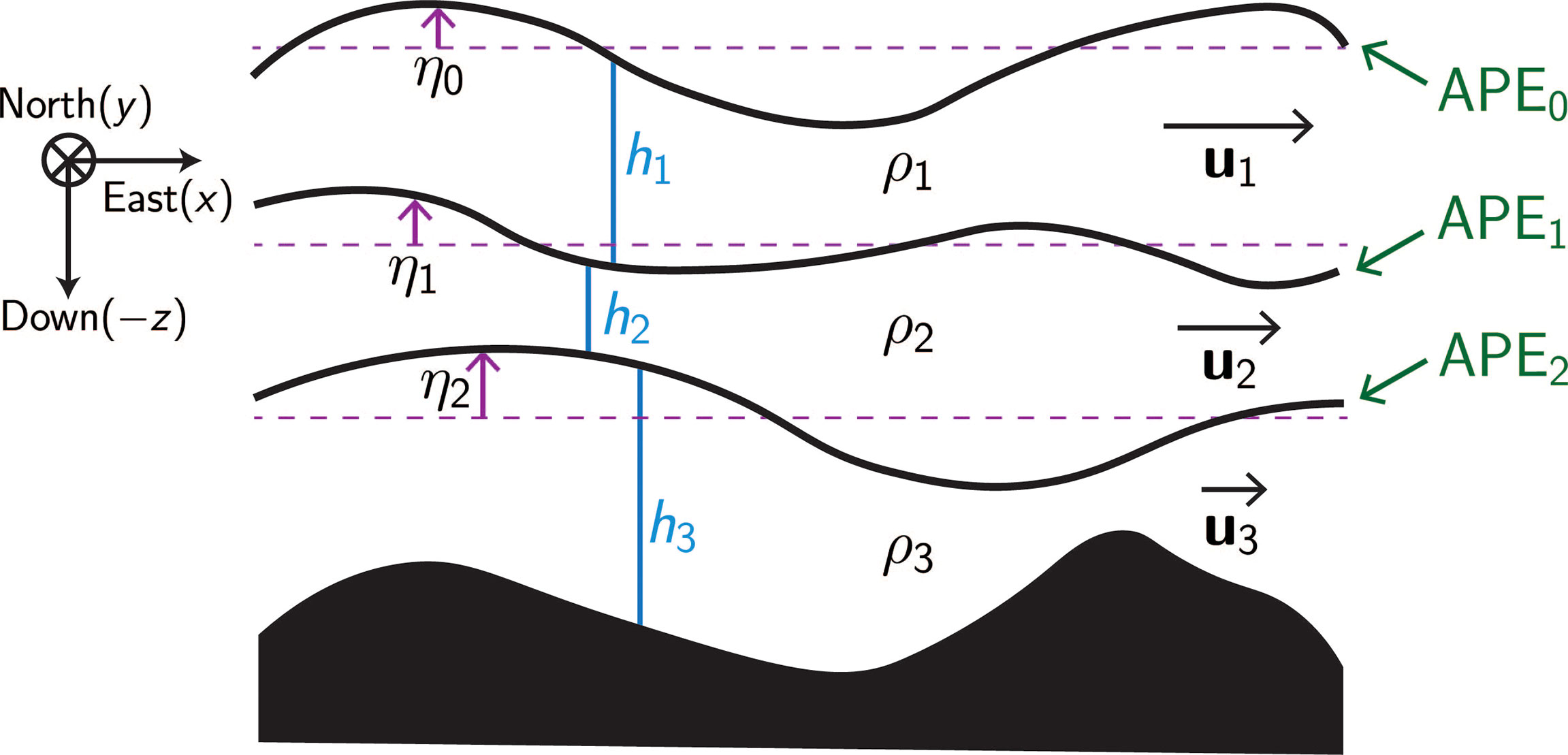
Figure 1 Schematic of three-layer diagram set-up configuration used in the energy conversion framework described in energy conversion framework. Layer i = 1 is at the top and layer i = 3 is at the bottom, so that ρ₁ < ρ₂ < ρ₃. Layer thicknesses h_i, horizontal velocities u_i, interface deviations n_j and corresponding available potential energy APE _j for each interface are labelled.

Here, the APE₀ is the available potential energy of the ocean’s free surface, defined by deviation η₀, and APE_j (j = 1, 2) is the available potential energy associated with each of the two internal interfaces between density layers of the ocean, with interface deviation η_j (Figure 1). The densities of the three layers are used to define reduced gravities g′₁= (ρ₂ – ρ₁)g/ρ₀ and g′₂ = (ρ₃ – ρ₂) g/ρ₀.

Following Aiki et al. (2016) and Barthel et al. (2017), the Navier Stokes equation for a rotating, Boussinesq fluid is used to describe the time dependence of the kinetic energy reservoirs, and is simplified by the layer-thickness continuity equation, under the assumption that the fluid is adiabatic. Time dependence of the APE reservoirs can also be calculated by differentiating η_j with respect to time, and simplifying with the Montgomery potential anomaly Φ_i (Cushman-Roisin and Beckers, 2011),

An equation for the advection of the Montgomery potential flux is also formulated (see Aiki et al. (2016) for details).

Having defined energy reservoirs and their time-dependence, Reynolds averaging is introduced to decompose quantities into mean and eddy quantities. The layer thicknesses and interface heights are decomposed as $h_{\text{i}}(x,t)=\overline{h_{\text{i}}}(x)+h_i^{\prime }(x,t)$, with overlined quantities the time-mean and primed quantities the deviation such that $\overline{h_i^{\prime }}=0$.

The time-mean available potential energy reservoirs are thus split into mean (MAPE) and eddy (EAPE) components:

For the horizontal velocities, we could use the same (Ᾱ, A′) Reynolds decomposition. However, following Bleck (1985), we instead choose to decompose the layer horizontal velocities into a thickness weighted mean velocity and deviation (Â, A"), defined as u_i = û_i + u_i", where the thickness weighted mean is expressed as

The use of this thickness-weighted mean is a key difference between the thickness-weighted energetics framework and that of Lorenz (1955). The kinetic energy is thus decomposed into mean (MKE) and eddy (EKE) components:

As in Aiki et al. (2016), the equations describing the time-dependence of these reservoirs are low-pass filtered in time, yielding equations describing the conversions into and out of the mean energy reservoirs. These mean equations are subtracted from the time-average of the original time-dependent equations, yielding equations describing conversions from the eddy energy reservoirs. The equation for the eddy kinetic energy in each layer is

Here, F_τ,i parameterises frictional forces (both interior viscosity and bottom drag) in each layer. The three-layer eddy kinetic energy budget, Eqn. (6), is identical to the two-layer framework of Barthel et al. (2017), but there are minor changes in the APE equations due to the addition of a third APE reservoir. Some terms appear in the equations for multiple energy reservoirs with opposite sign, indicating a transfer of energy between those reservoirs. An energy diagram can thus be constructed, in which conversions of energy act to link reservoirs (Figure 2). The mean and eddy Montgomery potential flux equations are also used to link reservoirs, where terms are not directly found in the equations for two different reservoirs. Two conversions linking mean and eddy reservoirs are identified:

● an energy conversion ${\hat{\mathit{u}}}_{\mathit{i}}·\overline{h_i^{\prime }\nabla {\varphi }_i^{\prime }}$ (blue arrows in Figure 2), related to the interfacial form stress, which plays a role in the momentum balance in the interior of the ocean (Ward and Hogg, 2011) by transferring momentum between density layers. This process is related to baroclinic instability (Aiki et al., 2016). This term is distinct from the baroclinic eddy kinetic energy generation term in Eqn. (6), $\overline{{\mathit{u}}_i^{″}·h_i\nabla {\varphi }_i^{″}}$ , which links the interfacial form stress conversion term to the eddy kinetic energy reservoir and thus represents generation of eddy kinetic energy via the baroclinic instability pathway.

● and an energy conversion related to the Reynolds stress ρ₀ (û_i ·∇)·($\overline{h_i{\mathbf{u}}_i^{″}\otimes {\mathbf{u}}_i^{″}}$) (orange arrows in Figure 2), which contains the Reynolds stress tensor. This conversion is related to horizontal velocity shear and thus barotropic instability (Barthel et al., 2017).

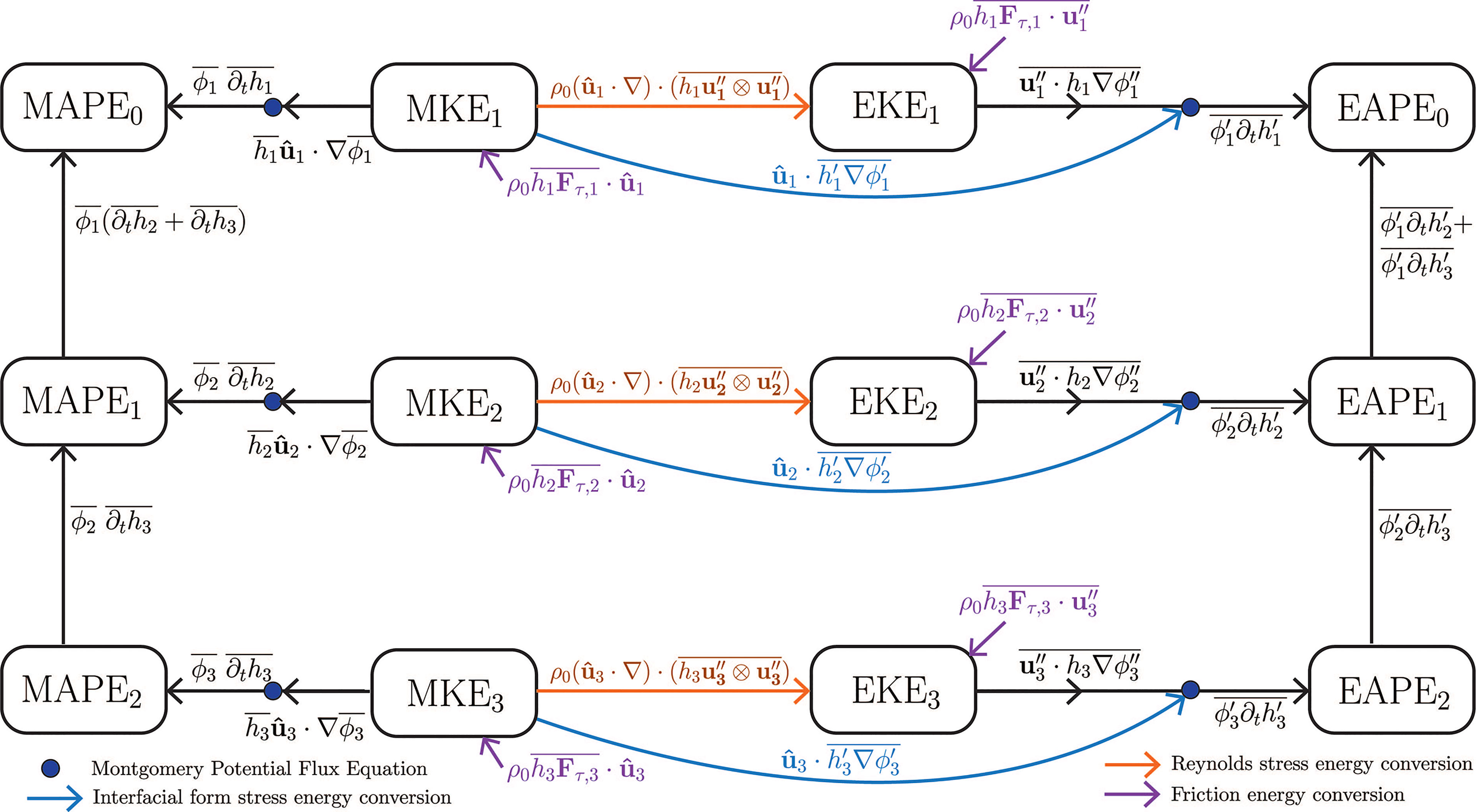
Figure 2 Energy conversions in a three-layer model. Arrows are drawn between energy reservoirs according to the thickness-weighted energy cycle equations, with the direction according to the sign in the equation (noting energy transfers can occur both ways). The blue and orange arrows show the conversions associated with interfacial form stress and Reynolds stress, corresponding to baroclinic and barotropic instabilities respectively. The navy dots indicate where Montgomery potential flux equations were used, to link the energy conversion terms surrounding the dots. The purple arrows indicate the terms related to friction. Advective terms are not shown.

These two conversion terms, the interfacial form stress conversion and Reynolds stress conversion, can be taken as indicators of the action of baroclinic and barotopic instabilities respectively. We calculate these terms, as well as the eddy kinetic energy generation terms in Eqn. (6), using output from a high-resolution ocean model to investigate the spatial distributions of instability processes involved in Southern Ocean upwelling.

Model Description

The model used in this study is a high-resolution global ocean and sea-ice model, ACCESS-OM2-01 (Kiss et al., 2020), which has 75 vertical levels and 0.1° spatial resolution. The model is hence eddy-resolving at Southern Ocean latitudes (Hallberg, 2013). ACCESS-OM2-01 uses ocean numerics and configurations based on the Modular Ocean Model version 5 (MOM5) (Griffies, 2012). The model is forced at the ocean surface by a repeat year forcing (May 1990-April 1991, a neutral year with regard to interannual climate modes (Stewart et al., 2020) of the JRA55-do atmospheric reanalysis (Tsujino et al., 2018). Using a repeat year forcing ensures the mean state of the ocean is relatively constant, for ease of calculating eddy-related quantities, and to ensure that interannual variability is due to oceanic processes. The model has been spun up for 270 years to decrease initial model drift, and the following 10 years of model output are analysed.

ACCESS-OM2-01 has an overturning circulation within the range of observation-derived estimates (Figure 3). The circulation can be analysed using the meridional overturning streamfunction, defined in density-latitude coordinates as

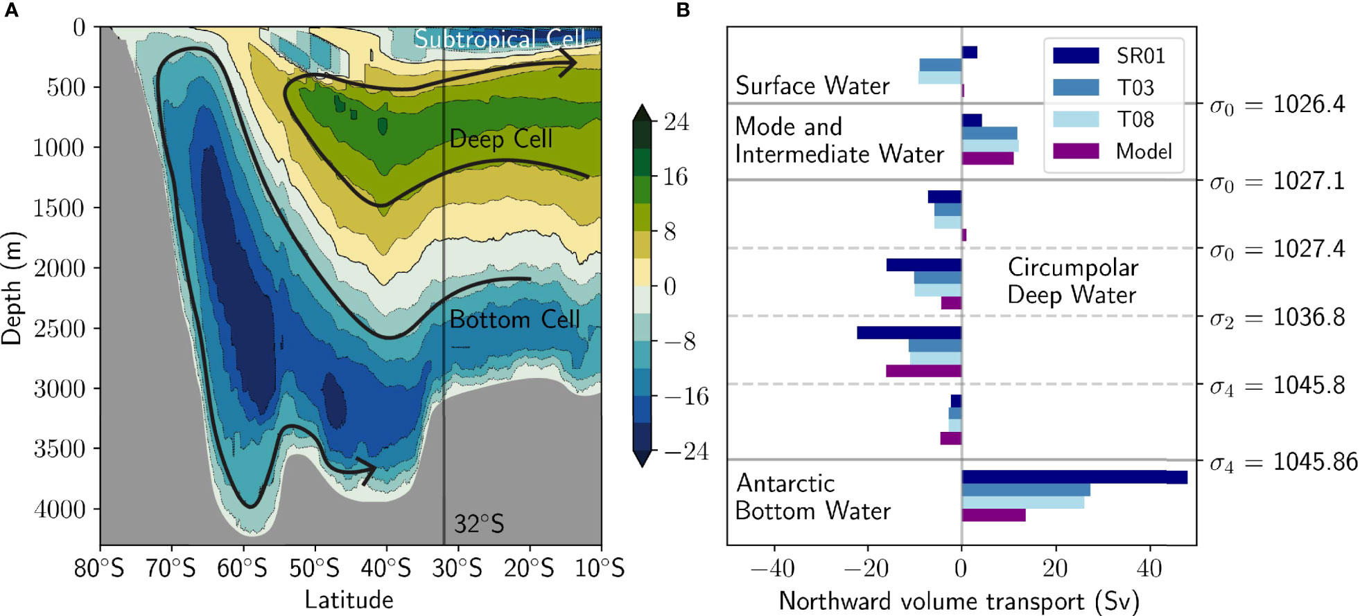
Figure 3 (A) Meridional residual overturning circulation streamfunction in depth coordinates, indicating the flow of water along contours. Flow can be interpreted to flow clockwise in green regions, and anticlockwise in blue regions along contours, as indicated conceptually by the black arrows. Topography is in grey. (B) Observation-derived estimates of transports at 30-40 °S reported in Sloyan and Rintoul (2001) (SR01), Talley et al. (2003) (T03), and Talley (2008) (T08) are compared to model transports at 32 °S. These transports are calculated for density classes defined by Talley et al. (2003). Additional resolution in density classes is provided for Circumpolar Deep Water compared with the other water mass classes.

where the ≡ symbol describes the equivalence of the depth coordinate (left) and density coordinate (right) calculations. This expression is the cumulative integral from the bottom of the ocean (σ_B) of the total northward transport in density layers $\overline{vh}(x,y,\sigma )$, integrated over all longitudes and time-averaged. Figure 3A shows the meridional overturning streamfunction calculated in σ₁ (potential density referenced to 1000 dbar) coordinates, mapped to the zonal-mean isopycnal depths. Flows can be interpreted to follow streamfunction contours (arrows). Note that this mapping is imperfect, because isopycnal depths vary with longitude so water exists at depths greater than the zonal mean, and is only provided for visualisation purposes.

Figure 3B shows the modelled volume transport at 32 °S in density classes defined by Talley et al. (2003), compared with three observation-derived inverse model estimates (Sloyan and Rintoul, 2001; Talley et al., 2003; Talley, 2008) between 30-40 °S. Additional resolution is provided for the Circumpolar Deep Water (southward moving, upwelling water). The modelled overturning circulation generally lies within the range of these sparse observational studies, but the model has too little Antarctic Bottom Water transport at 32°S compared with observations. Actual production of bottom water near Antarctica in ACCESS-OM2-01 compares well with observations (Moorman et al., 2020), an uncommon feat for ocean models, which often do not represent the process of bottom water formation near Antarctica accurately (Heuzé, 2021). The low bottom water transport at 32 °S is hence likely to be due to enhanced mixing in the model, owing to poor resolution of downslope flows and spurious numerical mixing. The modelled bottom water is thus over-mixed with lighter densities as it travels northwards, decreasing transport in the densest class.

We have only compared the model to observations at 32°S, where there is a range of observational studies, hence we cannot comment on the accuracy of the modelled overturning at the more southern Antarctic Circumpolar Current latitudes. However, since the modelled upwelling lies within the large range of observational estimates of the overturning circulation at 32°S, the modelled overturning circulation is likely to be sufficiently realistic for the purpose of understanding the physics involved in its upwelling arm. Additionally, Kiss et al. (2020) show good agreement of other diagnostics of ACCESS-OM2-01, such as temperature and salinity transects, Antarctic Circumpolar Current transport and sea-ice coverage, with observational datasets. Solodoch et al. (2022) provide further validation of the model in the Southern Ocean. The eddy kinetic energy distribution of ACCESS-OM2-01 is also similar in magnitude and spatial distribution to satellite observations (see Supplementary Figure S1).

Density Coordinate Transformation

The thickness-weighted energetics framework requires calculations in density coordinates, but ACCESS-OM2-01 output uses depth coordinates, and thus requires a vertical coordinate transformation. We choose 31 σ₁ density levels so that layers are 100-200 m thick (Figure 4A). We choose 1000 dbar (~1000 m) as the reference pressure for potential density, because the upwelling density range is approximately centred around 1000 m (Figure 3A). We recognise that neutral surfaces would be more accurate than potential density (McDougall, 1987; Jackett and McDougall, 1997), but they are computationally expensive.

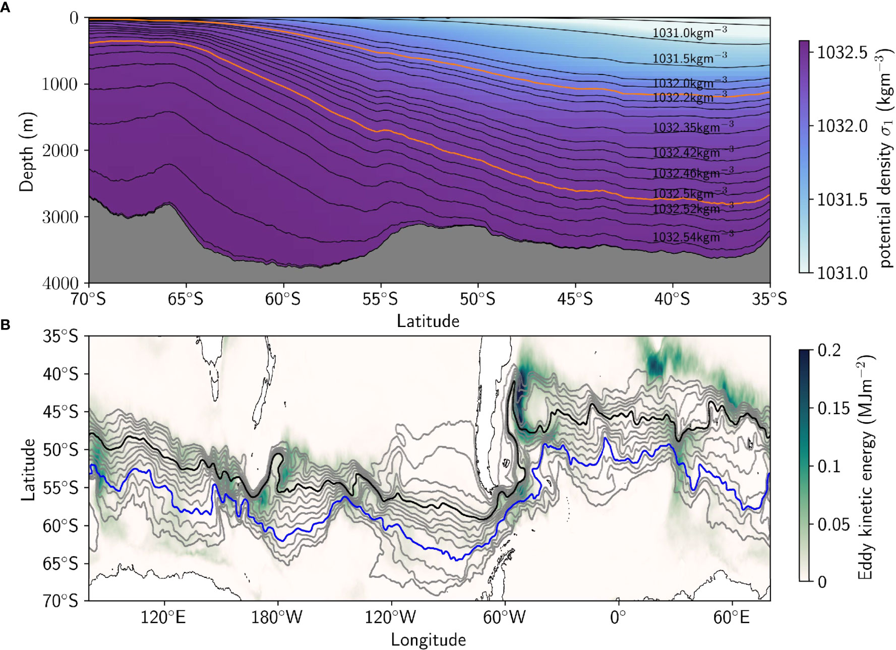
Figure 4 (A) Zonal mean isopycnal depths demonstrating the spacing of chosen σ₁ density bins (central value stated), which divide the ocean into 100-200m thick layers. Black lines indicate interfaces between the isopycnal layers. A subset of isopycnal layers are labelled with their density. The upwelling density range 1032.2 < σ₁ < 1032.5 kg m^-3 is highlighted in orange. (B) Selected circumpolar SSH contours (grey) with depth integrated eddy kinetic energy (green background). Every second SSH contour is shown, here spaced 0.1 m apart, with the -1.2 m SSH contour highlighted in blue and the -0.6 m SSH contour in black.

The ACCESS-OM2-01 model output is transformed into the 31 density levels following the binning method of Lee et al. (2007). The binning process is performed using daily averaged output. The high temporal resolution is important because correlations in fluctuations in layer thickness and velocity are used in energy and transport calculations. Sub-daily timescales are unlikely to be relevant for mesoscale dynamics in the Southern Ocean.

Reynolds Decomposition

The thickness-weighted energy conversion framework requires a Reynolds decomposition into time-mean and eddy quantities, as does the calculation of eddy transport as does the calculation of eddy transport. Eddy quantities are calculated as the deviations from a 10 year time-mean. Aiki and Richards (2008) find calculations of energy conversions to be robust to the choice of time-averaging. Seasonal variability in eddy kinetic energy is predominantly in the upper 100 m of the ocean (Rieck et al., 2015), far above upwelling processes, so we do not account for seasonality in the time-mean. Eddies in the Southern Ocean have lifetimes of around 6 months (Chelton et al., 2011), suggesting a 10 year time period would be sufficient to calculate accurate time-means that are not biased by a single eddy. This definition means the fluctuation term includes all variations, including seasonality, interannual variability and waves as well as turbulence.

Quantifying Upwelling

We define upwelling to be the eddy component of the volume transport across time-mean sea surface height (SSH) contours, which are indicative of Antarctic Circumpolar Current streamlines. The mean component of the volume transport in the interior density layers does not contribute to the net southward flow (shown later in the Results section), and therefore is not included in the analysis. Computing the eddy transport across SSH contours, rather than across lines of constant latitude, removes the majority of the ACC flow from the calculated upwelling transport. Removing the mean transport also minimises the contribution of ACC standing meanders to the upwelling transport across SSH contours. The mean ACC flow at depth does not exactly follow SSH contours,but we find that other choices of contours, such as Montgomery potential or isopycnal depth contours, yield similar results (not shown). The cross-contour volume transport across a contour $\mathcal{C}$ of scalar field $\mathcal{S}$ through an area dA tangent to the contour is

For a density layer in the ocean with layer thickness h, and nearly horizontal flows, this reduces to

where we have taken dA to extend throughout the layer, and the vector ${\mathbf{n}}_{\mathbf{s}}=\nabla S/\left|\nabla S\right|$.

The quantity t(ρ,x,$\mathcal{C}$) has units of area per unit time, and is properly a linear density of volume transport, but for simplicity we refer to it also as the cross-contour volume transport. When integrated over all points along a contour $\mathcal{C}$, we obtain the circumpolar transport T(ρ,$\mathcal{C}$). The three-dimensional cross-contour volume transport t can be decomposed via a Reynolds decomposition into mean and eddy components, of which the eddy component, t_eddy, is our measure of upwelling

The eddy cross-contour volume transport is calculated for 29 evenly spaced SSH contours between -0.1 and -1.5 m (Figure 4B), which cover the latitudinal extent of the Antarctic Circumpolar Current. The cross-contour transport is computed across the faces of the discrete model tracer grid cells to guarantee exact closed circumpolar contours. The eddy transport is smoothed with a 10 along-contour grid point running average to reduce noise (Figure 5A). This can be thought of as reducing the influence of the rotational component of eddy transport, which obscures the physically relevant divergent component (Lau and Wallace, 1979). The decomposition is imperfect (Griesel et al., 2009) as only a circumpolar average can truly remove all of the rotational eddy transport, and thus we do not claim to have exactly calculated the divergent eddy transport (note that no such divergent-rotational decomposition is perfect, as solutions are not unique in the presence of boundary conditions (Fox-Kemper et al., 2003). However, we expect that including part of the rotational eddy transport will only increase noise, and that hence the significance of any results would likely increase if the rotational component had been entirely removed. The choice of 10 grid cell smoothing is not unique and is chosen to be of a similar length scale to observed eddy sizes (Klocker and Abernathey, 2014), but our results are not sensitive to this choice.

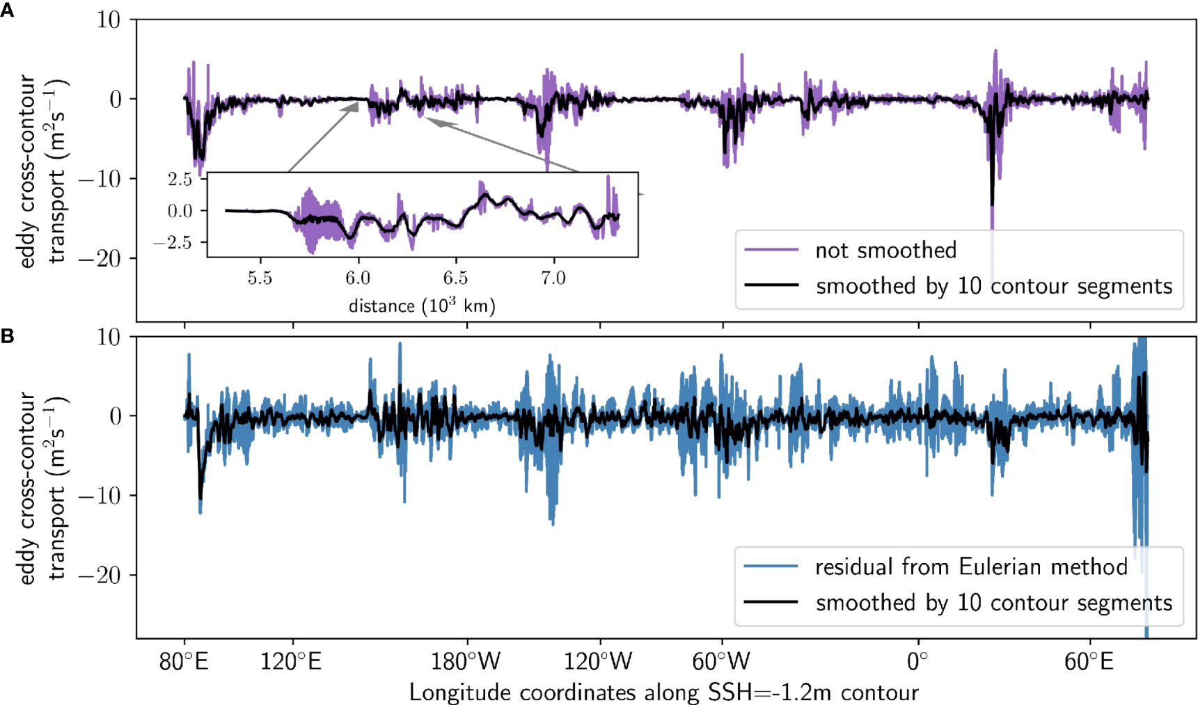
Figure 5 (A) Cross-contour eddy transport t_eddy, calculated according to Eqn. (10) across the -1.2m SSH contour summed over the density range 1032.2 < σ₁ < 1032.5 kg m^-3, for unsmoothed (colours) and smoothed (black, running average over 10 contour segments) cases. (B) as for panel A, but with the eddy transport calculated using the traditional method as the difference between the residual overturning in σ₁ coordinates, and the Eulerian mean (i.e. depth space) overturning mapped to σ₁ coordinates.

Note that our definition of eddy transport (Eqn. 10) differs from the more traditional definitions of overturning circulation eddy-mean decompositions (e.g. Wolfe and Cessi, 2009). In the traditional method, the eddy component is taken as the difference between the residual transport in density coordinates and the time-mean Eulerian transport in depth coordinates mapped to density coordinates. The time-mean Eulerian transport calculation therefore includes velocity contributions from layers outside the isopycnal of interest. In contrast, our isopycnal mean method uses the time mean velocity $\overline{\mathbf{u}}$ within a single density layer, with velocities averaged across a range of depths following vertical movement of the isopycnal. The streamfunction associated with mean transports calculated via the isopycnal mean method will not be closed due to temporal variation in the range of isopycnals present, and hence the isopycnal mean method is not ideal for streamfunction calculations, but we argue that this method is more physically justified for the purposes of analysing transport in the upwelling density range of the ocean. We present the isopycnal mean method in Figure 5A and the traditional method in Figure 5B, the latter of which contains more noise and less prominent upwelling hotspots, even after the same smoothing filter was applied. We thus use only density coordinates in all calculations.

We analyse upwelling dynamics over a density range that is representative of the zonally averaged upwelling (bounded by the orange contours in Figure 4A). We refer to this density range as the ‘upwelling arm’. The density range is chosen to select densities of water that, in the circumpolar average, have net eddy transport orientated southward and do not intersect the surface or ocean bottom during the 10 year simulation period. These criteria ensure that northward flowing bottom water and surface layer water are not included, as different dynamics are present in these boundary regions of the ocean. Specifically, flows are more likely to include diabatic components at boundaries, which contradicts the adiabatic assumption underpinning the thickness-weighted energetics framework. Outcropping density layers also need not be considered. Since isopycnals slope in the Southern Ocean, the density range satisfying these criteria varies with latitude and SSH contour. We thus choose a density range such that all contours with SSH less than or equal to -0.6 m satisfy the two criteria, resulting in the upwelling arm density range 1032.2 < σ₁ < 1032.5 kg m^-3.

Results

Importance of Topographic Hotspots of Upwelling

The meridional overturning streamfunction in σ₁-latitude coordinates is presented in Figure 6A. Streamfunction contours are approximately horizontal in density-latitude space except near the surface (lightest colours), indicating that flow occurs nearly a diabatically along isopycnals. Thus, assumptions that upwelling occurs along isopycnals are valid except near the surface. The decomposition of the residual overturning circulation into mean and eddy components is shown in Figures 6B, C respectively, using the same Reynolds decomposition as for eddy transport which computes the mean overturning from the mean velocity on isopycnals, rather than the usual depth-space Eulerian mean calculation (see Methods). Southward eddy transport (Figure 6C) is intensified in the upwelling arm (between the horizontal orange lines) and between 500-2000 m depth (dotted and dashed grey lines).

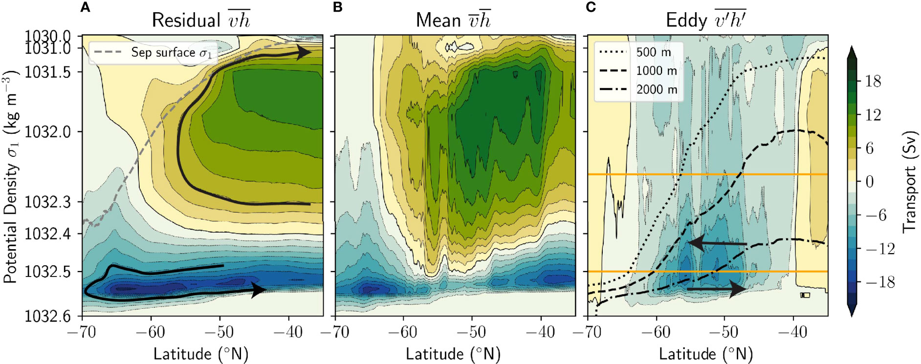
Figure 6 Zonally averaged residual overturning streamfunction (A), and its decomposition into mean (B) and eddy (C) terms, averaged over 10 years. Density (σ₁) coordinates are used – note the nonlinear vertical axis. Arrows indicate the direction of flows, which follow streamfunction contours. Positive streamfunction values indicate clockwise circulation. In panel A, the zonal and time averaged September surface density is shown to indicate the seasonally densest surface waters. In panel C, the orange lines indicate the upwelling arm density range, and the black lines the average densities at depths 500 m, 1000 m and 2000 m, as indicated in the legend.

The analysis of zonally integrated eddy transport is useful for quantifying the total upwelling. However, upwelling is known to vary with longitude (Tamsitt et al., 2017). We first consider the transport along a single contour – the -1.2 m SSH contour, highlighted in Figure 4B – to illustrate the spatial distributions of eddy and mean transport contributions. The horizontal spatial distribution of eddy upwelling across the -1.2 m SSH contour (Figure 7A) shows that southward eddy transport is non-uniform, and enhanced in regions that are colocated with or are downstream of topographic features. The along-contour cumulative integrals of eddy, mean and total transport across the -1.2 m SSH contour are shown in Figure 7B. There are five regions of high southward eddy transport (black) that occur near topography, defined by large changes in the cumulative integral. We refer to these regions as topographic hotspots of upwelling. The residual (blue) transport across the -1.2 m SSH contour is also southward, consistent with the zonally averaged the residual overturning streamfunction (Figure 6), whilst the mean (red) transport is noisy and small in the along-contour integral. The small-scale variation in mean and total transport, due to the mean Antarctic Circumpolar Current crossing the SSH contours, is not present in the eddy transport. The smooth eddy transport suggests that the Reynolds decomposition method isolates the eddy transport signal from the mean Antarctic Circumpolar Current, providing confidence that the cross-contour eddy transport method accurately estimates upwelling. There is a total of 19 Sv of southward eddy transport across the -1.2 m SSH contour, integrated vertically over the upwelling arm (Figure 7B). The eddy transport in the hotspot regions (grey bars) dominates the transport; the eddy transport in these regions contributes 76% to the total eddy transport, but occurs in only 28% of the circumpolar longitude range for this contour. A similar dominance of hotspot regions occurs across the majority of Southern Ocean SSH contours.

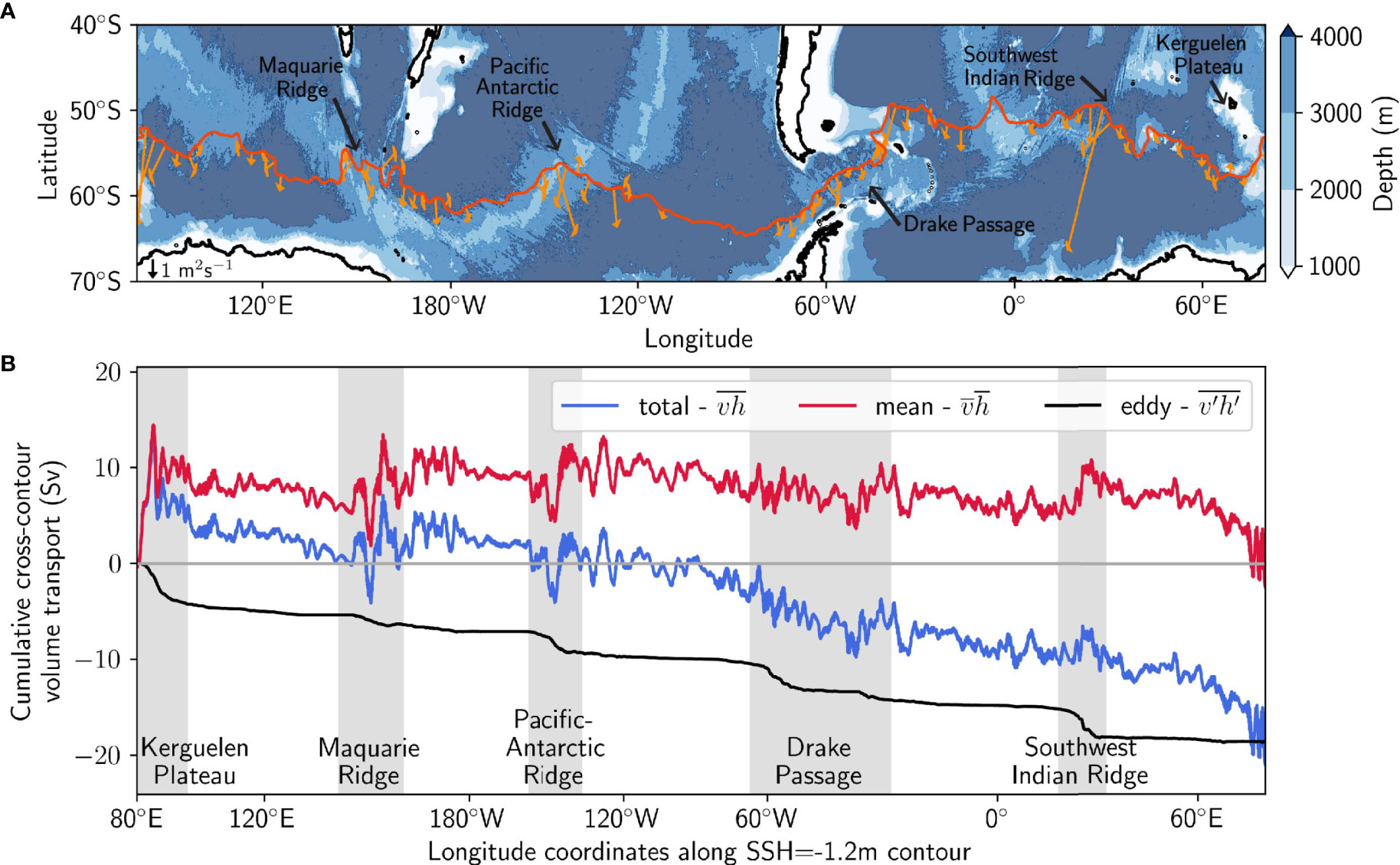
Figure 7 (A) Eddy transport t_eddy(ρ, x, C) integrated over the upwelling arm of the ocean, illustrated by arrows every 5° on the -1.2 m SSH contour, which show the direction and size of cross-contour eddy transport (an arrow is shown for scale in the bottom left corner). Transports with magnitude less than 0.2 m²s^-1 are not shown. Background shows bathymetry. (B) Cumulative integrals from west to east along the SSH contour of total, mean and eddy cross-contour volume transport, for the -1.2 m SSH contour. Transports are vertically integrated over the density range of the upwelling arm. Grey bars highlight the eddy upwelling hotspots.

Upwelling is spatially variable, so we analyse the spatial distribution of upwelling across SSH contours, densities and depths at each hotspot. Figure 8A shows the eddy transport integrated along circumpolar contours for each density bin, T_eddy(ρ, $\mathcal{C}$). The SSH axis ($\mathcal{C}$) is a proxy for latitude. The upper black line is the along-contour average surface density, and the lower line indicates where T_eddy > 0 (northward-flowing bottom water not associated with upwelling). Integrating between these black lines gives upwelling as a function of SSH contour, expressed as ∑ ρ_top<ρ<ρ_bottomT(ρ, $\mathcal{C}$_hotspot). Figure 8C shows this distribution of upwelling across SSH contours at each hotspot, $\mathcal{C}$_hotspot. Hotspots are defined by the following longitude ranges: Macquarie Ridge 130 °E-155 °W, Pacific-Antarctic Ridge 155 °W-100 °W, Drake Passage 80 °W-5 °E, Southwest Indian Ridge 5 °E-55 °E, and Kerguelen Plateau 55 °E-130 °E. Upwelling occurs over the whole range of sea surface contours, indicating upwelling occurs at all points across the Antarctic Circumpolar Current. However, the SSH contours where upwelling is maximised depend on the hotspot, with the Southwest Indian Ridge, Kerguelen Plateau and Pacific Antarctic Ridge having more upwelling over southern contours and Drake Passage and Macquarie Ridge in central contours. Furthermore, Drake Passage is the hotspot with the most upwelling transport (Figure 8C), which is attributed to its substantial topography and longitudinal extent (Figure 7A), while the other hotspots have similar contributions to the circumpolar upwelling transport.

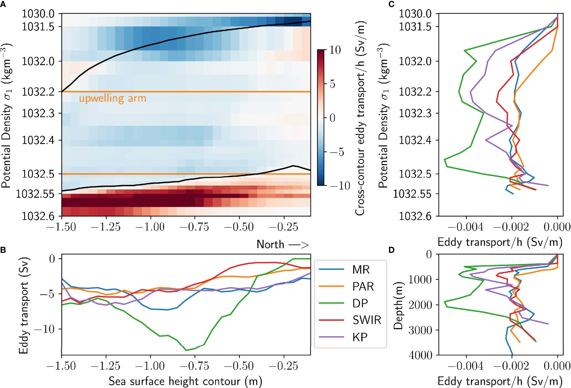
Figure 8 Cross-contour eddy transport in each isopycnal layer integrated along circumpolar SSH contours, T(ρ, C) (A). The upper black line is the average surface density of each SSH contour, and the lower black line is the density bounding southward eddy transport, averaged along circumpolar contours. For each hotspot, the transport between the (hotspot-equivalent) two black lines is averaged over all contours (B) and integrated over upwelling densities (C) giving eddy transport distributions in density and SSH contour space respectively. The density distribution from B is mapped into depth space in (D). The hotspots are Macquarie Ridge (MR), Pacific-Antarctic Ridge (PAR), Drake Passage (DP), Southwest Indian Ridge (SWIR), and Kerguelen Plateau (KP).

Figure 8B shows the eddy transport summed along contours at each hotspot T(ρ, $\mathcal{C}$_hotspot) between the black lines of Figure 8A, averaged over all the SSH contours $\mathcal{C}$_hotspot and normalised by the average layer thickness h, and hence shows upwelling in density space. The density axis of Figure 8B is then mapped back into depth space (Figure 8D). The density ranges of eddy upwelling hotspots (Figure 8B), are similar with small variations. Kerguelen Plateau in particular has its upwelling skewed to lighter densities and shallower depths (Figure 8D) than the other hotspots. The topography of Kerguelen Plateau is shallower than other hotspots, with large parts of the plateau shallower than 1000 m (Figure 7A). The interaction of the flow with topography at different depths is thus likely to be relevant to the density of upwelling water. Figure 8 shows that upwelling occurs at densities outside of the upwelling arm density range. However, the eddy transport in the upwelling arm density range accounts for ~75% of the total southward eddy transport, indicating the upwelling density arm is a sufficient representation of upwelling water.

Interfacial Form Stress Conversion and Upwelling

As motivated in the Energy Conversion Framework section, we use the interfacial form stress conversion calculated from a layer-thickness energetics framework to indicate the spatial distribution of baroclinic instability in the high-resolution model. The interfacial form stress conversion (blue arrows in Figure 2) was calculated in the 31 levels of the transformed ACCESS-OM2-01 model output. From 35-70°S, the interfacial form stress conversion results in 0.29 TW converted from mean to eddy energy, consistent with the action of baroclinic instability. The spatial distribution of eddy transport is compared with contours of the interfacial form stress conversion, for the five topographic hotspots of upwelling (Figure 9), and shows that the energy conversion is enhanced in the same locations as upwelling. Since eddy transport is calculated over SSH contours, the eddy transport distributions have been interpolated between SSH contours onto the model grid to better compare with the interfacial form stress conversion, which is computed in every horizontal grid cell. Grid cells lying between SSH contours are assigned a transport weighted by the distance between the two closest points on adjacent contours. The resultant spatial distribution of eddy transport is not uniquely defined at grid points between contours since other interpolation methods exist, but provides a visual guide. Southward eddy transport regions (blue shading) have a striking spatial correspondence with positive interfacial form stress conversion values (purple contours), and conversely northward eddy transport (red colours) tends to be located where the interfacial form stress conversion is negative (orange/yellow contours). The spatial correspondence is best highlighted at the Southwest Indian Ridge hotspot (Figure 9A). There are, however, regions where the correspondence is less strong (e.g. the north-western part of the Pacific-Antarctic Ridge, Figure 9D), which may be explained by shortcomings in the assumption of adiabatic and geostrophic mean flows (see Discussion).

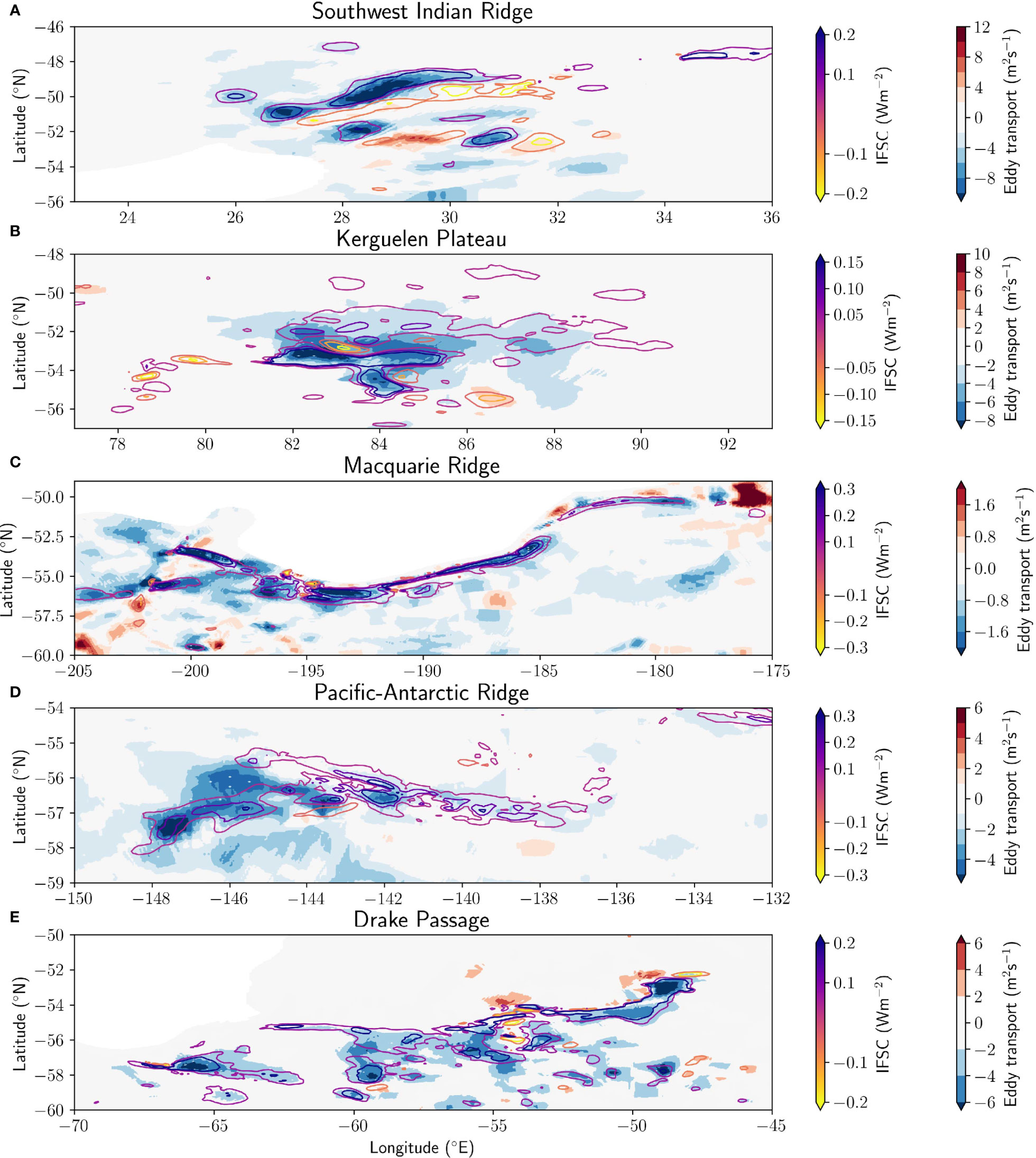
Figure 9 Cross-contour eddy transport (background map, blue is southward cross-contour transport) and interfacial form stress energy conversion (IFSC) (coloured contours), integrated over the upwelling arm density range for each of the five hotspots: (A) Macquarie Ridge, (B) Pacific-Antarctic Ridge, (C) Drake Passage, (D) Southwest Indian Ridge, and (E) Kerguelen Plateau.

To better quantify the visible spatial correspondence between eddy transport and the interfacial form stress conversion, we compare the distributions of southward eddy transport and the interfacial form stress conversion along the -1.2 m SSH contour (Figure 10A). A lag-correlation analysis (Figure 10B) shows the Pearson regression correlation coefficient for each spatial lag between the two fields, where a positive lag distance indicates that the transport is upstream of the energy term. Regions of significance greater than 95% confidence are highlighted, taking into account internal correlations in the spatial distributions (Santer et al., 2000). There is a significant correlation (Pearson regresssion correlation coefficient r = 0.80) between the interfacial form stress conversion and eddy transport with zero lag (Figure 10B) for the -1.2 m SSH contour. Similar results (0.63 ≤ r ≤ 0.80) hold for all other contours with SSH less than -0.6 m. In comparison, the Reynolds stress conversion associated with barotropic instability (orange arrows in energy budget, Figure 2) is enhanced in the same regions as eddy transport, but is not correlated (Figure 10C), with maximum correlation r = 0.26 for the -1.2 m SSH contour (Figure 10D) and r ≤ 0.53 for other contours. The high spatial correspondence between the interfacial form stress conversion and eddy transport indicates that the two fields are dynamically linked, and thus that upwelling is driven by baroclinic instability. This result is consistent with the idealised study of Barthel et al. (2022). Quantifying this baroclinic conversion could thus be an avenue for improving parameterisations of eddy transport in coarse resolution models.

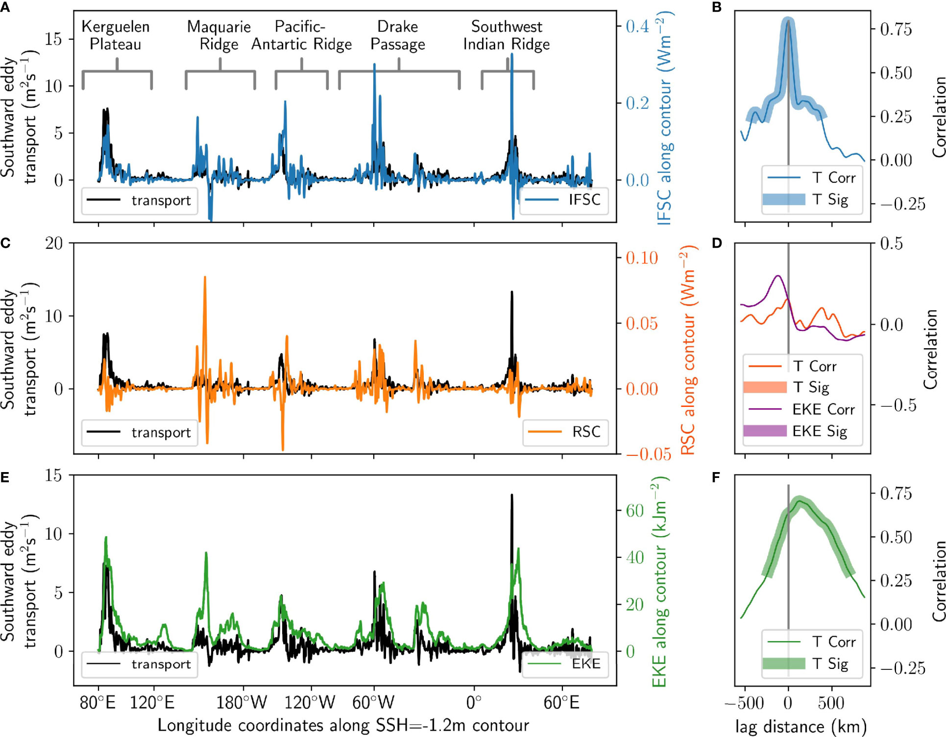
Figure 10 Southward eddy transport vertically integrated over the upwelling arm (black, T) compared with (A) the interfacial form stress energy conversion (IFSC), (C) eddy kinetic energy and (E) Reynolds stress energy conversion (RSC) along the -1.2 m SSH contour. The spatial lag correlations are shown in the right panels (B, D, F), with highlighting indicating significant correlations with 95% confidence. A correlation peaking at a positive lag distance means the eddy transport (indicated by T, or in the case of the purple line, eddy kinetic energy indicated by EKE) is upstream of the energy term. The additional purple line in panel (D), the eddy kinetic energy lag distance, compares the eddy kinetic energy and Reynolds stress conversion, where a positive lag indicates the eddy kinetic energy leads the Reynolds stress conversion. Note the change in sign of the eddy transport axes compared to previous analyses, for improved visualisation of the correlations.

Eddy Kinetic Energy Downstream of Upwelling

Past idealised and observational studies have suggested that, like upwelling, eddy kinetic energy is enhanced downstream of topography (Chelton et al., 1990), but that there is a spatial offset between eddy kinetic energy and upwelling (Barthel et al., 2022), eddy heat fluxes (Abernathey and Cessi, 2014; Foppert et al., 2017), and baroclinic activity (Bischoff and Thompson, 2014; Chapman et al., 2015). We investigate this phenomenon using ACCESS-OM2-01. The modelled eddy kinetic energy distribution (Figure 4B) is spatially variable, and enhanced in similar regions to the upwelling. Figure 10E compares the along-contour distribution of eddy transport and eddy kinetic energy for the -1.2 m SSH contour. There is a significant correlation (r = 0.71; Figure 10F), maximised at a lag distance of 126 km. When this peak distance is averaged over all contours with sea surface heights less than -0.6 m, the eddy kinetic energy is found to lag the eddy transport by 110 ± 20 km (where the uncertainty is the standard error in the mean), and has maximum lag correlations of 0.50 ≤ r ≤ 0.71. This distance is in accordance with an observational study of eddy heat fluxes (Foppert et al., 2017). For parameterisations of eddies that use eddy kinetic energy, this is an important result, as the downstream distance only covers two grid cells in a coarse 1° model, and is thus unlikely to negatively affect the accuracy of parameterised eddy transport. For eddy parameterisations used in models with a resolution finer than 1°, the spatial offset between EKE and eddy transport may need to be considered.

The same analysis can be performed at each hotspot for contours where there is a significant correlation between eddy kinetic energy and upwelling, yielding downstream distances of 50 ± 40 km at Macquarie Ridge, 70 ± 10 km at the Pacific-Antarctic Ridge, 100 ± 20 km at Drake Passage, 230 ± 60 km at the Southwest Indian Ridge and 80 ± 20 km at Kerguelen Plateau. Individual contours at each hotspot deviate from these mean distances, but eddy kinetic energy is persistently downstream of eddy transport.

Mechanisms for Downstream Eddy Kinetic Energy

We have shown that in ACCESS-OM2-01, eddy kinetic energy maxima are found downstream of upwelling hotspots. Since upwelling and the interfacial form stress conversion are highly correlated, the eddy kinetic energy is also found downstream of the baroclinic energy conversion process. There are several candidate mechanisms for this downstream offset that have been suggested in the literature, including the advection of eddies (and therefore eddy kinetic energy) (Thompson and Naveira Garabato, 2014), the advection of pressure perturbations (Montgomery potential flux in a layered framework) (Chang and Orlanski, 1993; Abernathey and Cessi, 2014; Chapman et al., 2015), the barotropic generation acting downstream of the baroclinic generation (Barthel et al., 2022), a time-delay between the instability process and eddy kinetic energy generation (Chen et al., 2016) (which via advection of eddy potential energy due to barotropic eddies results in a spatial offset), and bathymetric configuration and eddy-mean flow interactions (Foppert et al., 2017). Using the thickness-weighted energetics framework, the plausibility of two mechanisms, relating to the advection of eddy kinetic energy and the action of barotropic instability, can be investigated.

Eddy kinetic energy advection terms and the Reynolds stress conversion associated with barotropic instability can be identified in the eddy kinetic energy evolution equation (6). When integrated over the full depth of the ocean and between sea surface heights -0.6 m and -1.5 m, the advective terms contribute 0.51 GW to energy conversions, and the Reynolds stress conversion 2.8 GW. These conversions are small compared with the baroclinic eddy kinetic energy generation term, $\overline{{\mathbf{u}}_{\mathbf{i}}^{″}·h_i\nabla {\varphi }_i^{″}}$, which when integrated over the same region is three orders of magnitude larger at 1.3 TW. The small magnitudes of the advective and Reynolds stress conversion terms in this region are only partly due to cancellation of local positive and negative conversions – the local absolute value of the energy conversions integrated over the same SSH range is 0.18 TW for the advective terms, 0.17 TW for the Reynolds stress conversion and much larger at 10 TW for the baroclinic eddy kinetic energy generation term. Furthermore, there is no significant (to 95% confidence) correlation between the eddy kinetic energy and Reynolds stress conversion along SSH contours (Figure 10D). Correlation analyses hence do not support a mechanism whereby the barotropic instability facilitated eddy kinetic energy generation downstream of eddy transport. Our analysis thus suggests that neither the downstream advection of eddy kinetic energy, nor the downstream action of barotropic instability from baroclinic instability, are likely to be primary mechanisms for creating the spatial offset between upwelling and eddy kinetic energy. Our findings show a reduced magnitude and thus importance of the barotropic energy conversion compared to the idealised two-layer model analysis of Barthel et al. (2022) – the authors acknowledge their simplified set-up may overstimulate barotropic instability (Youngs et al., 2017; Barthel et al., 2017; Barthel et al., 2022). This difference suggests that the many-layered, global ocean model employed here experiences different dynamics to the idealised model, and thus that it is important to verify the findings of idealised models in more realistic global models.

We have not verified other proposed mechanisms for downstream eddy kinetic energy, but suggest that future work could use a high-resolution global ocean model to investigate the downstream advection of pressure perturbations using wave activity flux theory (Takaya and Nakamura, 2001; Chapman et al., 2015). The wave activity flux framework includes an ageostrophic Montgomery potential flux term that has been suggested in idealised studies (Chang and Orlanski, 1993; Chapman et al., 2015) and observations (Foppert, 2019) to dominate horizontal wave activity transport. Via this mechanism, pressure perturbations are quickly swept downstream where they convert eddy potential energy into eddy kinetic energy (Abernathey and Cessi, 2014). Our time-mean energy conversion analysis is also unsuitable for examining timescales between baroclinic instability and eddy kinetic energy generation, along the lines of Chen et al. (2016), and is a subject for future work.

Discussion

This study uses output from a high-resolution global ocean model to show that five topographic hotspots dominate the upwelling in the Southern Ocean. These hotspots are controlled by baroclinic instability, since eddy transport is highly correlated with the interfacial form stress energy conversion. Regions of the ocean where baroclinic instability acts to convert mean energy reservoirs into eddy energy are thus the same locations where enhanced upwelling occurs. Eddy kinetic energy is also enhanced downstream of topography, but maximised on average 110 km downstream of upwelling. These key findings are summarised in a schematic in Figure 11.

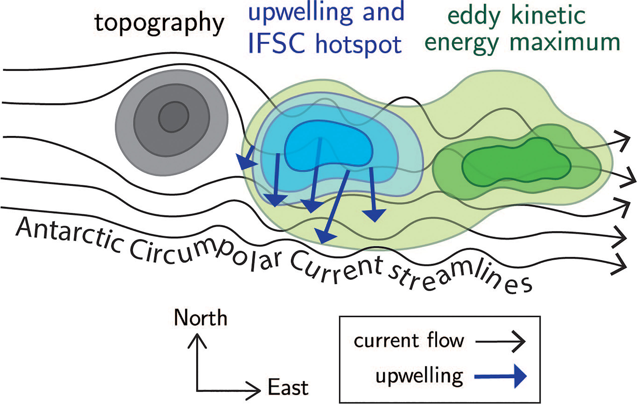
Figure 11 Schematic of upwelling hotspot dynamics, from a bird’s eye view perspective. The Antarctic Circumpolar Current (black arrows) becomes unstable downstream of topographic obstacles (grey contours), resulting in an upwelling and baroclinic conversion (IFSC) hotspot (blue arrows and contours). The eddy kinetic energy (green contours) is also enhanced downstream of topography but is maximised further downstream.

The mechanisms that create eddy kinetic energy downstream of upwelling, and thus why the downstream distance differs with each hotspot, remain unclear, but our energetics analysis suggests that neither the advection of eddy kinetic energy nor the barotropic instability conversion acting downstream of upwelling are likely to be the main cause. We find that the baroclinic conversion is at least an order of magnitude larger than the barotropic conversion, in contrast to idealised studies. The main implication of our work in relation to eddy parameterisation is that a metric or budget that describes the baroclinic conversion could be a useful avenue for improving eddy transport parameterisations. Eddy kinetic energy, whilst found downstream of upwelling hotspots, is also highly correlated with upwelling and thus appears to be an appropriate alternative eddy parameterisation (e.g. Jansen et al., 2015).

The methods of this study yield robust results, but contain caveats worth mentioning. Assumptions made in the formulation of the layer-thickness energy conversions assume that flows are adiabatic, and the quantification of upwelling assume that the mean flow is geostrophic, and thus follows SSH contours. Neither of these assumptions are strictly true – diapycnal mixing, whilst weak, exists in the Southern Ocean (Ledwell et al., 2011), and is enhanced above rough topography where internal waves are radiated upwards and break (Nikurashin and Ferrari, 2010; Naveira Garabato et al., 2016). The mean flow meanders across SSH contours at depth (red line, Figure 7B). These factors are likely responsible for regional anomalies where a significant correlation between upwelling and the baroclinic conversion did not hold (e.g. the north-western part of the Pacific Antarctic Ridge, Figure 9D). Improvements to the method could use a more precise density coordinate method, such as neutral density (Jackett and McDougall, 1997). The eddy fluxes could also be computed using other methods, such as down-gradient eddy fluxes (Marshall and Shutts, 1981), though as with our method, these calculations are complicated by the imperfect divergent-rotational Helmholtz decomposition in a finite domain (Fox-Kemper et al., 2003).

This study has demonstrated the utility of a high-resolution global ocean model in examining the dynamics of topographic hotspots of upwelling. Further work could investigate the time-variability of these processes under realistic atmospheric forcings, and the response between wind forcing, the interfacial form stress conversion, upwelling and eddy kinetic energy generation. Understanding the timescales on which upwelling processes act and are modified by climate and intrinsic forcing in realistic, high-resolution global ocean models will help to improve future predictions of the meridional exchange of heat and carbon transport in the Southern Ocean and their implications on global climate.

Data Availability Statement

The datasets generated and analysed in this study can be found in the Zenodo repository https://doi.org/10.5281/zenodo.5847602. Notebooks used to process, analyse and present data are available at https://github.com/claireyung/Topographic_Hotspots_Upwelling-Paper_Code.

Author Contributions

CY performed the analysis and wrote the manuscript. AM conceived the study and contributed to the analysis. All authors contributed to the study design and interpretation of results, as well as editing and revising the manuscript. All authors contributed to the article and approved the submitted version.

Funding

AM was supported by the Australian Research Council (ARC) DECRA Fellowship DE170100184. CY was supported by the Australian National University National University Scholarship, and the ARC Centre of Excellence for Climate Extremes Honours Scholarship.

Conflict of Interest

The authors declare that the research was conducted in the absence of any commercial or financial relationships that could be construed as a potential conflict of interest.

Publisher’s Note

All claims expressed in this article are solely those of the authors and do not necessarily represent those of their affiliated organizations, or those of the publisher, the editors and the reviewers. Any product that may be evaluated in this article, or claim that may be made by its manufacturer, is not guaranteed or endorsed by the publisher.

Acknowledgments

This research was undertaken on the National Computational Infrastructure (NCI) in Canberra, Australia, which is supported by the Australian Government. The authors thank the Consortium for Ocean-Sea Ice Modelling in Australia (COSIMA; http://www.cosima.org.au) for making the ACCESS-OM2 suite of models available at https://github.com/COSIMA/access-om2. We acknowledge Josué Martínez-Moreno for providing processed satellite observations of eddy kinetic energy.

Supplementary Material

The Supplementary Material for this article can be found online at: https://www.frontiersin.org/articles/10.3389/fmars.2022.855785/full#supplementary-material

References

Abernathey R., Cessi P. (2014). Topographic Enhancement of Eddy Efficiency in Baroclinic Equilibration. J. Phys. Oceanogr. 44, 2107–2126. doi: 10.1175/JPO-D-14-0014.1
Aiki H., Richards K. J. (2008). Energetics of the Global Ocean: The Role of Layer-Thickness Form Drag. J. Phys. Oceanogr. 38, 1845–1869. doi: 10.1175/2008JPO3820.1
Aiki H., Zhai X., Greatbatch R. J. (2016). Energetics of the Global Ocean : The Role of Mesoscale Eddies. Indo-Pacific Climate Variability and Predictability 7, 109–134. doi: 10.1142/9789814696623_0004
Armour K. C., Marshall J., Scott J. R., Donohoe A., Newsom E. R. (2016). Southern Ocean Warming Delayed by Circumpolar Upwelling and Equatorward Transport. Nat. Geosci. 9, 549–554. doi: 10.1038/ngeo2731
Barthel A., Hogg A. M., Waterman S., Keating S. R. (2017). Jet-Topography Interactions Affect Energy Pathways to the Deep Southern Ocean. J. Phys. Oceanogr. 47, 1799–1816. doi: 10.1175/JPO-D-16-0220.1
Barthel A., Hogg A. M., Waterman S., Keating S. R. (2022). Baroclinic Control of Southern Ocean Eddy Upwelling Near Topography. Geophys. Res. Lett.: Ocean. 49, e2021GL097491. doi: 10.1029/2021GL097491
Bischoff T., Thompson A. F. (2014). Configuration of a Southern Ocean Storm Track. J. Phys. Oceanogr. 44, 3072–3078. doi: 10.1175/JPO-D-14-0062.1
Bleck R. (1985). On the Conversion Between Mean and Eddy Components of Potential and Kinetic Energy in Isentropic and Isopycnic Coordinates. Dynam. Atmosph. Ocean. 9, 17–37. doi: 10.1016/0377-0265(85)90014-4
Brady R. X., Maltrud M. E., Wolfram P. J., Drake H. F., Lovenduski N. S. (2021). The Influence of Ocean Topography on the Upwelling of Carbon in the Southern Ocean. Geophys. Res. Lett. 48, e2021GL095088. doi: 10.1029/2021GL095088
Chang E. K. M., Orlanski I. (1993). On the Dynamics of a Storm Track. J. Atmosph. Sci. 50, 999–1015. doi: 10.1175/1520-0469(1993)050<0999:OTDOAS>2.0.CO;2
Chapman C., Hogg A. M., Kiss A. E., Rintoul S. R. (2015). The Dynamics of Southern Ocean Storm Tracks. J. Phys. Oceanogr. 45, 884–903. doi: 10.1175/JPO-D-14-0075.1
Chelton D. B., Schlax M. G., Samelson R. M. (2011). Global Observations of Nonlinear Mesoscale Eddies. Prog. Oceanogr. 91, 167–216. doi: 10.1016/j.pocean.2011.01.002
Chelton D. B., Schlax M. G., Witter D. L., Richman J. G. (1990). Geosat Altimeter Observations of the Surface Circulation of the Southern Ocean. J. Geophys. Res.: Ocean. 95, 17877–17903. doi: 10.1029/JC095iC10p17877
Chen R., Flierl G. R., Wunsch C. (2014). A Description of Local and Nonlocal Eddy–Mean Flow Interaction in a Global Eddy-Permitting State Estimate. J. Phys. Oceanogr. 44, 2336–2352. doi: 10.1175/JPO-D-14-0009.1
Chen R., Thompson A. F., Flierl G. R. (2016). Time-Dependent Eddy-Mean Energy Diagrams and Their Application to the Ocean. J. Phys. Oceanogr. 46, 2827–2850. doi: 10.1175/JPO-D-16-0012.1
Cushman-Roisin B., Beckers J. (2011). Introduction to Geophysical Fluid Dynamics: Physical and Numerical Aspects (Waltham: Academic Press).
Dufour C. O., Griffies S. M., de Souza G. F., Frenger I., Morrison A. K., Palter J. B., et al. (2015). Role of Mesoscale Eddies in Cross-Frontal Transport of Heat and Biogeochemical Tracers in the Southern Ocean. J. Phys. Oceanogr. 45, 3057–3081. doi: 10.1175/JPO-D-14-0240.1
Ferrari R., Nikurashin M. (2010). Suppression of Eddy Diffusivity Across Jets in the Southern Ocean. J. Phys. Oceanogr. 40, 1501–1519. doi: 10.1175/2010JPO4278.1
Foppert A. (2019). Observed Storm Track Dynamics in Drake Passage. J. Phys. Oceanogr. 49, 867–884. doi: 10.1175/JPO-D-18-0150.1
Foppert A., Donohue K. A., Watts D. R., Tracey K. L. (2017). Eddy Heat Flux Across the Antarctic Circumpolar Current Estimated From Sea Surface Height Standard Deviation. J. Geophys. Res.: Ocean. 122, 6947–6964. doi: 10.1002/2017JC012837
Fox-Kemper B., Ferrari R., Pedlosky J. (2003). On the Indeterminancy of Rotational and Divergent Eddy Fluxes. J. Phys. Oceanogr. 33, 478–483. doi: 10.1175/1520-0485(2003)033<0478:OTIORA>2.0.CO
Frölicher T. L., Sarmiento J. L., Paynter D. J., Dunne J. P., Krasting J. P., Winton M. (2015). Dominance of the Southern Ocean in Anthropogenic Carbon and Heat Uptake in CMIP5 Models. J. Climate 28, 862–886. doi: 10.1175/JCLI-D-14-00117.1
Gill A. E., Green J. S. A., Simmons A. J. (1974). Energy Partition in the Large-Scale Ocean Circulation and the Production of Mid-Ocean Eddies. Deep. Sea. Res. Oceanogr. Abstr. 21, 499–528. doi: 10.1016/0011-7471(74)90010-2
Griesel A., Gille S. T., Sprintall J., McClean J. L., Maltrud M. E. (2009). Assessing Eddy Heat Flux and Its Parameterization: A Wavenumber Perspective From a 1/10 Ocean Simulation. Ocean. Modell. 29, 248–260. doi: 10.1016/j.ocemod.2009.05.004
Griffies S. M. (2012). Elements of the Modular Ocean Model (MOM) 5 (2012 Release With Updates), Technical Report 7 (NOAA/Geophysical Fluid Dynamics Laboratory Ocean Group, Princeton, mom-ocean.github.io.).
Hallberg R. (2013). Using a Resolution Function to Regulate Parameterizations of Oceanic Mesoscale Eddy Effects. Ocean. Modell. 72, 92–103. doi: 10.1016/j.ocemod.2013.08.007
Heuzé C. (2021). Antarctic Bottom Water and North Atlantic Deep Water in CMIP6 Models. Ocean. Sci. 17, 59–90. doi: 10.5194/os-17-59-2021
Jackett D. R., McDougall T. J. (1997). A Neutral Density Variable for the World’s Oceans. J. Phys. Oceanogr. 27, 237–263. doi: 10.1175/1520-0485(1997)027<0237:ANDVFT>2.0.CO;2
Jansen M. F., Adcroft A. J., Hallberg R., Held I. M. (2015). Parameterization of Eddy Fluxes Based on a Mesoscale Energy Budget. Ocean. Modell. 92, 28–41. doi: 10.1016/j.ocemod.2015.05.007
Khatiwala S., Primeau F., Hall T. (2009). Reconstruction of the History of Anthropogenic Co 2 Concentrations in the Ocean. Nature 462, 346–349. doi: 10.1038/nature08526
Kiss A. E., Hogg A. M., Hannah N., Boeira Dias F., Brassington G., Chamberlain M. A., et al. (2020). ACCESS-OM2 V1.0: A Global Ocean-Sea Ice Model at Three Resolutions. Geosci. Model Dev. 13, 401–442. doi: 10.5194/gmd-13-401-2020
Klocker A., Abernathey R. (2014). Global Patterns of Mesoscale Eddy Properties and Diffusivities. J. Phys. Oceanogr. 44, 1030–1046. doi: 10.1175/JPO-D-13-0159.1
Knutti R., Sedláček J. (2013). Robustness and Uncertainties in the New CMIP5 Climate Model Projections. Nat. Climate Change 3, 369–373. doi: 10.1038/nclimate1716
Lau N.-C., Wallace J. M. (1979). On the Distribution of Horizontal Transports by Transient Eddies in the Northern Hemisphere Wintertime Circulation. J. Atmosph. Sci. 36, 1844–1861. doi: 10.1175/1520-0469(1979)036<1844:OTDOHT>2.0.CO;2
Ledwell J. R., St. Laurent L. C., Girton J. B., Toole J. M. (2011). Diapycnal Mixing in the Antarctic Circumpolar Current. J. Phys. Oceanogr. 41, 241–246. doi: 10.1175/2010JPO4557.1
Lee M., Nurser A. J. G., Coward A. C., De Cuevas B. A. (2007). Eddy Advective and Diffusive Transports of Heat and Salt in the Southern Ocean. J. Phys. Oceanogr. 37, 1376–1393. doi: 10.1175/JPO3057.1
Levitus S., Antonov J. I., Boyer T. P., Baranova O. K., Garcia H. E., Locarnini R. A., et al. (2012). World Ocean Heat Content and Thermosteric Sea Level Change (0–2000 M), 1955–2010. Geophys. Res. Lett. 39, 1–5. doi: 10.1029/2012GL051106
Lorenz E. N. (1955). Available Potential Energy and the Maintenance of the General Circulation. Tellus 7, 157–167. doi: 10.1111/j.2153-3490.1955.tb01148.x
Marshall D. P., Maddison J. R., Berloff P. S. (2012). A Framework for Parameterizing Eddy Potential Vorticity Fluxes. J. Phys. Oceanogr. 42, 539–557. doi: 10.1175/JPO-D-11-048.1
Marshall J., Shutts G. (1981). A Note on Rotational and Divergent Eddy Fluxes. J. Phys. Oceanogr. 11, 1677–1680. doi: 10.1175/1520-0485(1981)011<1677:ANORAD>2.0.CO;2
Marshall J., Speer K. (2012). Closure of the Meridional Overturning Circulation Through Southern Ocean Upwelling. Nat. Geosci. 5, 171–180. doi: 10.1038/ngeo1391
McDougall T. J. (1987). Neutral Surfaces in the Ocean: Implications for Modelling. Geophys. Res. Lett. 14, 797–800. doi: 10.1029/GL014i008p00797
Moorman R., Morrison A. K., Hogg A. M. (2020). Thermal Responses to Antarctic Ice Shelf Melt in an Eddy-Rich Global Ocean-Sea Ice Model. J. Climate 33, 6599–6620. doi: 10.1175/JCLI-D-19-0846.1
Morrison A., Frölicher T., Sarmiento J. (2015). Upwelling in the Southern Ocean. Physics Today 68, 27–32. doi: 10.1063/PT.3.2654
Morrison A. K., Hogg A. M. (2013). On the Relationship Between Southern Ocean Overturning and ACC Transport. J. Phys. Oceanogr. 43, 140–148. doi: 10.1175/JPO-D-12-057.1
Naveira Garabato A. C., Ferrari R., Polzin K. L. (2011). Eddy Stirring in the Southern Ocean. J. Geophys. Res.: Ocean. 116, 1–29. doi: 10.1029/2010JC006818
Naveira Garabato A. C., Polzin K. L., Ferrari R., Zika J. D., Forryan A. (2016). A Microscale View of Mixing and Overturning Across the Antarctic Circumpolar Current. J. Phys. Oceanogr. 46, 233–254. doi: 10.1175/JPO-D-15-0025.1
Nikurashin M., Ferrari R. (2010). Radiation and Dissipation of Internal Waves Generated by Geostrophic Motions Impinging on Small-Scale Topography: Application to the Southern Ocean. J. Phys. Oceanogr. 40, 2025–2042. doi: 10.1175/2010JPO4315.1
Rieck J. K., Böning C. W., Greatbatch R. J., Scheinert M. (2015). Seasonal Variability of Eddy Kinetic Energy in a Global High-Resolution Ocean Model. Geophys. Res. Lett. 42, 9379–9386. doi: 10.1002/2015GL066152
Rintoul S. R. (2018). The Global Influence of Localized Dynamics in the Southern Ocean. Nature 558, 209–218. doi: 10.1038/s41586-018-0182-3
Sallee J., Speer K., Rintoul S. R. (2011). Mean-Flow and Topographic Control on Surface Eddy-Mixing in the Southern Ocean. J. Mar. Res. 69, 753–777. doi: 10.1357/002224011799849408
Sallée J., Speer K., Rintoul S. R., Wijffels S. (2010). Southern Ocean Thermocline Ventilation. J. Phys. Oceanogr. 40, 509–529. doi: 10.1175/2009JPO4291.1
Santer B. D., Wigley T. M. L., Boyle J. S., Gaffen D. J., Hnilo J. J., Nychka D., et al. (2000). Statistical Significance of Trends and Trend Differences in Layer-Average Atmospheric Temperature Time Series. J. Geophys. Res.: Atmosph. 105, 7337–7356. doi: 10.1029/1999JD901105
Sloyan B. M., Rintoul S. R. (2001). The Southern Ocean Limb of the Global Deep Overturning Circulation. J. Phys. Oceanogr. 31, 143–173. doi: 10.1175/1520-0485(2001)031<0143:TSOLOT>2.0.CO;2
Solodoch A., Stewart A., Hogg A. M., Morrison A., Kiss A., Thompson A., et al. (2022). How Does Antarctic Bottom Water Cross the Southern Ocean? Geophys. Res. Lett. 49, e2021GL097211. doi: 10.1029/2021GL097211
Stewart K. D., Kim W., Urakawa S., Hogg A. M., Yeager S., Tsujino H., et al. (2020). JRA55-Do-Based Repeat Year Forcing Datasets for Driving Ocean–Sea-Ice Models. Ocean. Modell. 147, 101557. doi: 10.1016/j.ocemod.2019.101557
Takaya K., Nakamura H. (2001). A Formulation of a Phase-Independent Wave-Activity Flux for Stationary and Migratory Quasigeostrophic Eddies on a Zonally Varying Basic Flow. J. Atmosph. Sci. 58, 608–627. doi: 10.1175/1520-0469(2001)058<0608:AFOAPI>2.0.CO;2
Talley L. D. (2008). Freshwater Transport Estimates and the Global Overturning Circulation: Shallow, Deep and Through Flow Components. Prog. Oceanogr. 78, 257–303. doi: 10.1016/j.pocean.2008.05.001
Talley L. D. (2013). Closure of the Global Overturning Circulation Through the Indian, Pacific, and Southern Oceans: Schematics and Transports. Oceanography 26, 80–97. doi: 10.5670/oceanog.2013.07
Talley L. D., Reid J. L., Robbins P. E. (2003). Data-based meridional overturning streamfunctions for the global ocean. J. Climate 16, 3213–3226. doi: 10.1175/1520-0442(2003)016<3213:DMOSFT>2.0.CO;2
Tamsitt V., Drake H. F., Morrison A. K., Talley L. D., Dufour C. O., Gray A. R., et al. (2017). Spiraling Pathways of Global Deep Waters to the Surface of the Southern Ocean. Nat. Commun. 8, 1–10. doi: 10.1038/s41467-017-00197-0
Thompson A. F., Naveira Garabato A. C. (2014). Equilibration of the Antarctic Circumpolar Current by Standing Meanders. J. Phys. Oceanogr. 44, 1811–1828. doi: 10.1175/JPO-D-13-0163.1
Thompson A. F., Sallée J. (2012). Jets and Topography: Jet Transitions and the Impact on Transport in the Antarctic Circumpolar Current. J. Phys. Oceanogr. 42, 956–972. doi: 10.1175/JPO-D-11-0135.1
Tsujino H., Urakawa S., Nakano H., Small R. J., Kim W. M., Yeager S. G., et al. (2018). JRA-55 Based Surface Dataset for Driving Ocean–Sea-Ice Models (JRA55-Do). Ocean. Modell. 130, 79–139. doi: 10.1016/j.ocemod.2018.07.002
Vallis G. K. (2017). Atmospheric and Oceanic Fluid Dynamics (Cambridge: Cambridge University Press).
Viglione G. A., Thompson A. F. (2016). Lagrangian Pathways of Upwelling in the Southern Ocean. J. Geophys. Res.: Ocean. 121, 6295–6309. doi: 10.1002/2016JC011773
Ward M. L., Hogg A. M. (2011). Establishment of Momentum Balance by Form Stress in a Wind-Driven Channel. Ocean. Modell. 40, 133–146. doi: 10.1016/j.ocemod.2011.08.004
Wolfe C. L., Cessi P. (2009). Overturning Circulation in an Eddy-Resolving Model: The Effect of the Pole-To-Pole Temperature Gradient. J. Phys. Oceanogr. 39, 125–142. doi: 10.1175/2008JPO3991.1wolfe2009overturning
Youngs M. K., Thompson A. F., Lazar A., Richards K. J. (2017). CC Meanders, Energy Transfer, and Mixed Barotropic-Baroclinic Instability. J. Phys. Oceanogr. 47, 1291–1305. doi: 10.1175/JPO-D-16-0160.1
Keywords: upwelling, topography, energy conversion, baroclinic instability, eddy kinetic energy, Southern Ocean
Citation: Yung CK, Morrison AK and Hogg AM (2022) Topographic Hotspots of Southern Ocean Eddy Upwelling. Front. Mar. Sci. 9:855785. doi: 10.3389/fmars.2022.855785
Received: 16 January 2022; Accepted: 25 April 2022;
Published: 07 July 2022.
Edited by:
Ruediger Gerdes, Alfred Wegener Institute Helmholtz Centre for Polar and Marine Research (AWI), GermanyReviewed by:
Ru Chen, Tianjin University, ChinaTakeyoshi Nagai, Tokyo University of Marine Science and Technology, Japan
Copyright © 2022 Yung, Morrison and Hogg. This is an open-access article distributed under the terms of the Creative Commons Attribution License (CC BY). The use, distribution or reproduction in other forums is permitted, provided the original author(s) and the copyright owner(s) are credited and that the original publication in this journal is cited, in accordance with accepted academic practice. No use, distribution or reproduction is permitted which does not comply with these terms.
*Correspondence: Claire K. Yung, claire.yung7@gmail.com