Coastal environmental and atmospheric data reduction in the Southern North Sea supporting ecological impact studies

1. Introduction

Motivation - The present study is part of an overarching research investigating possibilities for statistical quantification of climate change induced uncertainties in future coastal ecosystem state. The research builds on a multitude of data sources, prominently using numerical models. As the research focuses on statistical methods to quantify and propagate uncertainties, a proper understanding of the multivariate input data, its redundancy, and most importantly the identification of latent variables and extraction of features is a natural first step in the analysis. A host of methods for dealing with these issues is available in the literature but scattered over various disciplines, such as chemometrics, econometrics and mathematics. This paper investigates how these methods can be applied to achieve the higher level objectives: (1) providing statistical underpinning for atmospheric variables selection to study chlorophyll-a response, and (2) identifying important features of the climate projections for further statistical models, for instance the Bayesian stochastic generator implemented in (Mészáros et al., 2021). More specifically, in this paper a case study (Dutch Wadden Sea) is presented, first introduce the main idea of selected statistical methods, subsequently applying them to a particular dataset (consisting of coastal biogeochemical model, numerical weatherprediction model and climate model outputs) and interpret the results. While the applied statistical methods are separately well documented in the literature (in their own fields), structured and combined use of them for the multivariate analysis of air-sea interactions to informing ecological impact studies is a novelty to the marine scientific community.

Scientists aiming to study the air-sea interactions either in (operational) short term or (climate) long term scale often make use of numerical models, which produce approximate solutions to the underlying physical phenomena. The role of these physics-based models is even more prominent with the increasing (cloud) computing capabilities (Vance et al., 2019) that facilitate further refined spatial scales and improved process parametrizations. Using these models, gap-free (in space) and high frequency (in time) fields of atmospheric and environmental datasets can be produced. Such multi-dimensional numerical model simulated dataset often includes several variables at many locations (e.g. three dimensional spatial discretization) over long periods of time and covering different model scenarios (e.g. various model boundary conditions and model initializations). While the increasing volume of marine data contains abundant information and insights into the physical processes (also their interconnections and long term evolution), it must be noted that the processes underlying the variations in these simulated data are complex, the data might be noisy, and not all modelled variables are relevant to the studied processes. Consequently, latent variables can be useful for exploring and reducing the data. Traditionally, dimension reduction methods are used for such purposes.

Dimension reduction is an approach often used in multivariate data analysis and it is implemented for several reasons. Firstly, using dimension reduction techniques high-dimensional data can often be transformed to a lower dimensional space without significant loss of statistical information (preserving accuracy). Secondly, dimension reduction techniques help in the removal of multi-colinearity in the dataset. The multi-colinearity problem is present if two or more variables are highly correlated, and therefore one can be accurately linearly predicted from the others. This is an unwanted property as it increases the variance in estimates of regression parameters (Maitra and Yan, 2008) and makes interpretation difficult. A further advantage of dimension reduction is that it facilitates the interpretation and visualization of high dimensional data as it is reduced to lower dimensions. Additionally, transforming data into lower dimensions decreases the required processing time and storage, and therefore makes analysis algorithms more efficient.

Various dimension reduction methods exist, some use linear combinations of variables to reduce dimensions (linear methods), whereas others use non-linear functions of variables (non-linear methods). A collection of non-linear dimension reduction methods can be found in (Hastie et al., 2009). The most widely used linear dimension reduction techniques are the Principal Component Analysis (PCA), an unsupervised technique, and the Partial Least Squares (PLS) (Maitra and Yan, 2008), a supervised technique. These are useful dimension reduction methods in regression problems due to the following features. Firstly, applying the transformed principal components instead of the original predictive variables tackles the problem of multi-colinearity since the covariance of principal components is zero. Secondly, the principal components successively capture the maximum variance of the predictor matrix, and therefore it is natural to use the first few components as predictive variables for regression. In most cases the majority of the variance is captured by them.

While their concept offers clear advantages, a practical limitation of these standard dimension reduction methods is that they work with “2-way” matrices. The 2-way structure usually contains the observations as rows and the variables as columns. A third way of the matrix, that could be the temporal or spatial dimension for instance, cannot be explicitly included. Multi-way analysis can help to resolve this issue. Multi-way analysis techniques also project variables to low dimensional spaces, therefore they can be called dimension reduction methods, but they are also able to work with multi-way (N > 2) data structures. Similarly to the other dimension reduction techniques, multi-way analysis can create latent variables by transforming the original variables, it can reduce noise, and it can explain which original variables are most important to the latent variables (Smilde et al., 2004). Further purpose of applying multi-way methods is data exploration, which includes finding patterns and interrelations (e.g. temporal and spatial behaviour of the different variables), or summarizing the data through decomposition.

Another missing feature in standard dimension reduction techniques that is quite essential in atmospheric and environmental time series is temporal correlation. For this reason, temporal correlation is included in this research through Dynamic Factor Analysis (DFA). Moreover, in this study the discrete-time data are also investigated using Functional Data Analysis (FDA), after transforming them to functional data through a basis function expansion. This is also motivated by the fact that certain variables display ‘strong periodic behaviour’, such as the sinusoidal shape of air temperature or solar radiation. Similarly to the dimension reduction techniques on discrete-time data, Functional Data Analysis also aims to find common patterns and underlying functions that can describe the general shape of the curves and explain their variability.

In this paper the above described statistical models are applied to atmospheric and environmental datasets in the Dutch Wadden Sea to investigate the relationships between atmospheric signals and the ecological response. Due to the complex interactions of atmospheric forcing with biological processes, the phytoplankton response is not trivial to understand, especially in our case study area. Considering the system dynamics, the southern North Sea is a tidally mixed region (Longhurst, 2007) but in our study area other shallow water, coastal, and estuarine fronts are also prominent. This makes it possible that certain regions are seasonally stratified while others are permanently mixed (van Leeuwen et al., 2015). Consequently, in the offshore areas surface mixing and convective cooling have a greater impact on phytoplankton biomass (Blauw et al., 2018), while in the highly dynamic coastal systems tidal mixing is more dominant.

The relationship between physical factors (atmospheric and oceanic) and the selected ecological response variable (chlorophyll-a) is well documented in the literature, nevertheless, debates still exist between scientists. In general, chlorophyll-a concentration (a proxy for phytoplankton biomass) is coupled to thermal stratification, resource and energy dynamics, as well as predator-prey interactions (Behrenfeld and Boss, 2018). Based on a cross correlation analysis conducted by (Blauw et al., 2018) in the North Sea (at a site with dynamics similar to our study area), the highest correlations were found with solar radiation, air temperature, turbidity, and tidal mixing. This study considered a range of physical factors (tidal mixing, wind mixing, solar radiation, air temperature, SST, salinity, turbidity) and chlorophyll-a (McQuatters-Gollop and Vermaat, 2011). found that inter-annual variability in phytoplankton dynamics in North Atlantic coastal waters were related to solar radiation, sea surface temperature, as well as Si availability. On the other hand, in the offshore regions it was mainly regulated by temperature, Atlantic inflow, wind stress and North Atlantic Oscillation (NAO). Moreover, in his study describing interannual changes in phytoplankton seasonality due to climate forcing (González Taboada and Anadón, 2014), used the following variables: sea surface temperature that impacts the physiological and ecological processes and is a tracer of vertical mixing; solar radiation that limits phytoplankton growth rates or increases pigment cell levels; wind that is responsible for surface mixing and turbulence; and ocean current variability impacting stratification (Katara et al., 2008). also found that atmospheric variability are associated with chlorophyll-a concentration changes but the study considered large-scale modes of atmospheric variability. A shortcoming of our study is that it focuses on a small-scale coastal area, therefore large scale processes cannot be revealed.

2. Materials and methods

This research aims to support ecological impact studies in coastal ecosystems by providing a statistical framework for investigating latent processes and selecting important atmospheric variables. This statistical framework contains three types of dimension reduction techniques (Figure 1). Firstly, discrete-time data is considered and temporal correlation is neglected. Supervised and unsupervised techniques are compared and spatial correlation is included through multi-way methods. Secondly, temporal correlation is incorporated by applying dynamic factor models. Lastly, the discrete-time climate data is transformed into functional data representation, by smoothing them with basis function expansion (e.g. Fourier basis expansion), and subsequently study the functional variation with Functional PCA. While discrete-time data is a set of discretely measured values y_i1,…,y_in functional data is when these values are converted to a function x_i with values x_i(t) computable for any desired time t(Ramsay and Silverman, 2005).

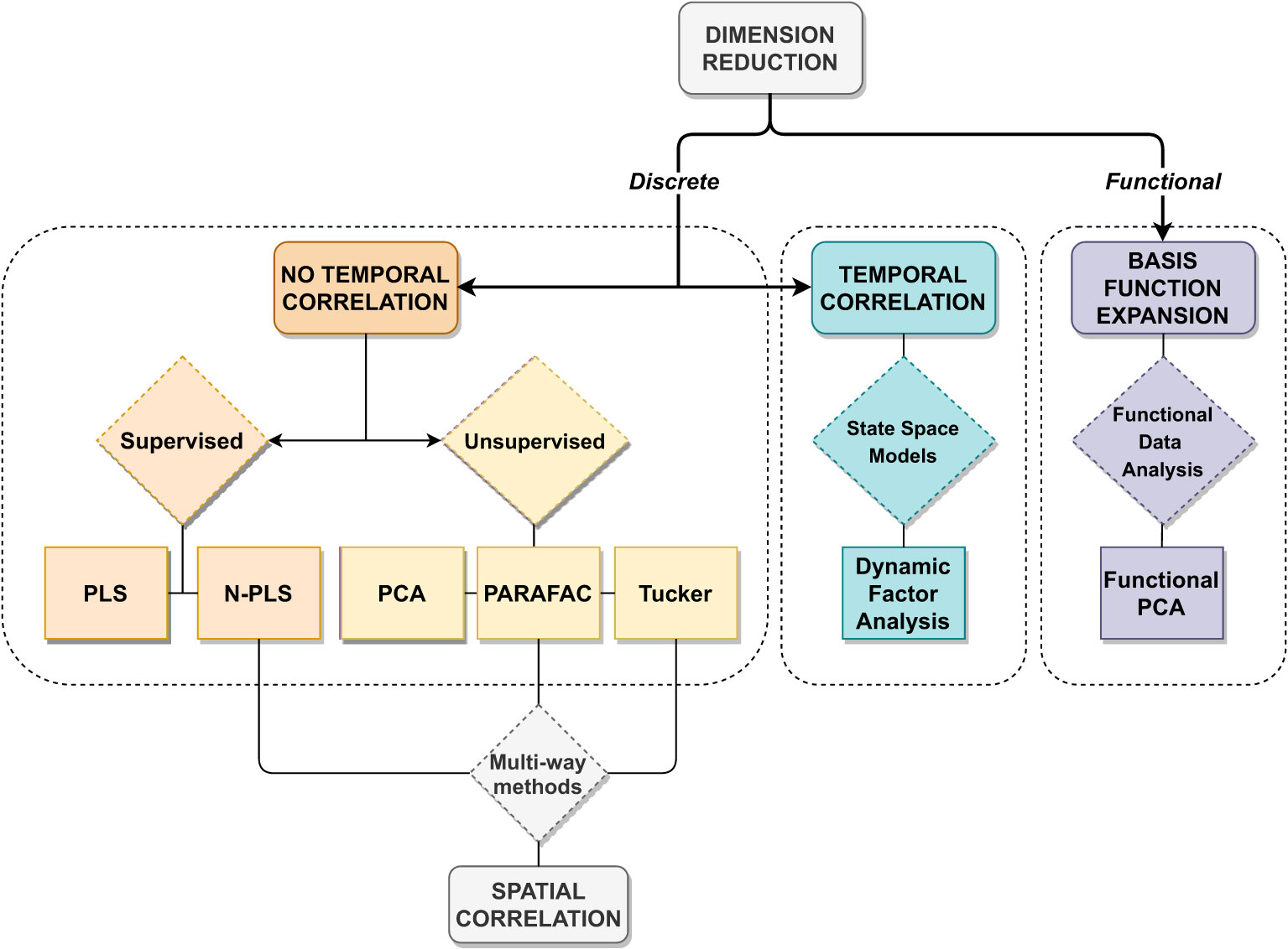
Figure 1 Overview of the applied statistical techniques for discrete-time and functional data, including temporal and spatial correlation.

2.1. Dataset

Our study is based on data from various numerical models (see Figure 2): a coastal water quality model, a numerical weather prediction model, and a climate model. The ecological indicator variable is chlorophyll-a concentration, a proxy for algal biomass, while the atmospheric variables are air temperature, solar radiation, eastern and northern wind components, air pressure, relative humidity, and total cloud cover. These are standard atmospheric variables simulated by most modelling systems for both operational purposes and climate experiments.

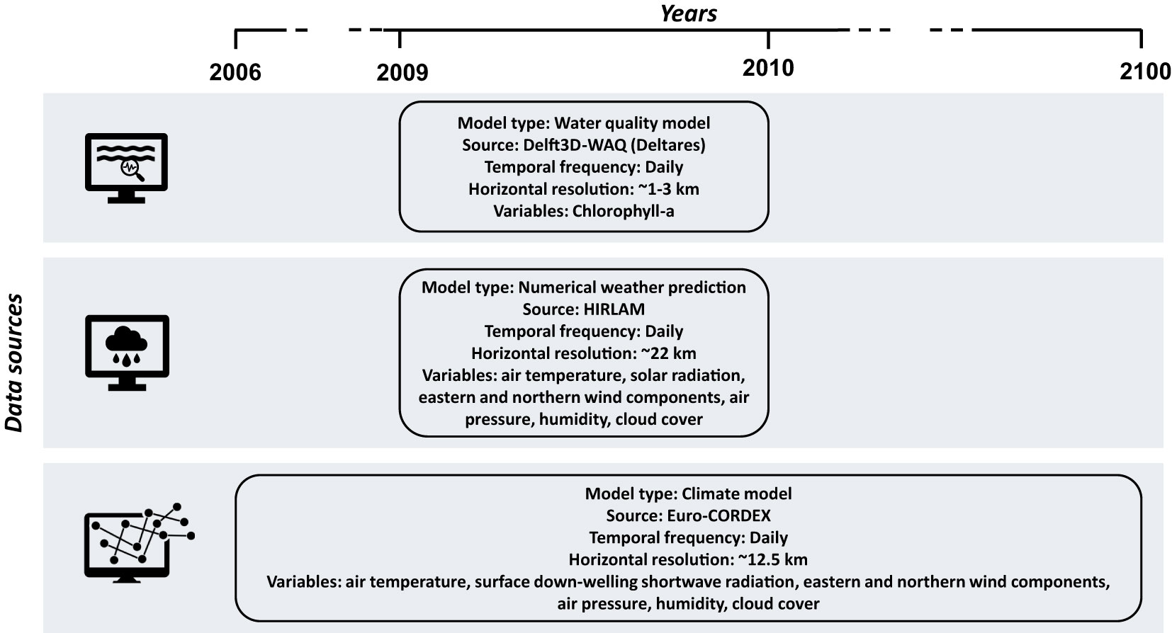
Figure 2 Overview of the data used in the study (model type, source, temporal frequency and variables) for the marine water quality model (top), numerical weather prediction model (middle), and climate model (bottom).

2.1.1. Chlorophyll-a concentration data

The chlorophyll-a concentration data is obtained from the water quality sub-module of the Delft3D integrated modelling system, Delft3D-WAQ (https://www.deltares.nl/en/software/158delft3d-4-suite/) (Blauw et al., 2009). In this research an existing model setup is used, which has been previously calibrated and validated for the location of our study area (Los et al., 2008). The spatial domain of the physical model covers the Southern North Sea with coarser horizontal resolution offshore and finer resolution along the Dutch coast, as shown in Figure 3. The model comprises of twelve vertical layers, making it a three dimensional physical model. The horizontal resolution of the water quality model in the Dutch Wadden Sea ranges from 1-by-2 km to 2.5-by-3 km on a curvilinear grid.

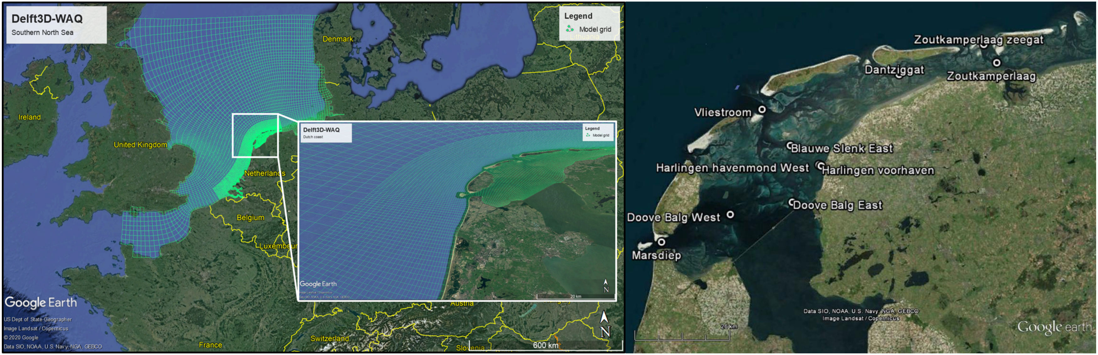
Figure 3 Case study area: Dutch Wadden Sea. Delft3D-WAQ model domain in the Southern North Sea and along the Dutch coast (left panel, source: (Mészáros et al., 2021)). Location of the stations where time series data was extracted (right panel).

Delft3D-WAQ is a comprehensive hybrid ecological model including an array of modules reproducing water quality processes that are then combined with a transport module to calculate advection and dispersion. The model most importantly calculates primary production and chlorophyll-a concentration while integrating dynamic process modules for dissolved oxygen, nutrient availability and phytoplankton species. This Delft3D-WAQ setup includes the phytoplankton module (BLOOM) that simulates the growth, respiration and mortality of phytoplankton. Using this module the species competition and their adaptation to limiting nutrients or light are simulated (Los et al., 2008).

2.1.2. Atmospheric data

Two sources of atmospheric data are used in this study: (1) outputs of an operational numerical weather prediction model, and (2) results of a regional climate modelling experiment. First, the High Resolution Limited Area Model (HIRLAM) model (Meijgaard et al., 2008) output is used, which was applied as atmospheric forcing for the Delft3D-WAQ model setup to compute chlorophyll-a concentration. HIRLAM is a Numerical Weather Prediction (NWP) system developed by the international HIRLAM programme (http://hirlam.org/) (Undén et al., 2002). Since it is the Delft3D-WAQ input data that drives the processes, it allows the exploration of the correlations between atmospheric forcing and numerically computed ecological response. The data for this study are obtained from the 22 km grid resolution HIRLAM model and include near-surface air temperature, solar radiation, eastern and northern near-surface wind components, surface pressure, near-surface relative humidity, and total cloud cover. All HIRLAM model output variables were used in the Delft3D-WAQ model as temporally and spatially variable forcing fields except solar radiation, which is an area average, therefore the same for the entire domain.

Additionally, simulated values of climate variables are acquired from the high resolution 0.11 degree (∼12.5 km) EURO-CORDEX Coordinated Regional Downscaling Experiment (https://www.euro-cordex.net/) (Jacob et al., 2014), which uses the Swedish Meteorological and Hydrological Institute Rossby Centre regional atmospheric model (SMHI-RCA4) (Samuelsson et al., 2015). In order to produce various regionally downscaled scenarios, EURO-CORDEX applies a range of General Circulation Models (GCMs) to drive the above mentioned Regional Climate Model (RCM). The four driving GCMs in this study are the National Centre for Meteorological Research general circulation model (CNRM-CM5) (Voldoire et al., 2013), the global climate model system from the European EC-Earth consortium (EC-EARTH) (Hazeleger et al., 2012), the Institut Pierre Simon Laplace Climate Model at medium resolution (IPSL-CM5A-MR) (Dufresne et al., 2013), and the Max-Planck-Institute Earth System Model at base resolution (MPI-ESM-LR) (Giorgetta et al., 2013). In addition to the driving models, further scenarios are obtained by considering different socio-economic changes described in the Representative Concentration Pathways (RCPs). RCPs are labeled according to their specific radiative forcing pathway in 2100 relative to pre-industrial values. This study includes RCP8.5 (high), and RCP4.5 (medium-low) (van Vuuren et al., 2011) and four driving GCMs for the projection period between 2006-2100. Together the four different driving GCMs and two RCPs provide us with an ensemble of eight trajectories per climate variable. The climate variables included in the analysis are near-surface air temperature, surface downwelling shortwave radiation, eastern and northern near-surface wind components, surface pressure, near-surface relative humidity, and total cloud cover. For this dataset, near-surface means at a height between 1.5 to 10.0 m.

2.1.3. Data processing

The above introduced datasets are temporally varying multivariate fields covering large domains (see Figure 4). For the purpose of this study, time series data were extracted at ten locations of Rijkswaterstaat monitoring stations in the Dutch Wadden Sea (see Figure 3). Both the atmospheric variables and the chlorophyll-a concentration were provided as 6-hourly datasets. The longer and higher frequency data were sub-sampled to the period between 1st of March and 1st of November, daily at 12:00 (245 time steps). The model simulation year (2009) was chosen based on the fact that a detailed study was conducted (at Deltares) for that year with high resolution information on the suspended matter fields which are crucial for water quality computation in the shallow Wadden Sea. The reason for selecting a reduced time period (9 months) is to concentrate on the season of high phytoplankton productivity and to eliminate near zero chlorophyll-a values during winter. Moreover, the daily time step at 12:00 was selected to eliminate zero radiation values during the night. All variables were then centered to their mean and divided by their standard deviation to eliminate the problem of different measurement units. Finally, the right skewed chlorophyll-a concentration was log transformed to achieve a more symmetrical distribution that may improve the performance of statistical models used in the study. It is a standard practice to log transform chlorophyll-a as it is approximately lognormally distributed in marine waters (Campbell, 1995). The distribution of chlorophyll-a concentration (all locations and all time steps) before and after log transformation are shown in Figure S1 (Supplementary Material). The pair plot of all variables with kernel density estimation is displayed in Figure S2 (Supplementary Material).

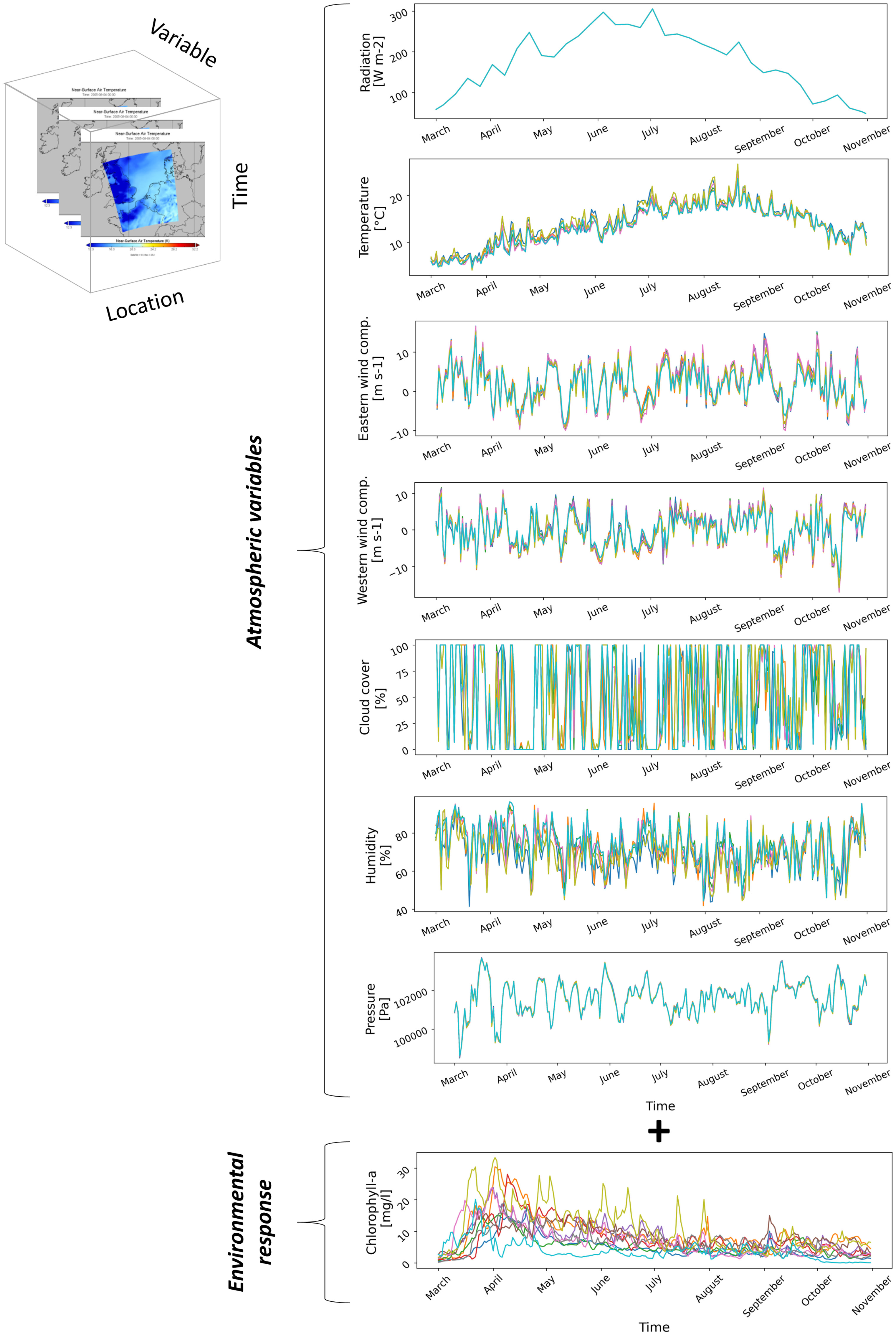
Figure 4 Illustration of the atmospheric and environmental variables used in the study.

Figure 5 shows the Spearman’s rank correlation coefficient of all variables after scaling (data taken from all stations). The same plot using Pearson correlation coefficient can be found in Figure S3 (Supplementary Material). It can be observed that solar radiation and air temperature have the highest correlation with chlorophyll-a. Moreover, cross-correlation between the atmospheric data an also be identified, e.g. pressure and northern wind component or humidity and air temperature. It is important to note that while air temperature and solar radiation are positively correlated, they have different impact on chlorophyll-a concentration: air temperature has negative correlation, whereas solar radiation has positive correlation with chlorophyll-a. Since in the North Sea the correlation between solar radiation/air temperature and chlorophyll-a concentration highly depends on the region (offshore or coastal) and the temporal scales (short, seasonal, long) there could be various reasons. In our case, it might be attributed to the phenomena reported by Blauw et al. (2018), who found that the thermal mixing of phytoplankton cells (from the deep chlorophyll maximum) into the surface layer is the dominant process explaining the negative correlation between sea surface temperature and the chlorophyll concentration in the daily time series (in the Southern North Sea).

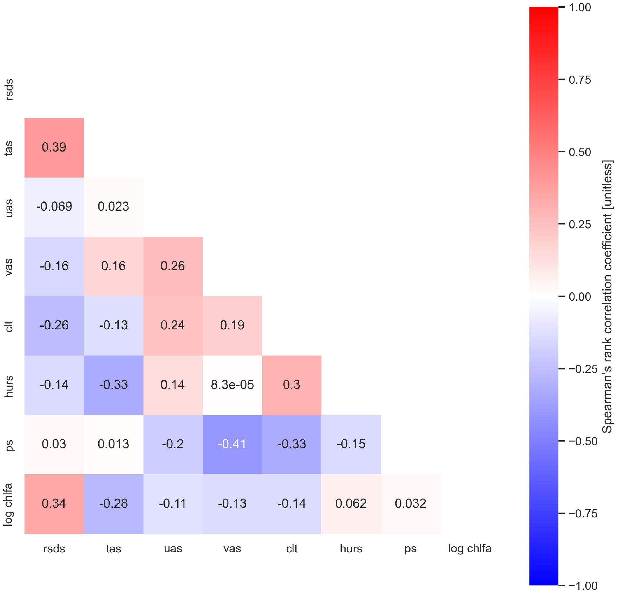
Figure 5 Heatmap with Spearman’s rank correlation coefficient. Dark red indicates strong positive, while dark blue indicates strong negative correlations. Data from all time series. Abbreviations: solar radiation (rsds), air temperature (tas), eastern (uas) and northern (vas) wind components, cloud cover (clt), humidity (hurs), air pressure (ps), chlorophyll-a (chlfa).

2.2. Two-way and multi-way methods

2.2.1. From PCA to N-PLS

This section briefly introduces the steps to extend the two-way component methods to multi-way regression methods. For convenience, Principal Component Analysis (PCA), Principal Component Regression (PCR) and ordinary PLS regression are introduced briefly, because the N-PLS regression is based on these algorithms. Assuming that X∈ℝ^I×J and $\underset{\_}{y}\in {ℝ}^I$ are column centred and scaled matrices, the predictor matrix X and response $\underset{\_}{y}$ are decomposed as follows:

where T is a matrix of scores (T=XP); P^′ is a matrix of X loadings, q is a matrix of $\underset{\_}{y}$ loadings, whereas E_X and e_y are the residuals. PCA focuses only on the predictor matrix projecting each data point onto the principal components while preserving as much of the data’s variation as possible. PCA finds R components such that they maximize the variance of the projected data in X. The description below is written for R=1. To calculate the 1^st PCA component, ${\widehat{x}}_{ij}$ is approximated with t_i core and w_j loading:

where $\underset{\_}{t}\in {ℝ}^I,\underset{\_}{w}\in {ℝ}^J,i\in \left\{1,\dots ,I\right\},j\in \left\{1,\dots ,J\right\}$, and ||w||=1. Then the score vector and loading vector can be obtained as follows:

Then the approximation of $\widehat{X}$ can be rewritten as:

with $T=\underset{\_}{t}$ and $P^{\prime }=\underset{\_}{w}$. Finally, the decomposition of X (for the 1^st PC situation) is obtained as:

The PCR algorithm is similar to the PCA algorithm except that it is extended with response y using Eq (2). In other words, PCR constructs R components the same way as PCA, but adds a regression step to it. Consequently, the regression coefficient $\underset{\_}{q}$ is obtained from regressing $\underset{\_}{y}$ on T

The PLS regression differs from PCR, due to its supervised nature, as it finds R omponents from both X and $\underset{\_}{y}$ such that covariance between the score vector t(w) and $\underset{\_}{y}$ is maximized:

Again, rewrite the approximation as Eq (7). with $T=\underset{\_}{t}$ and $P=\underset{\_}{w}$. Then obtain the decomposition as in Eq (8). Subsequently from Eq (2). the regression coefficient $\underset{\_}{q}$ is obtained as in Eq (9). As a consequence, PLS finds loading w that leads to a least squares solution to Eq (3). Moreover, the PLS score vector has maximal covariance with $\underset{\_}{y}$. In general, both PCA and PLS achieve dimension reduction by converting highly correlated variables to a set of uncorrelated variables through linear transformation. The difference is that PCA, as an unsupervised technique, captures maximum variance only in the predictor matrix without considering how each predictive variable may be related to the response variable. On the other hand, PLS combines information about the variances of both the predictors and the responses, while also considering the correlations among them (supervised dimension reduction). PLS is considered useful in particular if there are more independent (predictor) variables than dependent (response) variables, and if there is multi-colinearity in the predictors. Since in this study several correlated atmospheric variables are used to estimate one ecological response variable, the use of supervised dimension reduction techniques is preferable.

The N-PLS regression algorithm is an extension of the PLS regression algorithm to multi-way data, where essentially the bilinear model of X is replaced with a multilinear model of X. In case the data is three-way, as in this study, then an appropriate model of X is a trilinear decomposition, as depicted in Eq (16). The model of x_ij in ordinary PLS is shown in Eq (3), whereas in three-way PLS the approximation of x_ijk is given by the following equation:

where $\underset{\_}{t}\in {ℝ}^I,{\underset{\_}{w}}^J\in {ℝ}^J,{\underset{\_}{w}}^K\in {ℝ}^K$. In this case the three-way decomposition is defined by:

where ||w^J||=1 and ||w^K||=1. The regression coefficient $\underset{\_}{q}$ s obtained by regressing $\underset{\_}{y}$ on T as in Eq (9), rewriting the approximation as above in Eq (7). with T=[t] and P=[w] subsequently obtaining the decomposition as in Eq (8). Similar to ordinary PLS the resulting score vector has maximal covariance with $\underset{\_}{y}$ and the loadings $(w_j^J$ and $w_k^K)$ lead to a least square solution. For R>1 further components can be obtained as follows. Rewrite Eq (7) with $T=\left[\underset{\_}{t_1},\dots ,\underset{\_}{t_R}\right]$, $P=\left[\underset{\_}{w_1},\dots ,\underset{\_}{w_R}\right]$. Finally, decomposition of X is in Eq (8), and subsequently from Eq (2). the regression coefficient $\underset{\_}{q}$ is obtained as in Eq (9).

In summary, the N-PLS model first extracts the important features from the predictor dataset into the loading array P then estimates the regression coefficient vector $\underset{\_}{q}$ using least squares. For a more detailed description of the N-PLS algorithm the reader is referred to (de Jong, 1998; Bro, 1996; Smilde, 1997; Bro, 1998; Bro et al., 2001; Smilde et al., 2004).

2.2.2 Comparison of multi-way methods

Atmospheric datasets are often multi-dimensional due to the fact that they contain several variables, which are not only varying over time but also over space. Moreover, often additional dimensions are present such as different climate projection scenarios, or model ensembles, which simulate the same information but use different assumptions or initial conditions. Three-way data that contain information on different variables, over time and space can be organized in a three-way array $\underset{\_}{X}=X_{i,j,k}$. In our case the first dimension (mode 1 or index i of the three-way array $\underset{\_}{X}$ corresponds to time, the second dimension (mode 2 or index j corresponds to different atmospheric variables, and the third dimension (mode 3 or index k corresponds to location. Consequently, each frontal slice X_k represents a location with variables j sampled over time i.

The distinction between component and regression models should also be noted. The typical purpose of component models on one block of data is exploring the patterns and interrelations using latent variables (principal components), while regression models are aimed at predicting a block of data (response) using another block of data (predictors) through a prediction model. Consequently, component models require one block data, while regression models need multi block data. The above mentioned dimension reduction methods (PCA and PLS) are two-way component and regression models that cannot be directly applied to multi-way data. The traditional approach to deal with multi-way data is to use unfold methods (sliced analysis) such as the one introduced by Wold et al. (1987). Unfold methods first unfold the multi-way array to a two-way matrix and then perform ordinary PCA and PLS analysis. However, as Bro (1996) has pointed out, the unfolding methods are not favourable since they do not make use of the multi-way structure in the data, they are often complex (using many parameters) and more difficult to interpret compared to the multi-way methods that do not use unfolding.

More appropriate models have been developed for handling multi-way data, which are the so-called multi-way component and regression models, schematized in Figure 6. Multi-way component models are basically generalizations of the two-way solutions to higher order arrays. One generalization of PCA to higher orders is Parallel factor analysis (PARAFAC), also known as trilinear decomposition, with general equation given by:

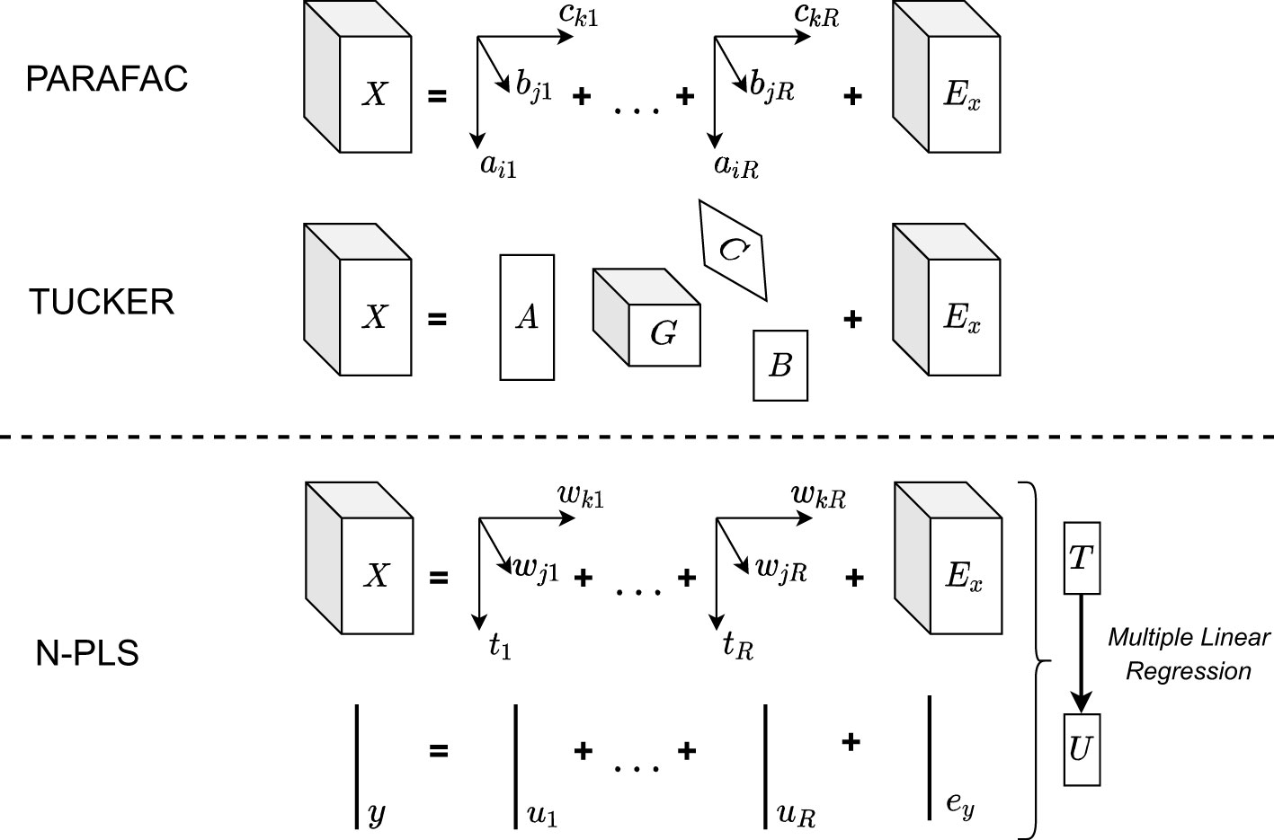
Figure 6 Schematization of multi-way models. The cubes (cuboids) represent three dimensional arrays (X denoting the data array, G the core-array for the Tucker model and Ex the residual array for all models), the three arrows represent orthogonal vectors (trilinear factors a1, b1, c1, and loading vectors wk, wj with score vector t), while the lines represent vectors (response vector y, score vector u, and residual vector ey), and the rectangles represent loading matrices for the Tucker model (A, B, C). Adopted from (Fujiwara and Mohr, 2009).

where R is the number of components used to fit the model; a_ir,b_jr,c_kr are ‘triads’ (trilinear factors) and e_ijk is the residual (see Figure 6). Note that here R>1 s explicitly possible, compare PCA and PLS descriptions above. Another generalization is the Tucker decomposition, also called N-mode Principal Component Analysis (Bro, 1997). For the three-way case, Smilde et al. (2004) describe the Tucker3 model with the following equation:

where a_ip,b_jq,c_kr are elements of the loading matrices A, B, C, g_pqr is an element of the core-array G nd e_ijk is the residual element in E as depicted in Figure 6.

Similarly, the two-way partial least squares regression was also extended to multi-way data as described in Section 3.2.1. The N-way Partial Least Squares (N-PLS) method was developed by (Bro, 1996) and further elaborated by (de Jong, 1998; Smilde, 1997; Bro, 1998; Bro et al., 2001). A pictorial representation of N-PLS model is shown in Figure 6. Due to its desirable properties, as compared to the unfolding methods, the N-PLS method has been applied in a range of areas such as chemometrics, neuroscience and environmental analysis (Bro, 2006), food industry (Favilla et al., 2013), organic pollutants in the environment (Mas et al., 2010) or most recently in agriculture (Lopez-Fornieles et al., 2022).

Moreover, recently another generalized multilinear regression method, the Higher Order Partial Least Squares (HOPLS), was introduced by (Zhao et al., 2013). HOPLS differs substantially from N-PLS in that it uses the Tucker tensor decomposition (see Eq. (17)) instead of the trilinear decomposition (see Eq. (16)), hence, it benefits from the advantages of Tucker over PARAFAC. Zhao et al. (2013) found that HOPLS could outperform N-PLS and PLS in case of small sample sizes and higher order N>3 response data $\underset{\_}{y}$. While HOPLS appears to be a promising method in those cases, it should be noted that in this study sufficient number of samples is available and the response $\underset{\_}{y}$ dataset is not high dimensional N≤3 The substantial differences between the above mentioned multi-way methods can be seen from their schematic representation (Figure 6). A comprehensive review of other dimension reduction methods for multidimensional data via Multilinear Subspace Learning (MSL) can be found in (Lu et al., 2013). In this study the PCA, PLS, PARAFAC and Tucker algorithms were implemented using open source Python packages such as scikit-learn and TensoLy, whereas for the N-PLS algorithm the N-way Toolbox (Andersson et al., 2000) was used in Matlab.

In order to showcase the differences between the various two-way (PCA, PLS) and multi-way (PARAFAC, TUCKER, N-PLS) dimension reduction methods, they were applied on the atmospheric and environmental data (from Section 2.1) for prediction. Their prediction errors were analysed from 10-fold cross-validation. K-fold cross-validation, briefly described in (Hastie et al., 2009), uses a subset of the available data as a training set to fit the model and a different subset as a test set, where the full dataset is split into K qual-sized parts, in this case K=10. For the prediction of every k−th subset the model is fitted to the remaining K−1 subsets of the data and the prediction error of the fitted model is calculated. This process is repeated for k=1,2,…,K and the K estimates of prediction error are averaged. First the Mean Squared Error (MSE) with only the intercept (no principal components in regression) was calculated, and later on the MSE is computed using 10-fold cross-validation for the principal components, adding one component at the time in increasing order. The error measures of the unsupervised methods were obtained by extracting their computed model factors (with different number of components) which were then used to fit linear regression. The results of estimated mean squared errors of predicting y from 10-fold cross-validation are shown in Figure 7.

Figure 7 Comparison of two-way (point markers) and multi-way (triangle markers), unsupervised (PCA, PARAFAC, TUCKER) and supervised (PLS, N-PLS) dimension reduction models. Prediction errors (MSE) from 10-fold cross-validation with increasing number of components. Prediction is done at Marsdiep Noord station.

Apart from the prediction accuracy, it is also investigated how strongly each component (latent variable) in the two component N-PLS model (the best performing multi-way model) depends on the original variables (see Figure 8).

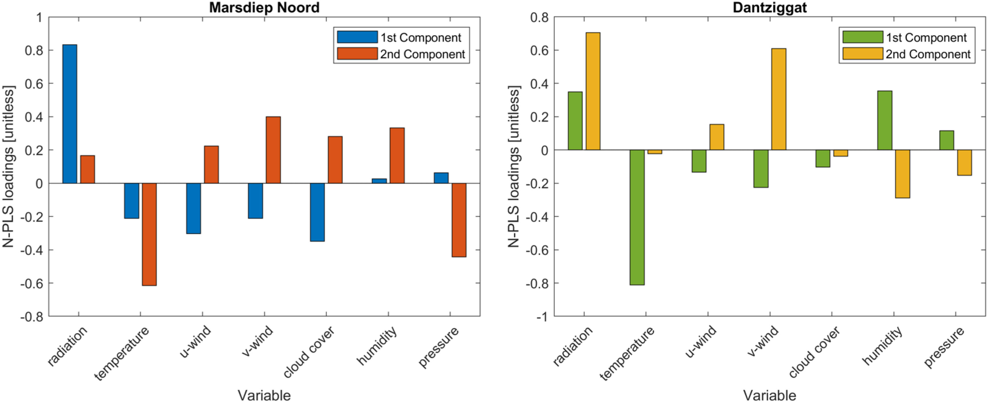
Figure 8 Importance of predictor variables in the N-PLS model. Loadings of atmospheric variables in the 1st and 2nd N-PLS components for locations Mardiep Noord (left) and Dantziggat (right). Eastern and northern wind components are denoted by u-wind and v-wind, respectively.

2.3. Dynamic factor analysis

The previously presented dimension reduction techniques are able to identify unobserved factors that influence a substantial portion of the variation in a larger number of observed variables, and able to summarize the dataset through decomposition. None of these techniques, however, is designed for time series analysis as temporal correlation is neglected. Dynamic Factor Analysis (DFA) is a factor model that explicitly models the transition dynamics of the unobserved factors; hence, it is a dimension reduction technique that is designed for time series data. In fact, DFA is a multivariate time-series analysis technique that estimates underlying common trends in multivariate time series (Harvey, 1990; Mike West, 1997; Lütkepohl, 2005). The time series are modelled using a linear combination of common trends, explanatory variables, and a noise component (Zuur et al., 2003a).

Given N ime series, these could be analysed by univariate models by treating them as N separate univariate time series. However, this would result in N estimated trends without considering the interactions between them. DFA aims to overcome this disadvantage by reducing the N univariate trends to M common trends, where 1≤M<N. The main objectives of DFA on environmental time series are therefore identifying underlying common trends (unobserved factors) in the input time series, identifying interactions between the time series, and analysing the effects of explanatory variables.

The basic concept of DFA is to decompose the multivariate data into trends, explanatory variables and noise. Supposing that y_t is a univariate response variable measured in time t where t=1,…,T one of the simplest univariate time series models is given as follows:

where α_t represents the factor (unknown trend) at time t while ∈_t and η_t are error components (noise). This model is called the random walk trend plus noise model. A formulation for the DFA with N time series (N rows) and M common trends (M columns) can be written as:

or in generic form:

where Γ is a factor loading matrix with dimension N×M and contains the unknown factor loadings, which are multiplication factors that determine the linear combination of the original variables; and α_t is a vector of the M common trends at time t with dimension M×1. It is generally assumed that the error terms are independent, normally distributed with mean 0 and an unknown diagonal or symmetric/non-diagonal covariance matrix: ∈_t∼N(0,H) η∼N(0,Q) and α₀∼N(α₀,V₀) where H,Q,V₀ are covariance matrices (Zuur et al., 2003b). Based on these parameters the covariance matrix of y_t can be written as:

In order to include K explanatory variables in the DFA, equations (22)– (23) can be extended to the following model:

where D is an N×K matrix containing the partial (standardized) regression coefficients, and x_t is a K×1 vector containing the values of the K explanatory variables at time t. The effects of explanatory variables are modelled as in linear regression, and therefore it depends on the same underlying assumptions, such as normality, independence, and homogeneity of residuals (Zuur et al., 2003a).

Equations (25)- (26) can be cast into state space form, and the unknown trends can be estimated via the Kalman filter. The likelihood is then evaluated based on the filtering recursions, and maximum likelihood estimation is used to estimate the parameters. The Kalman Filter and smoother algorithm for the model in equations (25)- (26) can be found in (Zuur et al., 2003b).

The dynamic factor model was applied to the ten chlorophyll-a time series. The main objective was to identify underlying common trends and further analyse the effects of atmospheric variables on chlorophyll-a concentrations, this time considering temporal correlation. Since standard dynamic factor models are not designed for multi-way data, such as N-PLS, the atmospheric data is averaged over the locations. In order to verify that the underlying assumptions of the dynamic factor model are not violated, several tests were conducted. These tests include plotting the standardized residuals over time, checking the normality of the residuals and plotting the correlogram (see Figure S4 in the Supplementary Material). It was verified that residuals are uncorrelated (since the autocorrelations are near zero of all time-lag separations), and normally distributed with mean zero. Thus, underlying assumptions are valid.

2.4. Functional PCA

So far the paper has investigated the features and relationships between short term (1 year long) meteorological data and environmental response. These datasets offered us the opportunity to apply supervised techniques since the environmental response was computed with the meteorological data as input. Moreover, we could consider temporal dependence and compute unobserved factors in the time series due to the reasonable number of time steps that allow us to apply computationally intensive state space models. However, apart from the analysis on short term data, we are also interested in investigating the features of the long term (climate scale) atmospheric projections and potential for data reduction. In order to achieve this, firstly we use Euro-CORDEX climate projections (covering the entire 21^st century) instead of numerical weather prediction model outputs. Secondly, we analyse the discretely computed (in time) atmospheric data in the functional data space. This allows us to apply functional data analysis and study functional variation, which is more logical for climate projections that are long time series of modelled variables and are not meant to study short term changes and daily variability. Naturally, an interesting feature of the climate projections is their long term trends. Conclusions on their seasonal variability and the similarities between climate scenarios are less often drawn, however. We aim to reach such conclusions through Functional Data Analysis. By treating these long term climate projections as functional data our objective is to find an underlying function that can characterize the general shape of the time series, explain their variability (functional variation), reduce data complexity, and to aid the interpretation of the underlying variability sources (Ramsay and Silverman, 2005). The findings of the previous analyses and the Functional Data Analysis can be jointly used for climate impact assessment by aiding the atmospheric variables selection for studying chlorophyll-a climate response, as well as the identification of important features of the climate projections for further statistical models.

Functional data representation is commonly done by smoothing the discrete-time data with basis expansion (e.g. constant, polynomial, polygonal, B-splines, power, exponential, Fourier) as a pre-processing step. In our study, a Fourier basis expansion is applied, which has good computational properties especially when the data points are equally spaced. Moreover, Fourier bases are natural for describing periodic data, such as atmospheric variables, and therefore it is commonly used in this domain. The functional basis components can be then estimated through Functional Principal Component Analysis (FPCA).

The underlying idea is that a function x_i(t) can be expressed as a basis expansion:

And

where $\overline{x}$(t) is the functional mean (zero if the data is mean centered), φ_j(t) are the orthonormal eigenfunctions and f_ij are the Functional Principal Component Scores. The first few eigenfunctions and eigenvalues can be used for data reduction and feature extraction, while the Functional Principal Component Scores can be used to describe, cluster and classify the curves (Segovia-Gonzalez et al., 2009). The Functional Principal component analysis in this research uses an open source Matlab toolbox (Ramsay et al., 2009).

While the other above mentioned methods (multi-way methods and dynamic factor model) are used for identifying the most important atmospheric variables affecting chlorophyll-a concentrations in a shorter time interval, in this research Functional Principal Component Analysis is used to investigate different features of the long term climate projections spanning the 21^st entury (from 2006 to 2100). Functional Principal Component Analysis was therefore applied to the Euro-CORDEX climate projections to compare the functional variation of climate variables, and to describe, cluster and classify the climate scenarios for the two most important variables (radiation and temperature).

The discrete-time data points are first transformed to functional data using a Fourier basis expansion. The left panel of Figure 9 shows the atmospheric variables as functional data for an arbitrarily selected year within the 95 year interval. The well distinguishable sinusoidal shapes of solar radiation and temperature can be seen in the figure. Functional Principal Component Analysis with two principal components is then performed on the functional data and the scores of the first two components are plotted to analyse similarities between the variables (right panel of Figure 9). Moreover, as a second experiment, using Functional Principal Component Analysis the aim is to classify and cluster the climate scenarios (Representative Concentration Pathways and driving General Circulation Models) for the two important climate variables (radiation and temperature), see Figures 10, 11.

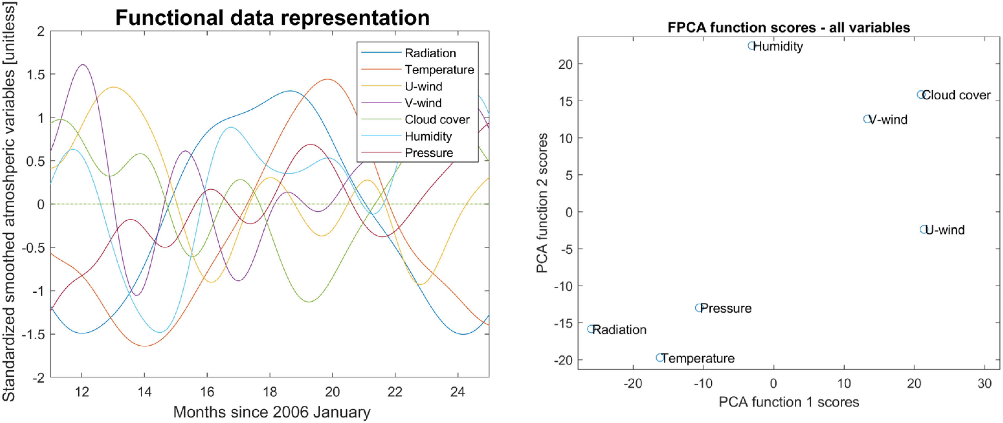
Figure 9 Functional Principal Component scores for the Euro-CORDEX climate variables. Atmospheric variables transformed to functional data (for an arbitrarily selected year) on the left panel, and clustering of variables based on the FPCA function scores on the right panel.

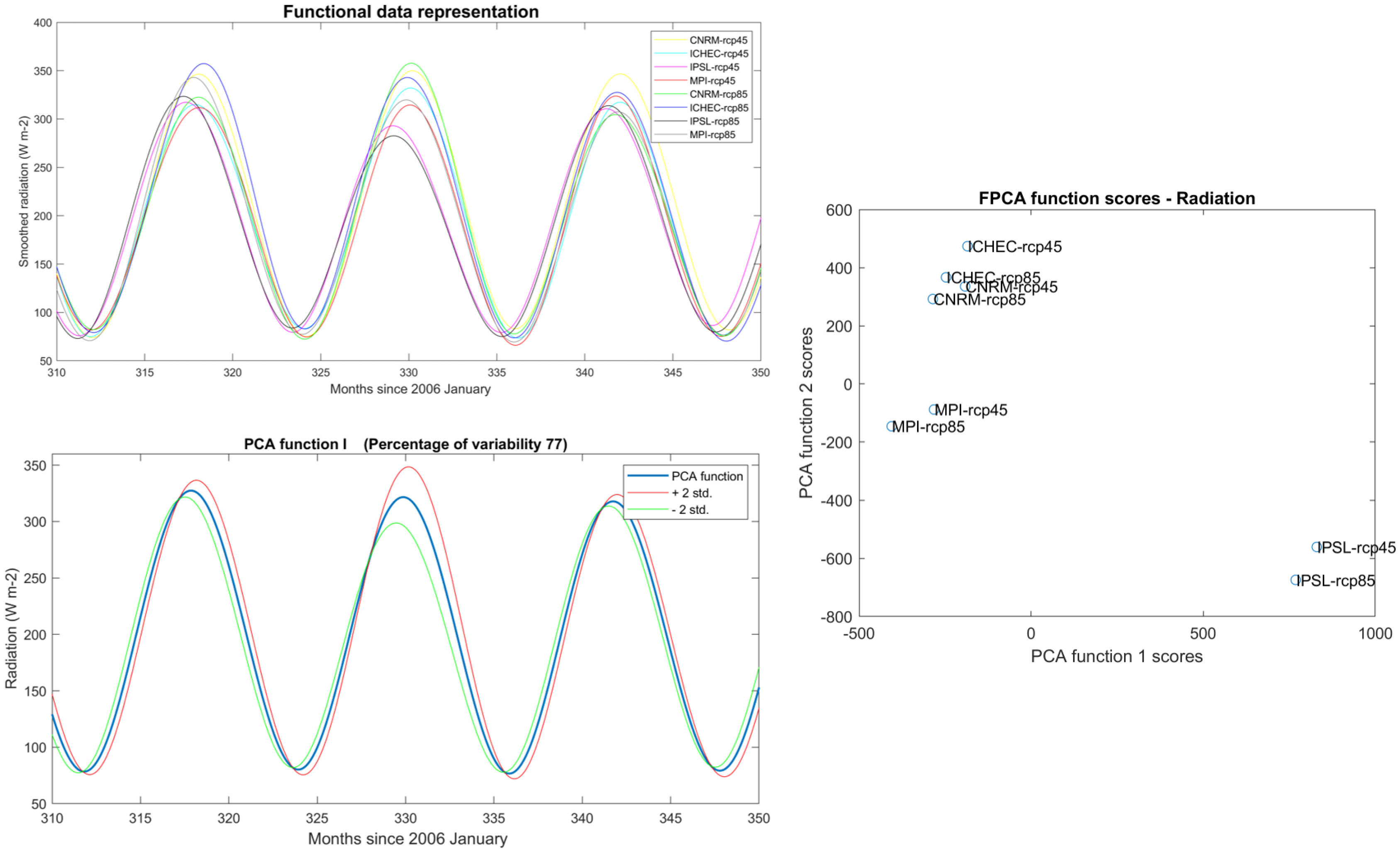
Figure 10 Functional Principal Component Analysis for the Euro-CORDEX solar radiation scenarios. Eight solar radiation scenarios transformed to functional data on the upper left panel, the first PCA component with ± two standard deviations on the bottom left panel, and clustering of scenarios based on the PCA function scores on the right panel.

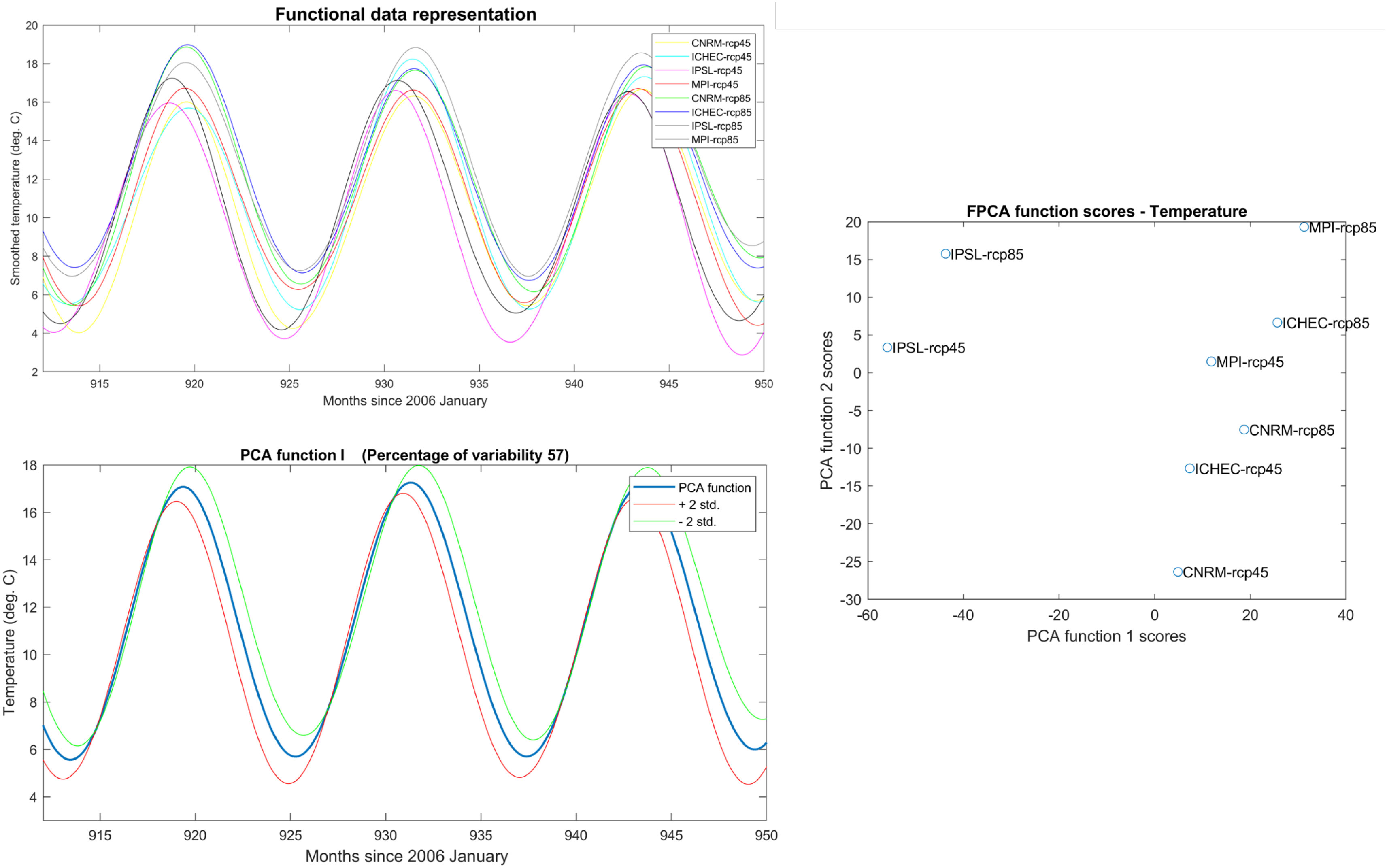
Figure 11 Functional Principal Component Analysis for Euro-CORDEX air temperature scenarios. Eight air temperature scenarios transformed to functional data on the upper left panel, the first PCA component with ± two standard deviations on the bottom left panel, and clustering of scenarios based on the PCA function scores on the right panel.

3. Results

3.1. Comparing two-way and multi-way methods

Another observation is the performance difference between PCA, PARAFAC and Tucker models. Both PARAFAC and TUCKER are generalizations of PCA to a higher order, with the important difference that the PARAFAC model has the attractive feature of providing unique solutions (there is no problem with rotational freedom). If the data are approximately trilinear, the true underlying phenomena can be found if the right number of components is used and the signal-to-noise ratio is appropriate (Bro, 1998). The Tucker model is, however, more flexible and has rotational freedom. It is not structurally unique as PARAFAC. This makes the Tucker model complex and might explain why it has lower performance for this specific example. A restricted Tucker model version exists where domain knowledge is used to restrict the core elements, forcing individual elements to take specific values. This way it is possible to define models that uniquely estimate certain properties. This could be seen as a structural model tailored to a specific problem. In this paper restricted Tucker models were not used.

In Figure 8 the loadings of the first two components of the N-PLS model (the best performing multi-way model) are given for two different locations. By identifying the original predictor variables that weight most heavily one can draw conclusions on the underlying physical processes. Moreover, less important predictors could be excluded from the dataset in order to reduce the number of variables. In Figure 8 it can be observed that at Marsdiep Noord, a location of a deeper tidal inlet, the highest loadings are given to radiation in the first component and to temperature in the second component. On the other hand, at Dantziggat, located in the shallow inter-tidal area, the opposite can be observed: the highest loadings are given to temperature in the first component and to radiation in the second component. Moreover, apart from temperature and radiation which have the highest loadings, northward-wind also has high loading in the second component at Datziggat. The factor loadings indicate the differences in the physical systems between the two locations. In deeper areas (Marsdiep Noord) solar radiation is the primary driver of the onset of phytoplankton blooms, while in shallower areas (Dantzigat) radiation intensity is slightly less limiting and light availability in the water column heavily depend on wind, which influences turbidity due to the mixing of layers and suspension. This could explain the greater importance of wind speed at Dantziggat, especially that northerly winds cause the highest surges of sea water along the Dutch coast (Klein Tank and Lenderink, 2009) that leads to enhanced mixing. In addition, thermal stratification and vertical mixing conditions are different at the two locations, Marsdiep Noord being intermittently stratified and Dantziggat being permanently mixed (van Leeuwen et al., 2015). This influences nutrient availability in the mixed layer depth as well as phytoplankton composition and therefore could be responsible for the greater importance of air temperature at Dantziggat. Moreover, top-down phytoplankton governing factors (e.g. grazing, filter-feeding) are also different at the two locations. For instance the density of filter-feeders is much higher near Dantziggat (Folmer et al., 2014).

3.2. Dynamic factors

Choosing the optimal number of unobserved factors is crucial to find a model that identifies common trends in the dataset without significant loss of statistical information. In order to find the optimal number of factors, the Akaike’s Information Criterion (AIC) for each model setup (different number of factors, error covariance matrix diagonal or unstructured) was calculated and the model containing the lowest AIC value was selected as optimal. The selected model contains two factors if the error covariance matrix is set to diagonal. The identified two unobserved factors can be seen in the middle panel of Figure 12. It should be noted that the second factor has negative factor loadings, and for demonstration purposes, it was plotted with negative sign. The results indicate two well distinguished trends. The first factor represents the trends of those locations where the chlorophyll-a concentration peak (spring bloom) occurs earlier, such as Dantziggat. This is confirmed by the factor loadings Γ. On the other hand, the second factor shows the pattern of the locations where the occurrence of the peak is delayed. The identified temporal shift between locations in the onset of the spring bloom can be explained by the different system dynamics of the areas, for instance shallower intertidal zones and the proximity from river or tidal inlets.

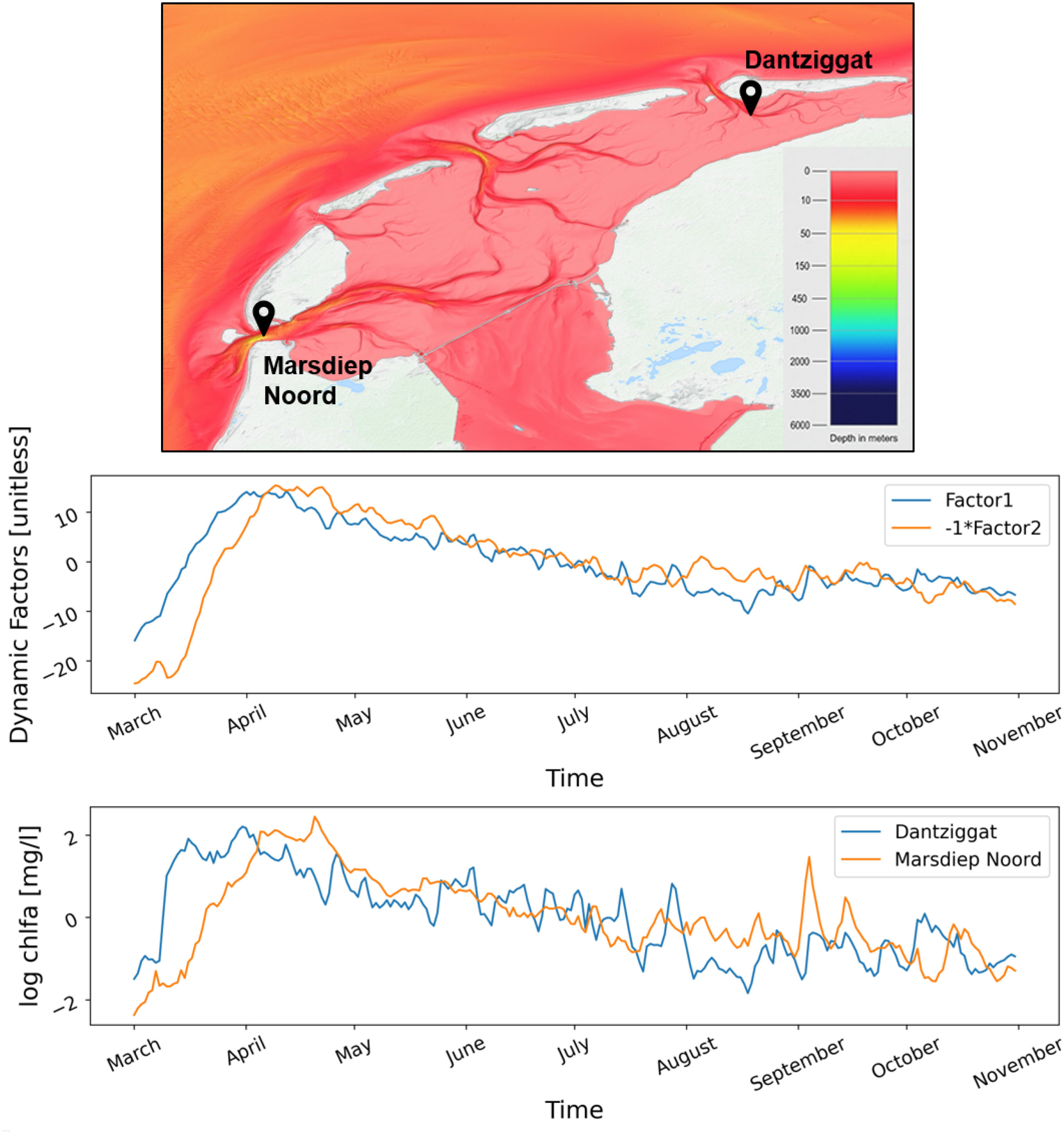
Figure 12 Underlying trends in chlorophyll-a time series. First and second factors of the Dynamic Factor model simulating chlorophyll-a trends with atmospheric variables as exogenous variables (middle). Log chlorophyll-a time series at representative stations (bottom). Bathymetry map showing the location of the representative stations (top). Map source is https://portal.emodnet-bathymetry.eu/.

The partial standardized regression coefficients of the dynamic factor model for the two representative stations Marsdiep Noord and Dantziggat (see Figure 13) are in agreement with the findings of N-PLS loadings and confirm that radiation and temperature are the most important atmospheric variables. It is also confirmed that at Dantziggat air temperature has significantly larger impact than at Marsdiep Noord. As mentioned above, this might be related to the differences in thermal stratification, mixing conditions and trophic interactions between the two locations. Nevertheless, considering temporal correlation the relative impact of solar radiation (compared to the other variables) seems to be even more important, especially at station Marsdiep Noord. This finding could be explained by the fact that phytoplankton biomass onset in this coastal ecosystem highly depends on the timing of increased energy from solar radiation during spring (Sommer and Lengfellner, 2008). In fact, it was reported by (Sommer and Lengfellner, 2008) that the (external) light regime appears to play a more important role in the initiation of spring blooms than temperature.

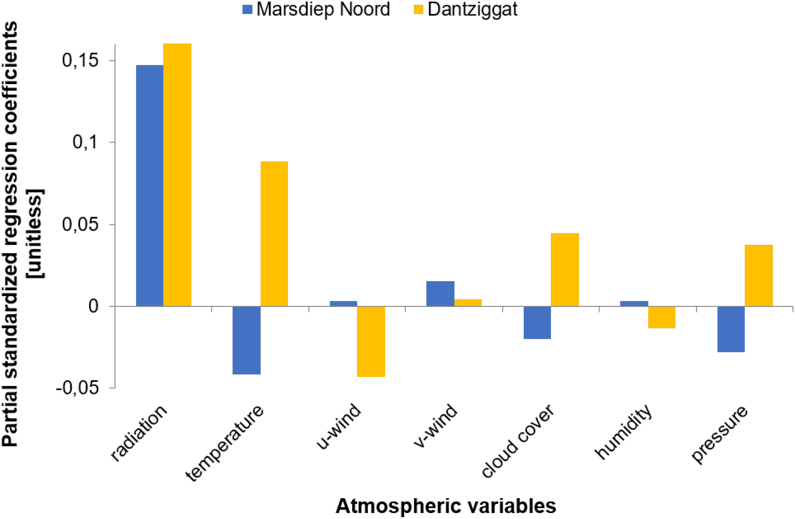
Figure 13 Dynamic Factor model partial standardized regression coefficients for Marsdiep Noord and Dantziggat stations demonstrating the effects of atmospheric variables as exogenous variables to model chlorophyll-a trends.

3.3. Functional principal components

An important aspect of FPCA is the examination of the scores of each curve (variable) on each component (here we display the first two). Figure 9 (right panel) shows the scores of the first two components of the Functional Principal Component Analysis applied to Euro-CORDEX climate variables. In order to draw conclusions from this figure, one must take into consideration the inverse correlation between two group of variables: cloud cover and northerly wind on one hand and radiation, temperature, and pressure on the other hand. These variables have relatively similar FPCA function scores but the scores of second group have negative signs (expressing the inverse correlation). Known examples are the anticorrelation of atmospheric pressure and cloud cover (high pressure meaning lower cloudiness), or cloud cover and solar radiation (high cloudiness meaning lower surface downward solar radiation).

After accounting for the sign of the FPCA scores, a single main cluster can be distinguished that group variables (their functional representations) with similar characteristics and two variables, eastern wind and humidity, that are relatively separated. In general the correlation between cloud cover and wind speed is documented (Essenwanger, 1962) but the reason for eastern wind to be separated could be explained by the fact that at this specific location the maritime air mass is mainly brought by the northerly wind from the North Sea to replace the dry continental air mass (Klein Tank and Lenderink, 2009) causing cloud formation. The fact that radiation and temperature are positively correlated and lie near each other is expected, due to their similar sinusoidal functional shapes. The relationship of variations in air temperature to changes in air pressure was also reported in literature (Aguilar and Brunet, 2001) based on the analysis of long historical records. They concluded that changes in atmospheric circulation (influenced by air pressure) has a key role in air temperature variation, acknowledging that the relationship is seasonally dependent and impacted by the regional topography. Indirect links between air pressure and solar radiation were also discovered by (Klein Tank and Lenderink, 2009). They argue that high pressure systems impact air quality, which in turn affects solar irradiance (Zhang et al., 2022; Yang et al., 2022; Gómez et al., 2023). However, as the considered data are outputs of a climate model, which does not include air quality processes, this could not have been captured in our dataset.

Considering the Functional Principal Component Analysis results for the removal of multi-collinearity, one could expect that using only radiation or temperature might be sufficient without significant loss of statistical information. For climate impact studies at this location it should be considered, however, that solar radiation and temperature display different long term trends in this region and influence the phytoplankton dynamics differently. Based on the Euro-CORDEX projections, long term trends of radiation is constant or slightly decreasing, whereas air temperature trends are increasing.

Figure 10 depicts the functional representation of the eight climate scenarios for solar radiation and the first FPCA function with ± two standard deviations. Most of the variability 77% can be explained by the first FPCA function, which suggest that the scenarios are largely similar. Nevertheless, varying amplitudes and time shifts are observed between scenarios. These deviations from the mean function are depicted in the lower left panel of Figure 10. Furthermore, when comparing the component scores it can be clearly identified that the climate scenarios are clustered based on the driving GCMs, and the two RCP scenarios (RCP4.5 and RCP 8.5) per driving GCM have similar characteristics. This is in line with previous finding that uncertainty in Regional Climate Model projections are primarily influenced by the driving GCMs while the impact of RCPs is less dominant (Morim et al., 2019). The results also suggest that the CNRM and ICHEC driving GCMs are very similar to each other, whereas the IPSL driving GCM is divergent from the other driving GCMs. This was also reported by (Mészáros et al., 2021) based on an in-depth analysis of the characteristics of Euro-CORDEX climate projections.

The same exercise was performed for air temperature and the results are shown in Figure 11. Similarly to the radiation scenarios, the air temperature scenarios also differ in their amplitudes and seasonality (temporal shift). The uncertainty around the mean function (first FPCA component) clearly illustrates this phenomenon. In this case, the variability explained by the first FPCA function is smaller 57% indicating that temperature scenarios are less similar, perhaps due to the long term trends (moderately increasing for RCP4.5 but more sharply increasing for RCP8.5). Surprisingly, the FPCA component scores show a different picture from the results of the radiation variable. While the IPSL driving GCM is still farthest from the others and ICHEC RCP4.5 and CNRM RCP8.5 remain similar, the other scenarios are not clustered by driving GCMs anymore.

These findings indicate that the time series of Euro-CORDEX climate scenarios (for both solar radiation and air temperature) show structural differences across driving GCMs but full independence between the scenarios cannot be assumed as their functional features are similar. In fact, they can be described with a mean function and varying amplitude plus phase shift. This feature should be incorporated in any statistical model that is aimed at generating new representative climate scenarios similar to the existing Euro-CORDEX projection scenarios. While the results of the Functional Principle Component Analysis do not allow us to draw conclusions about shifting seasonality of radiation scenarios on the long-term, but it does express the strength of the mean signal (77% and 57% variance explained by the first FPCA for radiation and temperature respectively) and highlights the source of the variability around the mean signal.

In a related study (Mészáros et al., 2021) a deeper analysis of the same Euro-CORDEX climate dataset has been performed that reached conclusions on the long term characteristics. In this analysis the radiation projections have been modelled by a structural time series model that has various components accounting for long term trend, seasonal shape with varying amplitude and time shift, and an additive residual term. The parameters of these time series model components have been estimated through Bayesian parameter inference based on the eight Euro-CORDEX climate projection scenarios over the 21^st entury. The seasonal shift was represented by the deviations in the (yearly) seasonal cycle lengths. It was observed that the deviations are centered around zero (deviations were maximum around 14 days) and have a negative lag 1 autocorrelation meaning that most positive deviations tend to be followed by negative deviations and vice versa. In this way the yearly cycle lengths remain close to the ideal cycle length (one calendar year) throughout the entire time series. Therefore, no consistent shift in seasonality was identified. Regarding the trend slope, the general expectation that RCP8.5 has steeper slope than RCP4.5 was confirmed for the temperature variable and also for solar radiation but much less pronounced. Finally, regarding the amplitude of the seasonal shape, deviations of up to around 20% were observed but without consistent trend.

4. Discussion

It must be emphasized once again that all statistical techniques applied in this study are well documented in the literature. Consequently, the added value of our research to the marine scientific community is not the development of novel techniques but the application of carefully selected dimension reduction techniques (originating from various domains) to marine and climate big data, in order to provide statistical underpinning for climate variable selection and data reduction to support subsequent ecological impact studies. In addition, our study also offers a framework for the structured application of these dimension reduction techniques to specifically cover three features in marine and climate datasets: (1) spatial correlation, (2) temporal correlation, and (3) functional variability. The paper therefore offers a “dimension reduction tool kit” that goes beyond the standard practice and is suitable to jointly study marine and climate datasets.

For instance, N-PLS was developed in the domain of chemometrics, and while several applications in other domains were reported (Bergant and Kajfež-Bogataj, 2005; Bro, 2006; Mas et al., 2010; Favilla et al., 2013; Lopez-Fornieles et al., 2022), it has not been applied in coastal ecological impact studies, to the best of the author’s knowledge. An N-PLS application particularly relevant to our research is the study of Bergant and Kajfež-Bogataj (2005) in the field of applied climatology that used N-PLS as an empirical downscaling tool for predicting climate variables. That study employed N-PLS regression using average monthly near-ground air temperature, specific humidity and sea-level pressures from Global Climate Models as predictors for downscaled average monthly air temperature, dew temperature, and precipitation. The results of the N-PLS regression were then compared to the ones form Principal Component Regression (PCR). It was concluded that in general N-PLS regression outperforms the commonly used PCR, and therefore presents a promising alternative. While that study presented comparison to PCR, our study extends the comparison of the N-PLS results to a range two-way and multi-way methods. Moreover, the application of N-PLS is also extended by including ecological response apart from the climate data. This provides further evidence on the benefits of N-PLS in the fields of marine and climate sciences.

As opposed to N-PLS, Dynamic Factor Analysis has been more widely used in environmental studies (Fujiwara and Mohr, 2009; Chow et al., 2011; Kuo et al., 2014), including marine ecosystem studies (Zuur et al., 2003b; Zuur et al., 2003a; Ruff et al., 2017), also considering the impact of climate change (Kröncke et al., 2019) to identify general patterns in multivariate time series, interactions between the time series, and the correlation between the time series and explanatory variables. Nevertheless, our application can complement the studies of (Zuur et al., 2003b; Zuur et al., 2003a) that focused on macro zoobenthos and fisheries, as our study describes phytoplankton biomass (via chlorophyll-a as proxy), which has different role in the marine food web.

Our study also advances scientific knowledge related to the analysis (and data reduction) of climate scenarios. In the past, PCA has been applied to various climate multi-model ensembles to reduce the larger ensemble sizes into smaller subsets (Sanderson et al., 2015). applied PCA to define a measure of similarity between models in the Coupled Model Intercomparison Project (CMIP5) (Taylor et al., 2012) (Mendlik and Gobiet, 2016). also used PCA to find common climate change patterns within a multi-model ensemble (ENSEMBLES regional multi-model ensemble), combined with cluster analysis detecting model similarities. Furthermore (Dalelane et al., 2018), presented a methodology using PCA for reducing the climate projection ensemble size of EURO-CORDEX for subsequent impact studies. There are important differences between our research and these existing studies, however. Firstly, the motivation for those studies to use PCA was to select a subset of scenarios from a larger ensemble while keeping the characteristics representative, whereas our goal is more than just the clustering of climate scenarios. Our study identified features of the radiation and temperature functions such as the sources of variability (e.g. time lag and amplitude shift). These identified properties allow us to construct synthetic realizations of the climate projection scenarios in subsequent studies (using climate generators). Thus, the objectives are in sharp contrast, the former aiming to support scenario studies (based on a reduced number of representative ensemble members) and the latter supporting probabilistic studies (based on numerous synthetic realizations). Secondly, all of these studies used ordinary PCA, not Functional Principal Component analysis. By considering climate data to be functional data, although computed at discrete time intervals, Functional Data Analysis allowed us to represent the entire measured function on a continuum interval. This paradigm shift from discrete-time to functional data presents an alternative approach to the conventional statistical methods, since it provides additional information on the underlying functions. Of course, Functional Data Analysis itself is also not new and has been previously applied in various fields, such as hydrology (Suhaila et al., 2011; Chebana et al., 2012; Suhaila and Yusop, 2017; Alaya et al., 2020; Hael, 2021), climatology (Bonner et al., 2014; Suhaila, 2021), water quality (Henderson, 2006; Gong et al., 2021), and others (Ullah and Finch, 2013) (Suhaila, 2021). already documented the benefits of using Functional Data Analysis to study temporal features of climate data, although in that study Functional PCA was applied to historical data, namely the El Niño Southern Oscillation. In our research Functional PCA is applied to an ensemble of future climate projections.

5. Conclusions

In this paper a variety of statistical methods for the multivariate analysis of air-sea interactions are applied in order to aid the understanding of complex multi-dimensional datasets and to support ecological impact studies. The selected dimension reduction methods were chosen to account for spatial correlation, temporal correlation, and functional variability. The presented methods were found to be useful in exploring the datasets, identifying latent processes, removing multi-collinearity and selecting atmospheric variables that are the most important when predicting chlorophyll-a response. A comparison of standard two-way (PCA, PLS) and less frequently used multi-way methods (PARAFAC, Tucker, N-PLS) showcased the potential of multi-way methods to construct parsimonious data reduction models. The results allow us to conclude that there is room for dimension reduction in the atmospheric dataset since in most cases low prediction errors could be achieved with as few as 2 principal components. Further conclusions could be drawn on the predictors that affect the coastal chlorophyll-a concentration the most. All used methods indicate solar radiation to be the most important influencing factor, followed by air temperature and wind in shallow zones. The dynamic factor model proved to be an appropriate tool to acquire information about underlying common trends in chlorophyll-a time series across stations, and to investigate the effects of atmospheric explanatory variables with the inclusion of temporal structure when constructing unobserved factors. The difference in phytoplankton bloom onset at different parts of the Dutch Wadden Sea was revealed by the dynamic factor model and solar radiation was re-confirmed to be the most dominant atmospheric variable when temporal correlation is considered. Finally, using Functional Principal Component analysis further insights into the Euro-CORDEX regional climate data were gained by identifying features of the climate projection scenarios.

Overall, our findings support the use of solar radiation as the primary driving atmospheric variable to simulate climate impacts on coastal chlorophyll-a concentrations in the Dutch Wadden Sea. Moreover, structural patterns of Euro-CORDEX climate scenarios for solar radiation and air temperature have been determined, which provide information on the mean functions and their uncertainties. In ecological impact studies, uncertainties stemming from the climate scenarios are often only represented by picking few climate ensemble members (some of the driving GCMs and RCPs). Instead of such scenario studies it is advised to use the presented uncertainty intervals in the functional variation of the Euro-CORDEX climate scenarios and perform a fully probabilistic assessment for proper climate uncertainty propagation. In this context, the findings can also inform studies in which climate generators are proposed to produce numerous synthetic realizations of solar radiation and air temperature projections. The underlying structural time series models of such climate generators should incorporate the two identified features: varying amplitudes and time lag (shift) in seasonality. Moreover, due to the identified shared characteristics, climate scenarios seem exchangeable rather than independent, hence, the pooling of scenarios is recommended in hierarchical models to borrow strength and make statistical models more optimal.

Data availability statement

The datasets presented in this study can be found in online repositories. The names of the repository/repositories and accession number(s) can be found below: https://matroos.deltares.nl/; http://data.dta.cnr.it/ecopotential/wadden_sea/; https://github.com/lorincmeszaros/dimension-reduction. The Matlab and Python scripts used for data processing and analysis can be accessed at: https://github.com/lorincmeszaros/dimension-reduction.

Author contributions

The study was conducted within the PhD research of LM. LM led the data collection, data and results analysis, and manuscript preparation. FM and GJ provided advice on the use of statistical techniques and contributed to their mathematical formulation in Chapter 2. GES advised on the ecological aspects and helped to refine the research objective in order to ensure its applicability to the journal. All authors contributed to the study conception, design and the discussion of results and recommendations. All authors read and approved the final manuscript.

Funding

This research has received funding from the European Union’s Horizon 2020 research and innovation programme under grant agreement No 727277. The work was supported by Deltares Theme Enabling Technologies, funded by Deltares - Strategic Research Budget from the Ministry of Economic Affairs and Climate Policy.

Acknowledgments

We are grateful to the reviewers for their comments that helped to improve the quality of the manuscript.

Conflict of interest

The authors declare that the research was conducted in the absence of any commercial or financial relationships that could be construed as a potential conflict of interest.

Junior RE Areti Balconi, Alfred Wegener Institute, Sylt, Germany in collaboration with reviewer VF.

Publisher’s note

All claims expressed in this article are solely those of the authors and do not necessarily represent those of their affiliated organizations, or those of the publisher, the editors and the reviewers. Any product that may be evaluated in this article, or claim that may be made by its manufacturer, is not guaranteed or endorsed by the publisher.

Supplementary material

The Supplementary Material for this article can be found online at: https://www.frontiersin.org/articles/10.3389/fmars.2022.920616/full#supplementary-material

References

Aguilar E., Brunet M. (2001). Seasonal patterns of air surface temperature and pressure change in different regions of Antarctica. Detecting Model. Regional Climate Change 1, 215–228. doi: 10.1007/978-3-662-04313-419
Alaya M. A. B., Ternynck C., Dabo-Niang S., Chebana F., Ouarda T. B. (2020). Change point detection of flood events using a functional data framework. Adv. Water Resour. 103522. doi: 10.1016/J.ADVWATRES.2020.103522
Andersson C. A., Bro R., The N-way Toolbox for MATLAB. (2000). Chemometrics and intelligent laboratory systems (Amsterdam: Elsevier). 1–4. doi: 10.1016/S0169-7439(00)00071-X
Behrenfeld M. J., Boss E. S. (2018). Student’s tutorial on bloom hypotheses in the context of phytoplankton annual cycles. Global Change Biol. 24, 55–77. doi: 10.1111/gcb.13858
Bergant K., Kajfež-Bogataj L. (2005). N-PLS regression as empirical downscaling tool in climate change studies. Theor. Appl. Climatology 81, 11–23. doi: 10.1007/s00704-004-0083-2
Blauw A. N., Benincà E., Laane R. W., Greenwood N., Huisman J. (2018). Predictability and environmental drivers of chlorophyll fluctuations vary across different time scales and regions of the north Sea. Prog. Oceanography 161, 1–18. doi: 10.1016/j.pocean.2018.01.005
Blauw A. N., Los H. F. J., Bokhorst M., Erftemeijer P. L. A. (2009). GEM: A generic ecological model for estuaries and coastal waters. Hydrobiologia 618, 175–198. doi: 10.1007/s10750-008-9575-x
Bonner S. J., Newlands N. K., Heckman N. E. (2014). Modeling regional impacts of climate teleconnections using functional data analysis. Environ. Ecol. Stat. 21, 1–26. doi: 10.1007/S10651-013-0241-8/FIGURES/6
Bro R. (1996). Multiway calibration. multilinear PLS. J. Chemometrics 10, 47–61. doi: 10.1002/(SICI)1099-128X(199601)10:1<47::AID-CEM400>3.0.CO;2-C
Bro R. (1997). PARAFAC. tutorial and applications. Chemometrics Intelligent Lab. Syst. 38, 149–171. doi: 10.1016/S0169-7439(97)00032-4
Bro R. (1998). “Multi-way analysis in the food industry,” in Models, algorithms, and applications. Ph.D. thesis (Amsterdam: Universiteit van Amsterdam).
Bro R. (2006). Review on multiway analysis in chemistry - 2000-2005. Crit. Rev. Analytical Chem. 36, 279–293. doi: 10.1080/10408340600969965
Bro R., Smilde A. K., De Jong S. (2001). On the difference between low-rank and subspace approximation: Improved model for multi-linear PLS regression. Chemometrics Intelligent Lab. Syst. 58, 3–13. doi: 10.1016/S0169-7439(01)00134-4
Campbell J. W. (1995). The lognormal distribution as a model for bio-optical variability in the sea. J. Geophysical Research: Oceans 100, 13237–13254. doi: 10.1029/95JC00458
Chebana F., Dabo-Niang S., Ouarda T. B. (2012). Exploratory functional flood frequency analysis and outlier detection. Water Resour. Res. 4514. doi: 10.1029/2011WR011040
Chow S. M., Zu J., Shifren K., Zhang G. (2011). Dynamic factor analysis models with time-varying parameters. Multivariate Behav. Res. 46, 303–339. doi: 10.1080/00273171.2011.563697
Dalelane C., Früh B., Steger C., Walter A. (2018). A pragmatic approach to build a reduced regional climate projection ensemble for Germany using the EURO-CORDEX 8.5 ensemble. J. Appl. Meteorology Climatology 57, 477–491. doi: 10.1175/JAMC-D-17-0141.1
de Jong S. (1998). Regression coefficients in multilinear PLS. J. Chemometrics 12, 77–81. doi: 10.1002/(SICI)1099-128X(199801/02)12:1<77::AID-CEM496>3.0.CO;2-7
Dufresne J. L., Foujols M. A., Denvil S., Caubel A., Marti O., Aumont O., et al. (2013). Climate change projections using the IPSL-CM5 earth system model: From CMIP3 to CMIP5. Climate Dynamics 40, 9–10. doi: 10.1007/s00382-012-1636-1
Essenwanger O. 1962. Correlation of wind direction observations and other surface elements. Geofisica pura e applicata 51, 251–290. doi: 10.1007/BF01992668
Favilla S., Durante C., Vigni M. L., Cocchi M. (2013). Assessing feature relevance in NPLS models by VIP. Chemometrics Intelligent Lab. Syst. 129, 76–86. doi: 10.1016/J.CHEMOLAB.2013.05.013
Folmer E. O., Drent J., Troost K., Büttger H., Dankers N., Jansen J., et al. (2014) Large-Scale spatial dynamics of intertidal mussel (Mytilus edulis l.) bed coverage in the German and Dutch wadden Sea. Ecosystems 17, 550–566. doi: 10.1007/s10021-013-9742-4
Fujiwara M., Mohr M. S. (2009). Identifying environmental signals from population abundance data using multivariate time-series analysis. Oikos 118, 1712–1720. doi: 10.1111/j.1600-0706.2009.17570.x
Giorgetta M. A., Jungclaus J., Reick C. H., Legutke S., Bader J., Böttinger M., et al. (2013). Climate and carbon cycle changes from 1850 to 2100 in MPI-ESM simulations for the coupled model intercomparison project phase 5. J. Adv. Modeling Earth Syst 5, 572–597. doi: 10.1002/jame.20038
Gómez I., Molina S., Galiana-Merino J. J. (2023). Evaluating the influence of air pollution on solar radiation observations over the coastal region of alicante (Southeastern Spain). J. Environ. Sci. 126, 633–643. doi: 10.1016/J.JES.2022.05.004
Gong M., Miller C., Scott M., O’Donnell R., Simis S., Groom S., et al. (2021). State space functional principal component analysis to identify spatiotemporal patterns in remote sensing lake water quality. Stochastic Environ. Res. Risk Assess. 35, 2521–2536. doi: 10.1007/S00477-021-02017-W/FIGURES/7
González Taboada F., Anadón R. (2014). Seasonality of north Atlantic phytoplankton from space: impact of environmental forcing on a changing phenology (1998-2012). Global Change Biol. 20, 698–712. doi: 10.1111/gcb.12352
Hael M. A. (2021). Modeling of rainfall variability using functional principal component method: a case study of taiz region, Yemen. Modeling Earth Syst. Environ. 7, 17–27. doi: 10.1007/S40808-020-00876-W/FIGURES/6
Harvey A. C. (1990). Forecasting, structural time series models and the kalman filter (Cambridge: Cambridge University Press), 554. doi: 10.1017/CBO9781107049994
Hastie T., Tibshirani R., Friedman J. (2009). The elements of statistical learning Vol. vol. 1 (New York, NY: Springer), 1–694. doi: 10.1007/b94608
Hazeleger W., Wang X., Severijns C., Ştefǎnescu S., Bintanja R., Sterl A., et al. (2012). EC-Earth V2.2: Description and validation of a new seamless earth system prediction model. Climate Dynamics 39, 2611–2629. doi: 10.1007/s00382-011-1228-5
Henderson B. (2006). Exploring between site differences in water quality trends: a functional data analysis approach. Environmetrics 17, 65–80. doi: 10.1002/ENV.750
Jacob D., Petersen J., Eggert B., Alias A., Christensen O. B., Bouwer L. M., et al. (2014). Euro-Cordex: new high-resolution climate change projections for european impact research. Regional Environ. Change 14, 563–578. doi: 10.1007/s10113-013-0499-2
Katara I., Janine A. E., Ae I., Pierce G. J., Beth A. E., Ae S., et al. (2008). Atmospheric forcing on chlorophyll concentration in the Mediterranean. Essential Fish Habitat Mapp. Mediterr. 203, 33–48. doi: 10.1007/978-1-4020-9141-44
Klein Tank A. M. G., Lenderink G. (2009). Climate change in the netherlands: supplements to the knmi’06 scenarios. Tech rep KNMI Bilt Netherlands 1, 1–36.
Kröncke I., Neumann H., Dippner J. W., Holbrook S., Lamy T., Miller R., et al. (2019). Comparison of biological and ecological long-term trends related to northern hemisphere climate in different marine ecosystems. Nat. Conserv. 34, 311–341. doi: 10.3897/NATURECONSERVATION.34.30209
Kuo Y. M., Chu H. J., Pan T. Y. (2014). Temporal precipitation estimation from nearby radar reflectivity using dynamic factor analysis in the mountainous watershed - a case during typhoon morakot. Hydrological Processes 28, 999–1008. doi: 10.1002/hyp.9639
Longhurst A. R. (2007). Ecological geography of the Sea (Amsterdam: Elsevier Inc). doi: 10.1016/B978-0-12-455521-1.X5000-1
Lopez-Fornieles E., Brunel G., Rancon F., Gaci B., Metz M., Devaux N., et al. (2022). Potential of multiway PLS (N-PLS) regression method to analyse time-series of multispectral images: A case study in agriculture. Remote Sens. 14, 216. doi: 10.3390/RS14010216
Los F. J., Villars M. T., van der Tol M. W. (2008). A 3-dimensional primary production model (BLOOM/GEM) and its applications to the (southern) north Sea (coupled physical-chemical-ecological model). J. Mar. Syst. 74, 259–294. doi: 10.1016/j.jmarsys.2008.01.002
Lu H., Plataniotis K. N., Venetsanopoulos A. (2013). Multilinear subspace learning: Dimensionality reduction of multidimensional data (Boca Raton, Florida, United States: CRC Press), 296.
Lütkepohl H. (2005). New introduction to multiple time series analysis (Berlin, Heidelberg: Springer Berlin Heidelberg), 1–764. doi: 10.1007/978-3-540-27752-1
Maitra S., Yan J. (2008). Principle component analysis and partial least squares: Two dimension reduction techniques for regression. Casualty Actuarial Society 2008 Discussion Paper Program 1, 79–90.
Mas S., de Juan A., Tauler R., Olivieri A. C., Escandar G. M. (2010). Application of chemometric methods to environmental analysis of organic pollutants: A review. Talanta 80, 1052–1067. doi: 10.1016/J.TALANTA.2009.09.044
McQuatters-Gollop A., Vermaat J. E. (2011). Covariance among north Sea ecosystem state indicators during the past50 years — contrasts between coastal and open waters. J. Sea Res. 65, 284–292. doi: 10.1016/J.SEARES.2010.12.004
Meijgaard E., Ulft L., Berg W., Bosvelt F., Hurk B., Lenderink G., et al. (2008). The knmi regional atmospheric model racmo version 2.1. Tech Rep. 302 KNMI 1, 1–50.
Mendlik T., Gobiet A. (2016). Selecting climate simulations for impact studies based on multivariate patterns of climate change. Climatic Change 135, 381–393. doi: 10.1007/S10584-015-1582-0/FIGURES/5
Mészáros L., van der Meulen F., Jongbloed G., El Serafy G. (2021). A Bayesian stochastic generator to complement existing climate change scenarios: supporting uncertainty quantification in marine and coastal ecosystems. Stochastic Environ. Res. Risk Assess. 35, 719–736. doi: 10.1007/s00477-020-01935-5
Mike West J. H. (1997). Bayesian Forecasting and dynamic models (New York, NY: Springer), 680. doi: 10.1007/b98971
Morim J., Hemer M., Wang X. L., Cartwright N., Trenham C., Semedo A., et al. (2019). Robustness and uncertainties in global multivariate wind-wave climate projections. Nat. Climate Change 9, 711–718. doi: 10.1038/s41558-019-0542-5
Ramsay J., Hooker G., Graves S. (2009). Functional data analysis with r and MATLAB (New York: Springer New York). doi: 10.1007/978-0-387-98185-7
Ramsay J. O., Silverman B. W. (2005). Functional data analysis (Springer Series in Statistics (New York, NY: Springer New York). doi: 10.1007/b98888
Ruff C. P., Anderson J. H., Kemp I. M., Kendall N. W., Mchugh P. A., Velez-Espino A., et al. (2017). Salish Sea Chinook salmon exhibit weaker coherence in early marine survival trends than coastal populations. Fisheries Oceanography 26, 625–637. doi: 10.1111/FOG.12222
Samuelsson P., Gollvik S., Kupiainen M., Kourzeneva E., van de Berg W. (2015). The surface processes of the rossby centre regional atmospheric climate model (RCA4). Tech Rep. 1 SMHI 157, 1–58.
Sanderson B. M., Knutti R., Caldwell P. (2015). A representative democracy to reduce interdependency in a multimodel ensemble. J. Climate 28, 5171–5194. doi: 10.1175/JCLI-D-14-00362.1
Segovia-Gonzalez M. M., Guerrero F. M., Herranz P. (2009). Explaining functional principal component analysis to actuarial science with an example on vehicle insurance. Insurance: Mathematics Economics 45, 278–285. doi: 10.1016/j.insmatheco.2009.07.003
Smilde A. K. (1997). Comments on multilinear PLS. J. Chemometrics 11, 367–377. doi: 10.1002/(SICI)1099-128X(199709/10)11:5<367::AID-CEM481>3.0.CO;2-I
Smilde A., Bro R., Geladi P. (2004). Multi-way analysis with applications in the chemical sciences. (J. Wiley) 381, 1–396. doi: 10.1002/0470012110
Sommer U., Lengfellner K. (2008). Climate change and the timing, magnitude, and composition of the phytoplankton spring bloom. Global Change Biol. 14, 1199–1208. doi: 10.1111/J.1365-2486.2008.01571.X
Suhaila J. (2021). Functional data visualization and outlier detection on the anomaly of El niño southern oscillation. Climate 9, 118. doi: 10.3390/CLI9070118
Suhaila J., Jemain A. A., Hamdan M. F., Wan Zin W. Z. (2011). Comparing rainfall patterns between regions in peninsular Malaysia via a functional data analysis technique. J. Hydrology 411, 197–206. doi: 10.1016/J.JHYDROL.2011.09.043
Suhaila J., Yusop Z. (2017). Spatial and temporal variabilities of rainfall data using functional data analysis. Theor. Appl. Climatology 129, 229–242. doi: 10.1007/S00704-016-1778-X/TABLES/4
Taylor K. E., Stouffer R. J., Meehl G. A. (2012). An overview of CMIP5 and the experiment design. Bull. Am. Meteorological Soc. 93, 485–498. doi: 10.1175/BAMS-D-11-00094.1
Ullah S., Finch C. F. (2013). Applications of functional data analysis: A systematic review. BMC Med. Res. Method. 13, 1–12. doi: 10.1186/1471-2288-13-43/TABLES/1
Undén P., Rontu L., Järvinen H., Lynch P., Calvo J., Cats G., et al. (2002). Swedish Meteorological and hydrological institute (Norrköping, Sweden: Swedish Meteorological and Hydrological Institute), 76. HIRLAM-5 scientific documentation. Tech. repSE-601.
Vance T. C., Wengren M., Burger E. F., Hernandez D., Kearns T., Merati N., et al. (2019). From the oceans to the cloud: Opportunities and challenges for data, models, computation and workflows. Front. Mar. Sci. 211. doi: 10.3389/FMARS.2019.00211/BIBTEX
van Leeuwen S., Tett P., Mills D., van der Molen J. (2015). Stratified and nonstratified areas in the north Sea: Long-term variability and biological and policy implications. J. Geophysical Res.: Oceans 120, 4670–4686. doi: 10.1002/2014JC010485
van Vuuren D. P., Edmonds J., Kainuma M., Riahi K., Thomson A., Hibbard K., et al. (2011). The representative concentration pathways: an overview. Climatic Change 5, 5–31. doi: 10.1007/s10584-011-0148-z
Voldoire A., Sanchez-Gomez E., Salas y Mélia D., Decharme B., Cassou C., Sénési S., et al. (2013), The CNRM-CM5.1 global climate model: Description and basic evaluation. Climate Dynamics 40, 2091–2121. doi: 10.1007/s00382-011-1259-y
Wold S., Geladi P., Esbensen K., Öhman J. (1987). Multi-way principal components-and pls-analysis. J. Chemometrics 1, 41–56. doi: 10.1002/cem.1180010107
Yang L., Gao X., Li Z., Jia D. (2022). Quantitative effects of air pollution on regional daily global and diffuse solar radiation under clear sky conditions. Energy Rep. 8, 1935–1948. doi: 10.1016/J.EGYR.2021.12.081
Zhang X., Zhang M., Cui Y., He Y. (2022). Estimation of daily ground-received global solar radiation using air pollutant data. Front. Public Health 10, 617. doi: 10.3389/FPUBH.2022.860107/XML/NLM
Zhao Q., Caiafa C. F., Mandic D. P., Chao Z. C., Nagasaka Y., Fujii N., et al. (2013). Higher order partial least squares (HOPLS): A generalized multilinear regression method. IEEE Trans. Pattern Anal. Mach. Intell. 35, 1660–1673. doi: 10.1109/TPAMI.2012.254
Zuur A. F., Fryer R. J., Jolliffe I. T., Dekker R., Beukema J. J. (2003b). Estimating common trends in multivariate time series using dynamic factor analysis. Environmetrics 14, 665–685. doi: 10.1002/env.611
Keywords: coastal environment, dimensionality reduction, multivariate analysis, climate change, phytoplankton, eutrophication
Citation: Mészáros L, van der Meulen F, Jongbloed G and El Serafy G (2022) Coastal environmental and atmospheric data reduction in the Southern North Sea supporting ecological impact studies. Front. Mar. Sci. 9:920616. doi: 10.3389/fmars.2022.920616
Received: 14 April 2022; Accepted: 10 November 2022;
Published: 21 December 2022.
Edited by:
Biraja Kumar Sahu, Council of Scientific and Industrial Research (CSIR), IndiaReviewed by:
Marcus PD Dr Schulz, Osnabrück University, GermanyLiju Tan, Ocean University of China, China
Vera Fofonova, Alfred Wegener Institute Helmholtz Centre for Polar and Marine Research (AWI), Germany
Copyright © 2022 Mészáros, van der Meulen, Jongbloed and El Serafy. This is an open-access article distributed under the terms of the Creative Commons Attribution License (CC BY). The use, distribution or reproduction in other forums is permitted, provided the original author(s) and the copyright owner(s) are credited and that the original publication in this journal is cited, in accordance with accepted academic practice. No use, distribution or reproduction is permitted which does not comply with these terms.
*Correspondence: Lőrinc Mészáros, Lorinc.Meszaros@deltares.nl