Automatic Bayesian Weighting for SAXS Data
 Yannick G. Spill1†
  Yasaman Karami
 Pierre Maisonneuve
 Nicolas Wolff
- 1Department of Structural Biology and Chemistry, Structural Bioinformatics Unit, CNRS UMR 3528, Institute Pasteur, Paris, France
- 2Université Pierre et Marie Curie, Cellule Pasteur UPMC, Paris, France
- 3Department of Structural Biology and Chemistry, NMR of Biomolecules Unit, CNRS UMR 3528, Institute Pasteur, Paris, France
- 4Center for Molecular, Cell and Systems Biology, Lunenfeld-Tanenbaum Research Institute, Sinai Health System, Toronto, ON, Canada
- 5Department of Neuroscience, Current Address, Channel-Receptors Unit, CNRS UMR 3571, Institut Pasteur, Paris, France
Small-angle X-ray scattering (SAXS) experiments are important in structural biology because they are solution methods, and do not require crystallization of protein complexes. Structure determination from SAXS data, however, poses some difficulties. Computation of a SAXS profile from a protein model is expensive in CPU time. Hence, rather than directly refining against the data, most computational methods generate a large number of conformers and then filter the structures based on how well they satisfy the SAXS data. To address this issue in an efficient manner, we propose here a Bayesian model for SAXS data and use it to directly drive a Monte Carlo simulation. We show that the automatic weighting of SAXS data is the key to finding optimal structures efficiently. Another key problem with obtaining structures from SAXS data is that proteins are often flexible and the data represents an average over a structural ensemble. To address this issue, we first characterize the stability of the best model with extensive molecular dynamics simulations. We analyse the resulting trajectories further to characterize a dynamic structural ensemble satisfying the SAXS data. The combination of methods is applied to a tandem of domains from the protein PTPN4, which are connected by an unstructured linker. We show that the SAXS data contain information that supports and extends other experimental findings. We also show that the conformation obtained by the Bayesian analysis is stable, but that a minor conformation is present. We propose a mechanism in which the linker may maintain PTPN4 in an inhibited enzymatic state.
1 Introduction
Integrative structural biology uses multiple techniques to determine three-dimensional structures of large, potentially flexible complexes of biological macromolecules. Typically, structures of the individual components (e.g., individual domains or proteins) are known but the overall arrangement of the components is to be determined. Despite their relatively low information content, Small Angle Scattering [Small Angle X-ray Scattering (SAXS), or Small Angle Neutron Scattering (SANS)] experiments play an important role, since they are performed in solution, and can provide crucial conformational information on the arrangement of individual components.
In order to incorporate SAXS data, many approaches generate poses of the components and then use the experimental data to filter solutions by means of a
When modeling structures from experimental data, appropriate relative weighting is of particular importance. In crystallography, for example, the free R-value Brünger (1992) is often used to find suitable values for unknown parameters such as the weight on the experimental data. This becomes rapidly cumbersome if more than one value needs to be optimized, and it is hardly an option for data with low information content such as SAXS or SANS.
A more powerful and statistically more accurate solution to this problem can be obtained in the context of a Bayesian treatment of the structure determination problem. We previously developed the Bayesian framework we called “Inferential Structure Determination” (ISD) and applied it to Nuclear Magnetic Resonance (NMR) data Rieping et al. (2005). We showed that the Bayesian formalism converges better than standard minimization strategies Rieping et al. (2005). We also showed that an optimal weight on a
In this paper, we develop a Bayesian framework for the analysis of SAXS data. This model allows us to automatically weight the SAXS data based on its agreement with other structural modeling terms. The modeling is performed in several stages, adding additional detail at each stage, starting with rigid body motions of protein domains, and subsequently adding and sampling conformations of the linker and the termini. This is followed by extensive unbiased molecular dynamics (MD) simulation starting from the optimal structure. We apply the new formalism and modelling strategy to the determination of the structure of the tandem domain of the protein PTPN4. This is a good test case since, due to its flexible linker, several conformations may be simultaneously present and influence the measured SAXS data, which hampered previous attempts to obtain useful insights with more standard approaches to interpret SAXS data obtained for this protein.
The protein PTPN4 belongs to the non-receptor protein tyrosine phosphatase (PTP) family. It is involved in various biological processes such as T-cell signalling, learning, spatial memory and cerebellar synaptic plasticity Kina et al. (2007), Kohda et al. (2013), Young et al. (2008). PTPN4 also regulates cell proliferation and presents an anti-apoptotic function Gu et al. (1996), Préhaud et al. (2010), Zhou et al. (2013), Zhang et al. (2019). PTPN4 is a large modular protein containing a N-terminal FERM (Band 4.1, Ezrin, radixin, and Moesin) domain, a PDZ (PSD-95/Dlg/ZO-1) domain and a C-terminal catalytic tyrosine phosphatase domain. The phosphatase is cleaved in the cell, leading to enzyme activation and its active form consists of the PDZ and PTP domains connected by a linker Gu and Majerus (1996). We previously demonstrated that the catalytic activity of the PTP domain is inhibited by the PDZ domain, while the binding of a ligand to the PDZ releases this auto-inhibition and activates the phosphatase Maisonneuve et al. (2014). A biochemical study suggests that this mechanism of regulation of PTPN4 allows for the specific dephosphorylation of cellular partners such as the mitogen-activated protein kinase (MAPK) p38γ recruited through the PDZ domain of the phosphatase Maisonneuve et al. (2016). The importance of the PDZ domain for PTPN4 is further supported by the fact that the G protein of an attenuated rabies virus strain target this domain to deregulates PTPN4 phosphatase function and ultimately causes neuronal cell death Préhaud et al. (2010), Babault et al. (2011), Caillet-Saguy et al. (2015).
However, the structural mechanism by which the PDZ domain modulates the activity of the phosphatase domain remains elusive. We showed that a conserved hydrophobic patch in the linker connecting the PDZ and the PTP domains is involved in the communication between the two domains and participates in the phosphatase’s regulation Caillet-Saguy et al. (2017). NMR and SAXS characterization of the PDZ-PTP domains of PTPN4 showed that the tandem adopts a compact conformation compatible with inter-domain interactions. However, no interaction was detected by NMR between the phosphatase domain and either the PDZ domain or the unstructured and flexible linker Maisonneuve et al. (2014). This suggests that the compact conformation of the PDZ-PTP domains is stabilized by fuzzy intramolecular interactions. Interestingly, ligand binding to the PDZ domain disrupts the transient interactions of the PDZ domain and the linker with the phosphatase domain. Ligand binding to the PDZ induces dynamic rearrangements of the two domains, resulting in the activation of the phosphatase domain Maisonneuve et al. (2014).
The Bayesian SAXS treatment generates a model of the conformations adopted by the PDZ, linker and phosphatase of PTPN4. This model allows us to propose a mechanism by which the linker can regulate the PTPN4 activity. The structure we obtain is based on the implicit assumption that an ensemble covering a small volume of conformational space can explain the SAXS data. We therefore used the MD simulations to investigate the conformational dynamics of PTPN4 and showed that the proposed preferential relative orientation of the two domains and the linker is stable and corresponds best to the SAXS data. However, the simulations sample other orientations of two domains and the linker, albeit with a worse fit to the SAXS data. By using machine learning and a genetic algorithm we test combinations of structures from the MD trajectories and obtain a dynamic model of PTPN4 that optimally fits the SAXS data.
2 Results
2.1 Bayesian Small Angle X-ray Scattering Restraint Term
In Bayesian modeling Rieping et al. (2005), one directly evaluates Bayes’ equation
where X is the 3D structure, σ is a parameter quantifying the deviation of the back-calculated data from the experimental data, and ξ stands for any other unknown parameters that one needs to model the data from the structure. B is the background information that we have on the structure, which allows us to evaluate the probability of a structure in absence of experimental data, for example, a molecular dynamics force field. To evaluate the discrepancy of the calculated data from the experimental data, we need a forward model
As derived in detail in the Appendix, the negative log likelihood is
where
2.2 Application to Protein Tyrosine Phosphatase Non-Receptor 4
To illustrate the Bayesian SAXS score, we perform exhaustive sampling of the conformational space of the PDZ and PTP domains of PTPN4, which for simplicity we call PTPN4. The PDZ (92 residues) and PTP (275 residues) domains are connected by a linker of 34 residues, and flanked by N-terminal (13 residues) and C-terminal (13 residues) sequences. The structures of individual domains are known Babault et al. (2011), Barr et al. (2009). However, the linker and the termini are highly flexible as monitored by NMR Maisonneuve et al. (2014). They thus prevented the determination by X-ray crystallography of the overall organization of the two domains of PTPN4 tethered by the linker.
To efficiently characterize the structural conformation of PTPN4 by a Bayesian SAXS score, we subdivided the problem into three subsequent stages (Figure 1). First, the linker and the termini were removed and the conformational space was explored with rigid body movements of the folded domains. Second, linker and termini were added, while keeping the domains fixed. Third, the whole structure was further refined with rigid body movements for the two domains and flexible backbones for the linker and the termini. In all three stages, we used Eqs. 2,3 to incorporate the SAXS profile of PTPN4. Volume exclusion was used to produce physically realistic structures.
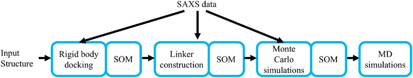
FIGURE 1. The workflow of the method. The main steps of the algorithm are depicted: rigid body docking, linker construction, Monte Carlo simulations, and Molecular Dynamics (MD) simulations. The Small-angle X-ray scattering (SAXS) data is used to derive the first three steps.
2.2.1 Rigid Body Docking
We started with 64 parallel simulations by placing the PDZ domain randomly around the PTP domain (without the linker and termini), avoiding physical contact between the two proteins (Figures 2A,B). The simulations rapidly converged to two distinct sets of conformations in which the PDZ domain (Figure 2C) is located on either of the two most distant points of the phosphatase domain, each subdivided in two further conformations (Figures 2D,E). In these conformations, the α2-helix of the PDZ domain is roughly aligned with the main axis of the phosphatase domain. This indicates a preferred orientation of the PDZ domain relative to the PTP domain.
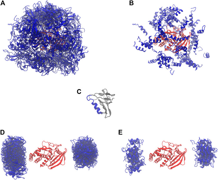
FIGURE 2. Starting and final conformations of the 64 rigid body simulations. PDZ in blue, PTP in red. (A) Starting conformations (full PDZ). (B) Starting conformations (only
To analyse the trajectories, we trained a self-organizing map (SOM) Bouvier et al. (2015). The subdivision of the two distinct sets of conformations into two further sets is clearly visible in the SOM, making it possible to define a total of four clusters (Figure 3A). Each cluster corresponds to one of the four possible combinations of position of the PDZ domain, and orientation of the α2-helix of the PDZ domain, with respect to the main axis of the phosphatase domain.
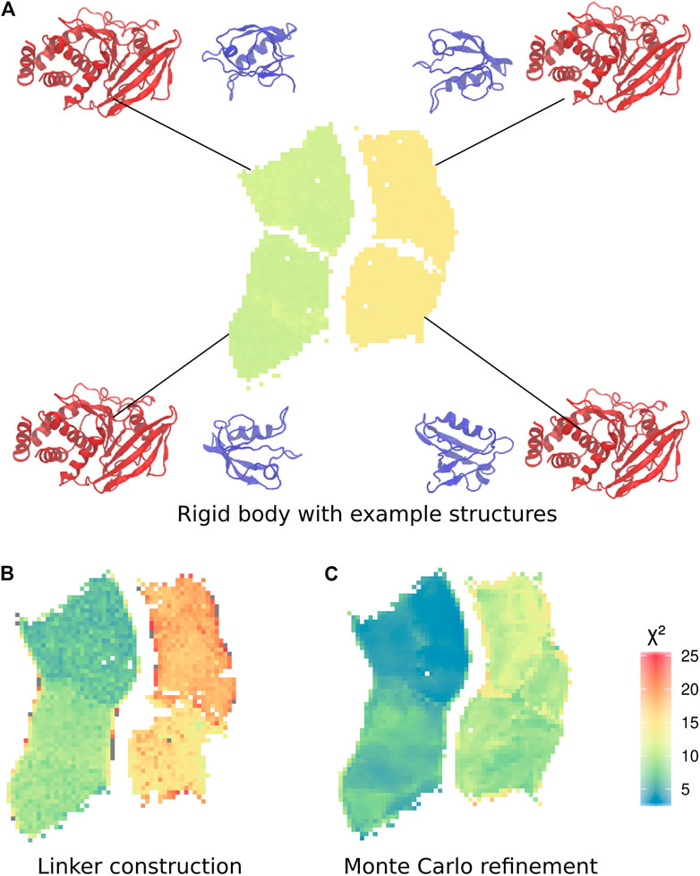
FIGURE 3. Self-organizing maps (SOMs) of the three calculation stages. (A) Final conformations of the rigid body docking stage, coloured by
2.2.2 Linker Construction
We then extracted a clash-free conformation displaying the lowest
2.2.3 Monte-Carlo Refinement
To further improve the sampling of the conformational space of the linker and termini, we performed an exhaustive refinement of the best structures of each neuron of the SOM map. We used a Monte-Carlo algorithm to sample the linker conformations in the dihedral angles of the linker and termini. As previously, we used only the Bayesian SAXS scoring term and volume exclusion to calculate the energy. This approach allowed the added residues and the domains to adjust jointly to the SAXS profile. The
The 10 conformations with the best final
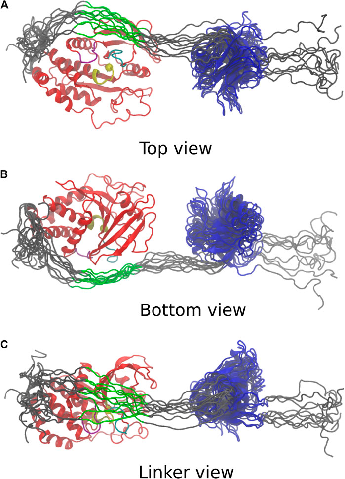
FIGURE 4. Last frame of the top 10 simulations, aligned on the PTP domain. PTP: red; PTP loop and catalytic cytosine [H (851)CSAGIGRT (859)]: yellow; WPD loop [W (818)PDHGVP(824)]: purple; β5-loop-β6 region [T (754)QVERGRV (761)]: cyan; C-terminus, N-terminus and linker: grey; highly conserved linker region [E (617)PDFQYIP(624)]: green; PDZ: blue. (A) Top view depicts catalytic site in vicinity to the linker. (B) Bottom view adopts same orientation as Figure 3. (C) Linker view shows conformational variability of linker.
2.2.4 Influence of the Weight Adjustment
During the calculations, the weight of the Bayesian SAXS score adjusted substantially (Figure 5). From the initial rigid body docking to the best structure after refinement, the weight was multiplied by 17. This means that the SAXS data was given 17 times more importance at the end of the procedure compared to the beginning. To see why this matters, we performed 20 linker refinement simulations with a fixed weight for the SAXS restraint, varying from 10−4–102 and compared it to 10 simulations using the Bayesian SAXS restraint. We then examined the
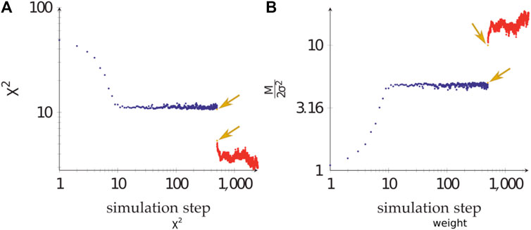
FIGURE 5. The adjustment of the Bayesian SAXS score. (A)
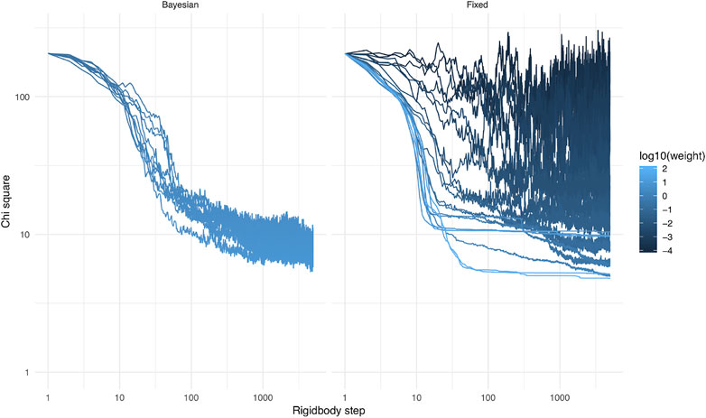
FIGURE 6.
2.3 Stability of the Optimal Conformation
2.3.1 Molecular Dynamics Simulations and Conformational Clustering
To further assess the stability of the optimal conformation obtained from the Bayesian analysis, we performed three MD simulations of 200 ns starting from the model with lowest
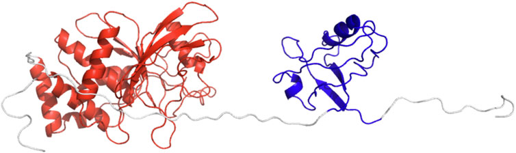
FIGURE 7. The cartoon representation of starting conformation for the MD simulations. PDZ is colored in blue and PTP in red.
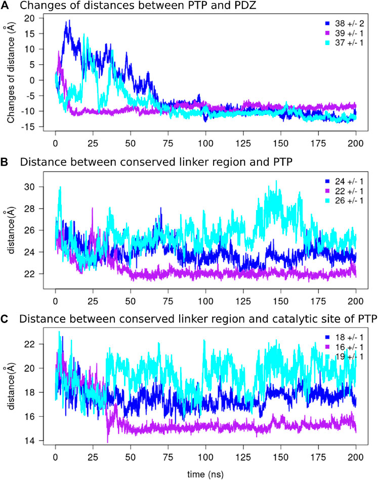
FIGURE 8. The distances along the MD simulations.(A) The changes of distances between the two domains and the average values over the final 125 ns of the simulations are reported for each replicate. The distance between the center of mass of the conserved linker region [E (617)PDFQYIP(624)] and the center of mass of (B) the PTP domain and (C) the catalytic site of the PTP domain are depicted for each replicate.
To better characterize the observed conformational transitions along the MD simulations of PTPN4, we clustered the set of conformations with the Self Organizing Maps (SOM) method already used above Bouvier et al. (2015). A total of 60 clusters were retrieved from a pool of 60,000 conformations (Figure 9). We then projected the
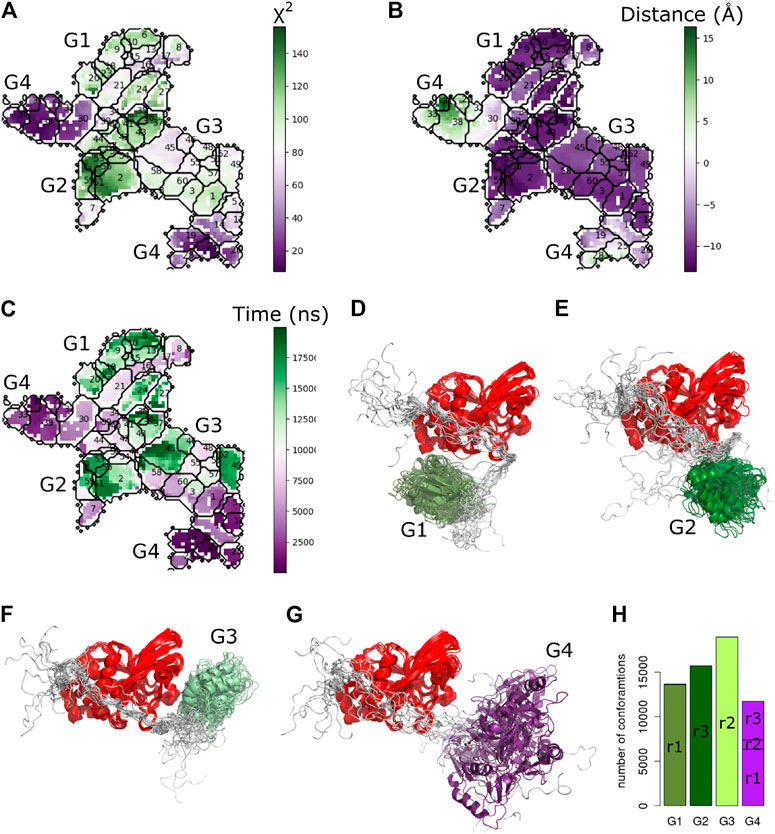
FIGURE 9. Cluster analysis of PTPN4 from the MD simulations. The self-organizing map of the PTPN4 conformations colored by (A)
To investigate overall convergence of the simulations, we analyzed the number of conformations from different replicates in each group (Figure 9H). The three replicates cover rather different conformational space. The groups G1, G2, and G3 contain conformations from only one replicate. Interestingly, only G4, which is the closest one to the starting conformation and has the lowest
2.3.2 Selection of Minimal Small Angle X-ray Scattering Ensemble
The above analysis assumes that a single structure or an ensemble covering a small part of conformational space represents the SAXS data. The sampling of conformational space by the free MD trajectories enabled us to try to investigate if more disperse ensembles fit the SAXS data better. For this, we used a method based on the genetic algorithm (GA) that was developed for a similar problem Delhommel et al. (2017). This method searches for the minimal subset of conformations minimizing the error between the experimental data and computed data from the MD simulations. The
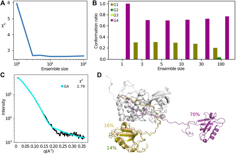
FIGURE 10. Extracting a minimum subset of conformations from the MD simulations, that describes best the SAXS data using a genetic algorithm. (A) Improvement of the
3 Discussion
3.1 Automatic Weight Adjustment
In general, and also in the Bayesian formalism, the SAXS scoring term is based on
3.2 Influence of the Weight Adjustment
As an illustration, suppose structure determination is performed with a bad guess for the initial structure. In this case,
Note that, the σ is being adjusted on the fly, and the maximum likelihood estimate of σ is approximately
3.3 Fixed Weight vs. Bayesian Automatic Weighting
The optimal weight, at which the simulation has reasonable acceptance rates and makes good use of SAXS information, is a priori unknown. It is the purpose of the Bayesian SAXS restraint to determine this optimal weight. As shown in Supplementary Equation S4 (see Supplementary Material), the number of SAXS data points and the overall agreement of data and structures will greatly influence the optimal weight. Therefore, it is expected that it will be different for each SAXS dataset, but also for each simulation setting, for example depending on which force field is used.
3.4 Log Score vs. Linear Score
An equivalent form for the Bayesian score without any additional parameter σ can be derived by an operation called marginalization (Supplementary Equation S5, Supplementary Material). As shown for NMR data Habeck et al. (2006), this form is equivalent to the weighted
3.5 A Point on Exhaustivity
The calculations presented here attempted to sample a large part of the conformational space of this two-domain system, since the energy landscape can be expected to be rugged. We showed that the energy surface is less rugged when using automatically adapted weights. The strength of this Bayesian restraint is that, regardless of the initial conformation, the calculations converge to low
3.6 Protein Tyrosine Phosphatase Non-Receptor 4
Using the novel Bayesian SAXS restraint, we have shown a conserved sequence in the linker of PTPN4, involved in the allosteric regulation of PTPN4 Caillet-Saguy et al. (2017), is facing both the β5-loop-β6 region and the WPD loop. The β5-loop-β6 region is thought to participate in defining substrate specificity Andersen et al. (2001). The WPD loop is well-known to be important for the phosphatase catalysis. The WPD loop switches from an open to close position upon substrate binding and adopts a catalytically active close conformation Barr et al. (2009). Previous experimental evidence showed that the linker participates in the control of the catalytic activity of the phosphatase domain Maisonneuve et al. (2014).
Mutations of a conserved hydrophobic patch in the linker suggested that the linker modulates the WPD loop open/closed conformations Caillet-Saguy et al. (2017). The close proximity of the linker with the β5-loop-β6 region and the WPD loop observed in our simulations further supports and reinforces the current model in which the linker of PTPN4 could regulate the phosphatase activity of PTPN4 by modulating the WPD loop closure.
3.7 Ensemble Modelling
The focus of this study is to illustrate the power and utility of the Bayesian SAXS score. The setup was deliberately simple, to emphasize to what degree the final conformations were driven by the data. Emphasis was also on calculation efficiency, and the molecule was deliberately described in the simplest terms by excluding volume, rigid bodies for the two domains, and rigid covalent geometry. The experimental data was limited to SAXS data up to
The conformations we obtain can serve as the basis of more detailed simulations with state of the art ensemble methods Potrzebowski et al. (2018), Shrestha et al. (2019), Paissoni et al. (2020). For a system of rather moderate size as the PTPN4 tandem (52 kDa), one could obviously directly refine against the data in a complete force field Shevchuk and Hub (2017). This would not allow for as extensive searching of conformational space as it was performed in this work. The aim of the current calculation protocol is to sample large relevant parts of conformational space efficiently, a task that is difficult to perform for large fully solvated molecules. An adaptation of the Bayesian SAXS restraint with automated weighting as described here could be useful also in this context. We note that such adaptation however, would not address the issue of multiple conformations representing the SAXS data. In this study we proposed a method to overcome this problem by first concentrating on obtaining the dominate conformational ensemble in a largely simplified force field without explicit solvent, and then further exploring a larger ensemble by a free, fully solvated simulation, and finally obtaining an optimal, small ensemble by combining different conformations from these simulations. While the best conformer obtained by Bayesian SAXS restraint has
4 Materials and Methods
4.1 Protein Production and Data Collection
The PDZ-PTPC/S construct, harboring the mutant C852S, hereafter referred to as PTPN4, was expressed and purified as previously described Maisonneuve et al. (2014). SAXS experiments were carried out as previously described except that the protein concentration used for SAXS experiments was 75 μM Maisonneuve et al. (2014).
4.2 Rigid Body Docking
In the first stage, we used IMP Russel et al. (2012) to perform rigid body docking of the PDB structures of PTP (PDB code 2I75; residues 638–913) and PDZ (PDB code 3NFK chain B; residues 512–604). 64 different simulations were performed with 500 steps each. Initial orientations of PDZ with respect to PTP cover a wide range of orientations both around the PTP and of the PDZ itself (see Figure 2). Energy terms were the SAXS restraint (Supplementary Equation S7) and a quadratic volume exclusion term. The FoXS model was used on heavy atoms Schneidman-Duhovny et al. (2013). Each step consisted in alternating 100 Monte Carlo rotation/translation moves
4.3 Rigid Body Self Organizing Map
A 50 × 50 SOM Bouvier et al. (2015), Spill et al. (2013) was trained on the last 200 frames of each of the 64 simulations. Specifically, we used descriptors with seven dimensions, extracted from the structures as follows. The coordinates of all 12,800 structures were recalculated in a reference frame in which the center of mass of PTP is at the origin, and its orientation is constant across the structures. The first three dimensions of the descriptors are the center of mass of PDZ in this reference frame, while the last four are the quaternions of the rotation of PDZ with respect to PTP. The metric used to compare a neuron n and a descriptor m is a weighted sum between euclidean distance between the center of masses and geodesic distance between the quaternions Huynh (2009).
where
4.4 Linker Modeling
In the second stage, we added linkers to our models. Due to the particular choice of the format of the SOM descriptors, a 3D structure can be reconstructed from the coordinates of the trained neurons. 1,999 clash-free structures could be extracted from the SOM neurons in such a way.
Missing residues were added with IMP Russel et al. (2012) so that the modeled part of the protein spanned residues 496–926. The termini were assigned random
The linker was generated in two steps. First,
Second, all atoms were placed around their corresponding
On average, this step resulted in 1,224 structures per pose, or a total of 2,461,844 structures.
4.5 Monte Carlo Refinement
For each of the 1,999 rigid body poses, the structure with linkers which had the best Bayesian SAXS score was used as starting conformation for a Monte Carlo refinement simulation. Each simulation consisted of 2,000 steps, each of which was an alternation between 10 Monte Carlo moves and optimization of σ and γ. Each Monte Carlo move was made in internal coordinates, and consisted in a Gaussian perturbation of the backbone dihedrals of residues 496–511, 606–636, and 914–926. The standard deviation of the Gaussian was
4.6 Fixed-Weight Small-angle X-ray scattering Simulations
To compare fixed-weight and self-adjusting simulations, we used a similar setup. 20 fixed-weight simulations were performed with a SAXS restraint with a weight spaced logarithmically from
4.7 Molecular Dynamics Simulations
We selected the top PTPN4 conformation determined using the Bayesian SAXS score, i.e., the one with the lowest
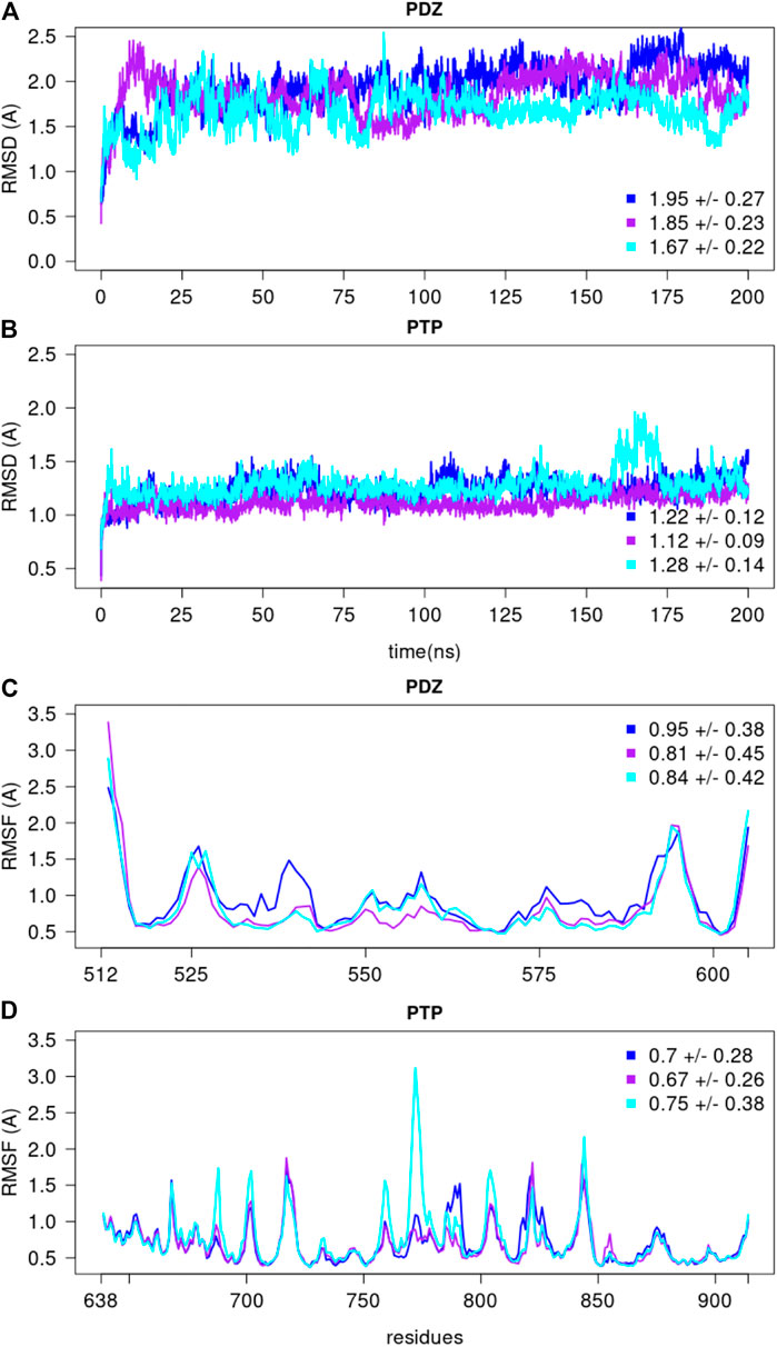
FIGURE 11. The root mean square deviations and fluctuations of each MD simulation. The RMSD over backbone atoms (Cα, C, N, O) measured from the initial structure are shown for the (A) PDZ and (B) PTP domains. The residue RMSF over backbone atoms (Cα, C, N, O) measured with respect to the average conformation are depicted for the (C) PDZ and (D) PTP domains, over the last 150 ns of each replicate. The average and standard deviation values are reported for every replicate.
4.8 Back Calculated Small-angle X-ray scattering Profiles
For every conformation of the MD simulations, the theoretical scattering profiles were calculated using CRYSOL from the ATSAS 2.8.3 software suite Svergun et al. (1995), with the default parameters. Their corresponding
where M is the number of points in SAXS profile,
4.9 Genetic Algorithm
We followed a similar procedure as in Delhommel et al. (2017), in which 1,000 steps of GA were performed, the number of generated ensemble was set to 1,000 with a cross over frequency of 0.8 and a mutation frequency of one. We performed the GA for different ensemble sizes: 1, 3, 5, 30, and 100. In addition, the GA was repeated five times for every ensemble size and average values were reported.
Data Availability Statement
The datasets presented in this study can be found in online repositories. The names of the repository/repositories and accession number(s) can be found below: The SAXS data, refined structures, and MD simulation trajectories generated for the PTPN4 for this study are deposited in the Zenodo. org database (accession doi: 10.5281/zenodo.4739101). Direct link: https://zenodo.org/record/4739101.
Author Contributions
All authors wrote and reviewed the article.
Funding
This work was supported by The Fondation pour la Recherche Medicale (Equipe FRM 2017M.DEQ20170839114) to YK and MN. PM was supported by grants from the Ministère de l'Enseignement Supérieur et de la Recherche and the Fondation pour la Recherche Médicale (FDT20130927999).
Conflict of Interest
The authors declare that the research was conducted in the absence of any commercial or financial relationships that could be construed as a potential conflict of interest.
Acknowledgments
The SAXS data, refined structure, and MD simulation trajectories generated for the PTPN4 for this study are deposited in the Zenodo.org database (accession doi: 10.5281/zenodo.4739101).
Supplementary Material
The Supplementary Material for this article can be found online at: https://www.frontiersin.org/articles/10.3389/fmolb.2021.671011/full#supplementary-material
References
Andersen, J. N., Mortensen, O. H., Peters, G. H., Drake, P. G., Iversen, L. F., Olsen, O. H., et al. (2001). Structural and Evolutionary Relationships Among Protein Tyrosine Phosphatase Domains. Mol. Cel. Biol. 21, 7117–7136. doi:10.1128/mcb.21.21.7117-7136.2001
Babault, N., Cordier, F., Lafage, M., Cockburn, J., Haouz, A., Prehaud, C., et al. (2011). Peptides Targeting the PDZ Domain of PTPN4 Are Efficient Inducers of Glioblastoma Cell Death. Structure 19, 1518–1524. doi:10.1016/j.str.2011.07.007
Barr, A. J., Ugochukwu, E., Lee, W. H., King, O. N. F., Filippakopoulos, P., Alfano, I., et al. (2009). Large-scale Structural Analysis of the Classical Human Protein Tyrosine Phosphatome. Cell 136, 352–363. doi:10.1016/j.cell.2008.11.038
Berendsen, H. J. C., Postma, J. P. M., van Gunsteren, W. F., DiNola, A., and Haak, J. R. (1984). Molecular Dynamics with Coupling to an External bath. J. Chem. Phys. 81, 3684–3690. doi:10.1063/1.448118
Bernard, A., Vranken, W. F., Bardiaux, B., Nilges, M., and Malliavin, T. E. (2011). Bayesian Estimation of NMR Restraint Potential and Weight: a Validation on a Representative Set of Protein Structures. Proteins 79, 1525–1537. doi:10.1002/prot.22980
Bonomi, M., Hanot, S., Greenberg, C. H., Sali, A., Nilges, M., Vendruscolo, M., et al. (2019). Bayesian Weighing of Electron Cryo-Microscopy Data for Integrative Structural Modeling. Structure 27, 175–188. doi:10.1016/j.str.2018.09.011
Bouvier, G., Desdouits, N., Ferber, M., Blondel, A., and Nilges, M. (2015). An Automatic Tool to Analyze and Cluster Macromolecular Conformations Based on Self-Organizing Maps. Bioinformatics 31, 1490–1492. doi:10.1093/bioinformatics/btu849
Brünger, A. T. (1992). Free R Value: a Novel Statistical Quantity for Assessing the Accuracy of crystal Structures. Nature 355, 472–475. doi:10.1038/355472a0
Caillet-Saguy, C., Maisonneuve, P., Delhommel, F., Terrien, E., Babault, N., Lafon, M., et al. (2015). Strategies to Interfere with PDZ-Mediated Interactions in Neurons: What We Can Learn from the Rabies Virus. Prog. Biophys. Mol. Biol. 119, 53–59. doi:10.1016/j.pbiomolbio.2015.02.007
Caillet-Saguy, C., Toto, A., Guerois, R., Maisonneuve, P., Di Silvio, E., Sawyer, K., et al. (2017). Regulation of the Human Phosphatase PTPN4 by the Interdomain Linker Connecting the PDZ and the Phosphatase Domains. Scientific Rep. 7, 2–10. doi:10.1038/s41598-017-08193-6
Chen, P.-c., and Hub, J. S. (2015). Interpretation of Solution X-ray Scattering by Explicit-Solvent Molecular Dynamics. Biophysical J. 108, 2573–2584. doi:10.1016/j.bpj.2015.03.062
Darden, T., York, D., and Pedersen, L. (1993). Particle Mesh Ewald: AnN⋅Log(N) Method for Ewald Sums in Large Systems. J. Chem. Phys. 98, 10089–10092. doi:10.1063/1.464397
Delhommel, F., Cordier, F., Bardiaux, B., Bouvier, G., Colcombet-Cazenave, B., Brier, S., et al. (2017). Structural Characterization of Whirlin Reveals an Unexpected and Dynamic Supramodule Conformation of its PDZ Tandem. Structure 25, 1645–1656. doi:10.1016/j.str.2017.08.013
Dill, K. A., and Chan, H. S. (1997). From Levinthal to Pathways to Funnels: The ”New View” of Protein Folding Kinetics. Nat. Struct. Biol. 4, 10.
Ferber, M., Kosinski, J., Ori, A., Rashid, U. J., Moreno-Morcillo, M., Simon, B., et al. (2016). Automated Structure Modeling of Large Protein Assemblies Using Crosslinks as Distance Restraints. Nat. Methods 13, 515–520. doi:10.1038/nmeth.3838
Gu, M., and Majerus, P. W. (1996). The Properties of the Protein Tyrosine Phosphatase PTPMEG. J. Biol. Chem. 271, 27751–27759. doi:10.1074/jbc.271.44.27751
Gu, M., Meng, K., and Majerus, P. W. (1996). The Effect of Overexpression of the Protein Tyrosine Phosphatase PTPMEG on Cell Growth and on colony Formation in Soft agar in COS-7 Cells. Proc. Natl. Acad. Sci. 93, 12980–12985. doi:10.1073/pnas.93.23.12980
Habeck, M., Rieping, W., and Nilges, M. (2006). Weighting of Experimental Evidence in Macromolecular Structure Determination. Proc. Natl. Acad. Sci. 103, 1756–1761. doi:10.1073/pnas.0506412103
Huang, J., Rauscher, S., Nawrocki, G., Ran, T., Feig, M., de Groot, B. L., et al. (2017). CHARMM36m: an Improved Force Field for Folded and Intrinsically Disordered Proteins. Nat. Methods 14, 71–73. doi:10.1038/nmeth.4067
Huynh, D. Q. (2009). Metrics for 3d Rotations: Comparison and Analysis. J. Math. Imaging Vis. 35, 155–164. doi:10.1007/s10851-009-0161-2
Jorgensen, W. L., Chandrasekhar, J., Madura, J. D., Impey, R. W., and Klein, M. L. (1983). Comparison of Simple Potential Functions for Simulating Liquid Water. J. Chem. Phys. 79, 926–935. doi:10.1063/1.445869
Kina, S.-i., Tezuka, T., Kusakawa, S., Kishimoto, Y., Kakizawa, S., Hashimoto, K., et al. (2007). Involvement of Protein-Tyrosine Phosphatase PTPMEG in Motor Learning and Cerebellar Long-Term Depression. Eur. J. Neurosci. 26, 2269–2278. doi:10.1111/j.1460-9568.2007.05829.x
Kohda, K., Kakegawa, W., Matsuda, S., Yamamoto, T., Hirano, H., and Yuzaki, M. (2013). The 2 Glutamate Receptor gates Long-Term Depression by Coordinating Interactions between Two AMPA Receptor Phosphorylation Sites. Proc. Natl. Acad. Sci. 110, E948–E957. doi:10.1073/pnas.1218380110
Loncharich, R. J., Brooks, B. R., and Pastor, R. W. (1992). Langevin Dynamics of Peptides: The Frictional Dependence of Isomerization Rates ofN-Acetylalanyl-N?-Methylamide. Biopolymers 32, 523–535. doi:10.1002/bip.360320508
MacKerell, A. D., Bashford, D., Bellott, M., Dunbrack, R. L., Evanseck, J. D., Field, M. J., et al. (1998). All-Atom Empirical Potential for Molecular Modeling and Dynamics Studies of Proteins†. J. Phys. Chem. B 102, 3586–3616. doi:10.1021/jp973084f
Maisonneuve, P., Caillet-Saguy, C., Raynal, B., Gilquin, B., Chaffotte, A., Pérez, J., et al. (2014). Regulation of the Catalytic Activity of the Human Phosphatase Ptpn4 by its Pdz Domain. Febs J. 281, 4852–4865. doi:10.1111/febs.13024
Maisonneuve, P., Caillet-Saguy, C., Vaney, M.-C., Bibi-Zainab, E., Sawyer, K., Raynal, B., et al. (2016). Molecular Basis of the Interaction of the Human Protein Tyrosine Phosphatase Non-receptor Type 4 (PTPN4) with the Mitogen-Activated Protein Kinase P38γ. J. Biol. Chem. 291, 16699–16708. doi:10.1074/jbc.m115.707208
Mareuil, F., Sizun, C., Perez, J., Schoenauer, M., Lallemand, J.-Y., and Bontems, F. (2007). A Simple Genetic Algorithm for the Optimization of Multidomain Protein Homology Models Driven by NMR Residual Dipolar Coupling and Small Angle X-ray Scattering Data. Eur. Biophys. J. 37, 95–104. doi:10.1007/s00249-007-0170-2
Nilges, M., Bernard, A., Bardiaux, B., Malliavin, T., Habeck, M., and Rieping, W. (2008). Accurate NMR Structures through Minimization of an Extended Hybrid Energy. Structure 16, 1305–1312. doi:10.1016/j.str.2008.07.008
Paissoni, C., Jussupow, A., and Camilloni, C. (2020). Determination of Protein Structural Ensembles by Hybrid-Resolution SAXS Restrained Molecular Dynamics. J. Chem. Theor. Comput. 16, 2825–2834. doi:10.1021/acs.jctc.9b01181
Phillips, J. C., Braun, R., Wang, W., Gumbart, J., Tajkhorshid, E., Villa, E., et al. (2005). Scalable Molecular Dynamics with NAMD. J. Comput. Chem. 26, 1781–1802. doi:10.1002/jcc.20289
Potrzebowski, W., Trewhella, J., and Andre, I. (2018). Bayesian Inference of Protein Conformational Ensembles from Limited Structural Data. Plos Comput. Biol. 14, e1006641. doi:10.1371/journal.pcbi.1006641
Préhaud, C., Wolff, N., Terrien, E., Lafage, M., Mégret, F., Babault, N., et al. (2010). Attenuation of Rabies Virulence: Takeover by the Cytoplasmic Domain of its Envelope Protein. Sci. Signaling 3, ra5. doi:10.1126/scisignal.2000510
Rieping, W., Habeck, M., and Nilges, M. (2005). Inferential Structure Determination. Science 309, 303–306. doi:10.1126/science.1110428
Rozycki, B., Kim, Y. C., and Hummer, G. (2011). SAXS Ensemble Refinement of ESCRT-III CHMP3 Conformational Transitions. Structure 19, 109–116.
Russel, D., Lasker, K., Webb, B., Velázquez-Muriel, J., Tjioe, E., Schneidman-Duhovny, D., et al. (2012). Putting the Pieces Together: Integrative Modeling Platform Software for Structure Determination of Macromolecular Assemblies. Plos Biol. 10, e1001244. doi:10.1371/journal.pbio.1001244
Schneidman-Duhovny, D., Hammel, M., Tainer, J. A., and Sali, A. (2013). Accurate SAXS Profile Computation and its Assessment by Contrast Variation Experiments. Biophysical J. 105, 962–974. doi:10.1016/j.bpj.2013.07.020
Shevchuk, R., and Hub, J. S. (2017). Bayesian Refinement of Protein Structures and Ensembles against SAXS Data Using Molecular Dynamics. Plos Comput. Biol. 13, e1005800. doi:10.1371/journal.pcbi.1005800
Shrestha, U. R., Juneja, P., Zhang, Q., Gurumoorthy, V., Borreguero, J. M., Urban, V., et al. (2019). Generation of the Configurational Ensemble of an Intrinsically Disordered Protein from Unbiased Molecular Dynamics Simulation. Proc. Natl. Acad. Sci. USA 116, 20446–20452. doi:10.1073/pnas.1907251116
Spill, Y. (2013). Développement de méthodes d’échantillonnage et traitement bayésien de données continues: nouvelle méthode d’échange de répliques et modélisation de données SAXS. Ph.D. Thesis, Paris 7.
Spill, Y. G., Bouvier, G., and Nilges, M. (2013). A Convective Replica-Exchange Method for Sampling New Energy Basins. J. Comput. Chem. 34, 132–140. doi:10.1002/jcc.23113
Spill, Y. G., Kim, S. J., Schneidman-Duhovny, D., Russel, D., Webb, B., Sali, A., et al. (2014). Saxs Merge: an Automated Statistical Method to Merge Saxs Profiles Using Gaussian Processes. J. Synchrotron Radiat. 21, 203–208. doi:10.1107/s1600577513030117
Svergun, D., Barberato, C., and Koch, M. H. J. (1995). CRYSOL- a Program to Evaluate X-ray Solution Scattering of Biological Macromolecules from Atomic Coordinates. J. Appl. Cryst. 28, 768–773. doi:10.1107/s0021889895007047
Yang, S., Blachowicz, L., Makowski, L., and Roux, B. (2010). Multidomain Assembled States of Hck Tyrosine Kinase in Solution. Proc. Natl. Acad. Sci. 107, 15757–15762. doi:10.1073/pnas.1004569107
Young, J. A., Becker, A. M., Medeiros, J. J., Shapiro, V. S., Wang, A., Farrar, J. D., et al. (2008). The Protein Tyrosine Phosphatase PTPN4/PTP-MEG1, an Enzyme Capable of Dephosphorylating the TCR ITAMs and Regulating NF-Κb, Is Dispensable for T Cell Development And/or T Cell Effector Functions. Mol. Immunol. 45, 3756–3766. doi:10.1016/j.molimm.2008.05.023
Zhang, B. D., Li, Y. R., Ding, L. D., Wang, Y. Y., Liu, H. Y., and Jia, B. Q. (2019). Loss of PTPN4 Activates STAT3 to Promote the Tumor Growth in Rectal Cancer. Cancer Sci. 110, 2258–2272. doi:10.1111/cas.14031
Keywords: SAXS, bayesian scoring, automatic weighting, inferential structure determination, PTPN4, allosteric regulation, conformational dynamics
Citation: Spill YG, Karami Y, Maisonneuve P, Wolff N and Nilges M (2021) Automatic Bayesian Weighting for SAXS Data. Front. Mol. Biosci. 8:671011. doi: 10.3389/fmolb.2021.671011
Received: 22 February 2021; Accepted: 14 May 2021;
Published: 04 June 2021.
Edited by:
Gregory Bowman, Washington University School of Medicine in St. Louis, United StatesReviewed by:
Kresten Lindorff-Larsen, University of Copenhagen, DenmarkJochen Hub, Saarland University, Germany
Copyright © 2021 Spill, Karami, Maisonneuve, Wolff and Nilges. This is an open-access article distributed under the terms of the Creative Commons Attribution License (CC BY). The use, distribution or reproduction in other forums is permitted, provided the original author(s) and the copyright owner(s) are credited and that the original publication in this journal is cited, in accordance with accepted academic practice. No use, distribution or reproduction is permitted which does not comply with these terms.
*Correspondence: Michael Nilges, michael.nilges@pasteur.fr
†These authors have contributed equally to this work and share first authorship.