Single channel approach for filtering electroencephalographic signals strongly contaminated with facial electromyography
 Carlos Magno Medeiros Queiroz1
  Gustavo Moreira da Silva1
  Steffen Walter2*
  Luciano Brinck Peres1
  Luiza Maire David Luiz1
  Samila Carolina Costa1
  Kelly Christina de Faria1
  Adriano Alves Pereira1
  Marcus Fraga Vieira3
  Ariana Moura Cabral1
  Adriano de Oliveira Andrade1
- 1Centre for Innovation and Technology Assessment in Health, Federal University of Uberlândia, Uberlândia, Brazil
- 2Department of Medical Psychology, Clinic of Psychosomatic Medicine and Psychotherapy, University Hospital Ulm, Ulm, Germany
- 3Bioengineering and Biomechanics Laboratory, Federal University of Goiás, Goiânia, Brazil
Eliminating facial electromyographic (EMG) signal from the electroencephalogram (EEG) is crucial for the accuracy of applications such as brain computer interfaces (BCIs) and brain functionality measurement. Facial electromyography typically corrupts the electroencephalogram. Although it is possible to find in the literature a number of multi-channel approaches for filtering corrupted EEG, studies employing single-channel approaches are scarce. In this context, this study proposed a single-channel method for attenuating facial EMG noise from contaminated EEG. The architecture of the method allows for the evaluation and incorporation of multiple decomposition and adaptive filtering techniques. The decomposition method was responsible for generating EEG or EMG reference signals for the adaptive filtering stage. In this study, the decomposition techniques CiSSA, EMD, EEMD, EMD-PCA, SSA, and Wavelet were evaluated. The adaptive filtering methods RLS, Wiener, LMS, and NLMS were investigated. A time and frequency domain set of features were estimated from experimental signals to evaluate the performance of the single channel method. This set of characteristics permitted the characterization of the contamination of distinct facial muscles, namely Masseter, Frontalis, Zygomatic, Orbicularis Oris, and Orbicularis Oculi. Data were collected from ten healthy subjects executing an experimental protocol that introduced the necessary variability to evaluate the filtering performance. The largest level of contamination was produced by the Masseter muscle, as determined by statistical analysis of the set of features and visualization of topological maps. Regarding the decomposition method, the SSA method allowed for the generation of more suitable reference signals, whereas the RLS and NLMS methods were more suitable when the reference signal was derived from the EEG. In addition, the LMS and RLS methods were more appropriate when the reference signal was the EMG. This study has a number of practical implications, including the use of filtering techniques to reduce EEG contamination caused by the activation of facial muscles required by distinct types of studies. All the developed code, including examples, is available to facilitate a more accurate reproduction and improvement of the results of this study.
1. Introduction
Electroencephalography is a technique used to record the activity on the scalp of measured cerebral cortex neuronal populations. It is derived from a high temporal resolution, non-invasive macroscopic process and is a low-cost method compared to a functional neuroimaging test (Pivik et al., 1993; McMenamin et al., 2011; Mamun et al., 2013). The electroencephalogram (EEG) is widely used in a variety of clinical and commercial applications, including cognitive neuroscience, brain-skill quantification, pathological diagnosis, biometrics, and Brain-Computer Interfaces (BCIs) (Foxe and Snyder, 2011; Abo-Zahhad et al., 2015; Mihajlovic et al., 2015; Ramadan and Vasilakos, 2017).
The system for measuring EEG amplifies the tiny disturbances of the electrical potentials of the electrodes positioned on the scalp, which is anatomically separated from the signal-generating sources by the meninges, skull bones, and scalp. Thus, the synaptic potentials which usually have low amplitudes, in the order of millivolts, are strongly attenuated by these anatomical structures, reducing the amplitude of the signals recorded at the scalp (Hero, 2006). Due to this low amplitude, which typically does not exceed 100 μV, the EEG signal is highly susceptible to artifacts. These artifacts are usually caused by electromagnetic fields generated by nearby electronic devices and the power grid. In addition, artifacts can be produced by other sources of electrophysiological signals, e.g., muscular and heart activity or eye movement (Sweeney et al., 2012; Urigüen and Garcia-Zapirain, 2015). This contamination decreases the performance of applications such as BCI and diagnosis of pathological disfunctions, since the amplitude of the artifact will typically be several orders of magnitude greater than the EEG amplitude (Nunez and Srinivasan, 2006; Tatum et al., 2011).
In this context, the characterization and elimination of artifacts is relevant for the correct interpretation and use of EEG. Facial electromyographic (EMG) signals are a primary source of EEG contamination. The main challenge with respect to the elimination of noise generated by the EMG signal lies in the fact that EMG emerges from the anatomically positioned muscles along the skull. Even weak muscular contractions can be detected throughout the scalp due to the phenomenon of conductive volume. In addition, the EMG signal overlaps the spectrum of the EEG signal in virtually all frequency bands (Goncharova et al., 2003).
To solve this problem, several EEG filtering methods are described in the literature. However, these methods have some limitations, mainly related to the inability to completely remove noise from the corrupted signal without the introduction of undesired distortions, and the need for a priori noise information for signal filtering. These limitations, associated with several features estimated from the EEG signal to suit the diversity of applications, motivate the search for multiple gold standards for removing EEG artifacts (Safieddine et al., 2012; Gabsteiger et al., 2014; Urigüen and Garcia-Zapirain, 2015; Bono et al., 2016; Upadhyay et al., 2016; Frølich and Dowding, 2018; Mucarquer et al., 2020).
Frequency selector filters, such as a linear Butterworth filter, are one of the main techniques described in the literature for the removal of physiological artifacts from EEG. However, the use of such filter class is only effective when the frequency range of the signal and noise are not overlapped (Sweeney et al., 2012).
The literature suggests the use of single-channel techniques for muscular artifact removal from EEG instead of multichannel techniques, e.g., Independent Component Analysis (ICA) and Canonical Correlation Analysis (CCA). The following methods are commonly employed for this purpose: adaptive filtering (Correa et al., 2007; Diniz, 2008; Kher and Gandhi, 2016); Wiener filtering (Maki et al., 2015; Ferdous and Ali, 2017), Bayesian filtering (Morbidi et al., 2008), Blind Source Separation (BSS) (James and Hesse, 2004; Albera et al., 2012), wavelet transform (WT) (Ngoc et al., 2015; Turnip and Pardede, 2017), Empirical Mode Decomposition (EMD) (Gaur et al., 2015; Alam and Samanta, 2017), and the combination of these techniques, i.e., hybrid methods (Chen et al., 2014; Daly et al., 2015; Salsabili et al., 2015; Bono et al., 2016; Zeng et al., 2016).
An adaptive filter is required when fixed specifications are unknown. The literature describes that the most prevalent family of algorithms for removing EEG artifacts is based on the method of least squares (Correa et al., 2007; Kim and Kim, 2018). Adaptive filters vary in time because their parameters are continuously changing to meet a performance requirement (Gerardo et al., 2011).
Wiener filtering is appropriate in situations in which the signal and noise spectrum are overlapping, although it requires an estimated, measured, or reliable reference to operate. Sengupta and Kay (1995) showed that the performance of the multichannel Wiener filter (MWF) outperformed that of BSS for removal of EEG artifacts of various types, i.e., those that were annotated as unwanted by the user. In addition, Ferdous and Ali (2017) compared Wiener and Kalman filters, and again the Wiener filter was more effective for removing EEG artifacts. However, the Wiener filter was mainly applied to remove ocular artifacts, not including muscular artifacts with low SNR, i.e., lower than −10 dB.
Gao et al. (2010) employed an adaptive algorithm to remove ECG from EEG during sleep apnea records by means of Discrete Wavelet Transform (DWT). Iyer and Zouridakis (2007) compared DWT with an ICA filter for subsequent detection of single-trial evoked potential. Krishnaveni et al. (2006) compared the Joint Approximation Diagonalization of Eigen-matrices (JADE) algorithm (Rutledge and Bouveresse, 2013) with DWT for the removal of EOG from EEG.
Empirical Mode Decomposition (EMD) was successfully used for the removal of EEG artifacts in Safieddine et al. (2012) and Zhang et al. (2012) and also in conjunction with BSS methods (Zhang et al., 2012; Sweeney, 2013). A broad review of the application of EMD and its variations on EEG signal processing is given in Sweeney-Reed et al. (2018).
Recent efforts have been focused on the combination of these algorithms for removing artifacts from the EEG. Hybrid methods are, therefore, considered the state of the art in EEG filtering because they use the advantages of different methods in two or more stages and have presented the best results in their applications (Castellanos and Makarov, 2006; Sweeney et al., 2012; Sweeney, 2013; Urigüen and Garcia-Zapirain, 2015; Bono et al., 2016; Mannan et al., 2016; Zeng et al., 2016; Frølich and Dowding, 2018). The main combinations of algorithms in different filtering stages are: (i) adaptive filtering with BSS-ICA; (ii) EMD with BSS; (iii) wavelet with BSS; (iv) adaptive filtering with EMD (Mannan et al., 2016).
Currently, single-channel techniques have been shown to be the most effective approach for the removal of facial muscular artifacts from EEG, especially when a reference signal is known (Chen et al., 2016). However, the main limitation of this class of noise removal technique is that its performance is low for signal-to-noise ratios below −10 dB (Chen et al., 2016; Zeng et al., 2016; Mucarquer et al., 2020), which is typical in EEG contaminated by facial electromyography. To the best of our knowledge, there is lack of studies addressing the removal of facial muscular artifacts from EEG. This is important when there is a need to monitor brain activity during human computer interaction (Andrade et al., 2013).
To contribute to the research on facial EMG removal from EEG, this study presents an EEG filtering approach for facial EMG removal that is independent of an external reference noise and suited for low SNR signals. The strategy involves determining a single channel reference signal using a decomposition technique, which is subsequently utilized by an adaptive filter to attenuate facial EMG. The reported results consider the evaluation of various decomposition and adaptive filtering methods, as well as the evaluation of filtering performance in the time and frequency domains. The experimental protocol used in this study is based on the practical need to assess brain activity for motor learning quantification during interaction with a myoelectric interface (Andrade et al., 2013).
2. Materials and methods
2.1. Experimental protocol
Data were collected from ten healthy individuals during the execution of successive facial muscular contractions to characterize the EEG signal contamination by facial muscular activity. This experimental protocol was based on previous published work (Andrade et al., 2013) reporting the implementation of a facial EMG interface and motor learning assessment.
This study followed the Resolution 466/2012 of the National Health Council. The study was conducted at the Centre for Innovation and Technology Assessment in Health of the Federal University of Uberlândia (UFU), Brazil. The experimental protocol was approved by the Human Research Ethics Committee (CEP-UFU), CAAE Number: 43670815.4.0000.5152.
The protocol consisted of two sets of facial muscle contractions, one with the eyes open and one with the eyes closed. The open and closed eyes conditions allowed for the evaluation of the filtering methods considering changes in the EEG amplitude. The participants were instructed to perform a series of facial expressions (Figure 1) by contracting five distinct muscles (Frontalis, Masseter, Orbicularis Oculi, Orbicularis Oris, and Zygomatic).

Figure 1. Participants were instructed to make a variety of facial expressions by activating muscles whose electrical activity corrupts the electroencephalogram. The facial expressions were performed with both open and closed eyes. In the neutral condition (A) there was no muscular contraction, whereas in the other conditions the following muscles were activated: Frontalis (B), Masseter (C), Orbicularis Oculi (D), Zygomatic (E), and Orbicularis Oris (F).
Each muscle was contracted 15 times following a random timing protocol (Figure 2) of three distinct patterns: long (3 s), medium (1 s), and short (0.5 s). The onset and duration of the contractions were controlled by an auditory stimulus (beep). The volunteer was asked to maintain the contraction while listening to the beep, and to finish the contraction immediately after the auditory stimulus considering these timing patterns. There were five repetitions of each contraction pattern. Each contraction was followed by a 2 s neutral period. Each participant performed 150 muscle contractions.
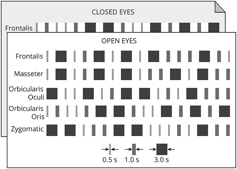
Figure 2. Each muscle was contracted 15 times in one of three timing patterns: long (3 s), medium (1 s), and short (0.5 s). Each pattern of contraction was repeated five times randomly. A 2-s neutral period followed each contraction. This protocol was executed with open and closed eyes.
Thus, for 10 participants, the data set consisted of 500 contractions lasting 3 s, 500 contractions lasting 1 s, and 500 contractions lasting 0.5 s, for a total of 2,250 s of EEG signals corrupted by facial EMG.
In this study the bipolar, i.e., differential, EEG montage was used to deliberately differentiating potentials between spatially adjacent locations as this may lead to improved signal-to-noise ratio of the collected signal. This type of configuration is also known as longitudinal configuration and widely employed in clinical practice (Kutluay and Kalamangalam, 2019). Although the employed montage was bipolar, the electrodes were positioned by using an EEG cap following the 10-20 International system of EEG electrode placement.
EMG signals were detected by using disposable sensors (Meditrace, USA) and collected simultaneously to EEG by using the RHD USB interface board (lntan, USA). The signals were sampled at 5 kHz and band-pass filtered (0.1 Hz–1 kHz).
2.2. Signal processing stages for the implementation of a single channel approach to EEG filtering
Figure 3 depicts the sequence of steps required to implement a single approach for filtering EEG signals corrupted by facial EMG. The first step is to eliminate any linear and non-linear trends from the collected signals. These tendencies are typically due in part to drift caused by changes in the impedance between the skin and the electrode, as well as cable and skin motion. By fitting a linear model to the time series and then subtracting the resulting straight line from the data, the linear trend is eliminated.
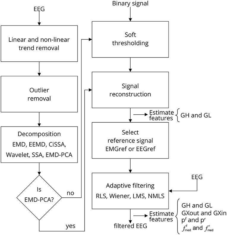
Figure 3. Filtering EEG signals corrupted by EMG via a series of steps. Linear and non-linear trends are eliminated, as well as outliers. The signal is then decomposed using one of the methods outlined, and the resulting components are thresholded. The thresholding process requires the identification of noise periods in the signal, which are provided by a binary signal generated by an EMG burst detector (Figure 4). Once the components have been thresholded, the filtered signal is reconstructed, producing a reference signal, i.e., EEG or EMG reference signal, which can be used as a reference for one of the indicated adaptive filters. Various characteristics are estimated to evaluate the filtering process at distinct stages. Note that when the method EMD-PCA is used it is not necessary to execute the soft-thresholding stage.
The non-linear trend is estimated by applying a sliding, non-overlapping, rectangular window of 20 ms (100 samples) to the data and then estimating the median of each window. The resultant time-series is interpolated using a Piecewise Cubic Hermite Interpolating Polynomial (pchip) so that it can be re-sampled with the same number of samples as the input time-series. The resultant signal is the non-linear trend that should be subtracted from the signal (i.e., the electroencephalogram or electromyogram). Supplementary Figure 1, which is available as Supplementary Material, shows an example of the result of this signal processing stage applied to an acquired EMG signal.
Outliers can result from any sudden abnormal changes in data amplitude that exceed or fall below predetermined thresholds. In this study, the upper/lower threshold was established as the mean plus/minus ten times the standard deviation of the data in the EMG-contaminated regions. The outliers were replaced by random scalars drawn from the standard normal distribution.
The pre-processed signal is then decomposed by one of the following decomposition methods: Empirical Mode Decomposition (EMD) (Huang et al., 1998), Extended Empirical Mode Decomposition (EEMD) (Wu and Huang, 2009), Circulant Singular Spectrum Analysis (CiSSA) (Bógalo et al., 2021), Wavelet Decomposition (Turnip and Pardede, 2017), or Singular Spectrum Analysis (SSA) (Bógalo et al., 2021). For the methods EMD, EEMD, CiSSA, and Wavelet, the maximum number of components was set to 10. For EMD and EEMD, the pchip interpolation method was utilized. For the EEMD approach, there were five ensembles. For Wavelet Decomposition, the mother wavelet was coif5. For the method SSA, the window length was 100 and the proportion of explained variance was 80%.
The obtained components are then soft-thresholded to eliminate noise as explained in a previous work (Andrade et al., 2006). For each signal component C = {c1, c2, ⋯ , cM}, a threshold, tm|m = {1, ⋯ , M}, is estimated, and soft-thresholding is applied to individual components as shown in Equation (1),
where tcm is the de-noised (or thresholded) version of the mth signal component and the function (x)+ is defined as
The threshold tm is estimated by using the following strategy: a window of noise is selected from the original signal and then the boundaries of this window are used to extract regions of noise from the signal components. For noise information selection, a binary signal is used. Low-level periods in this binary signal correspond to noise, while high-level periods correspond to EMG regions. Figure 4 provides an overview of the required steps for automatic EMG burst detection (Andrade et al., 2006). Although the EMG signal is the input signal illustrated in Figure 4, EMG bursts can be detected directly from EEG that has been corrupted by EMG. Because EMG signals were collected simultaneously with EEG, we decided not to use the EMG-corrupted EEG in this study for EMG burst detection.
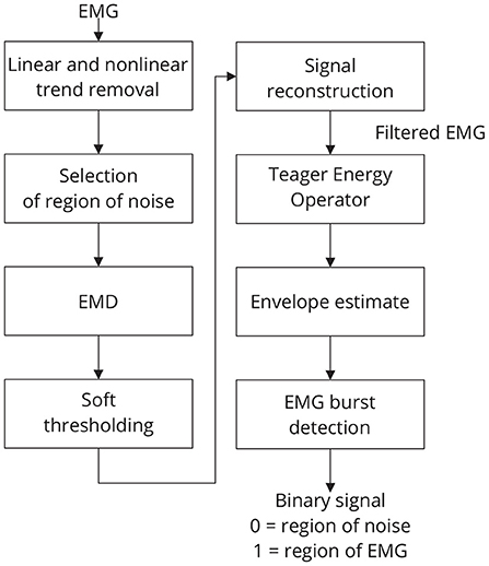
Figure 4. Sequence of required steps for detecting EMG bursts. First, the input signal is preprocessed by removing linear and nonlinear trends, and then the resulting signal is decomposed using EMD. The estimated components are soft-thresholded using a priori knowledge of the signal's noise level. Signal filtration is achieved by summing the thresholded components. The EMG envelope is determined by estimating the signal's energy, and bursts are detected using a threshold. As a result of this step, a binary signal is generated in which low levels indicate noise and high levels indicate EMG activity.
The standard deviation of each of those regions is then estimated, multiplied by a constant k, to obtain the required thresholds (t1, ..., tM). A typical value of k is 1.5 (Andrade et al., 2006). It is possible to vary k to control the signal filtering.
The EMG reference signal is obtained during the signal reconstruction stage. The adaptive filter may use this signal as a reference. Optionally, an EEG signal may be used as a reference. In this case, the noise-corrupted EEG is subtracted from the EMG reference signal to produce the EEG reference signal. Note that the reference signal is a filtered signal, resulting from the reconstruction of soft-thresholded signal components. In the case of the EMD-PCA method, the signal is reconstructed by selecting the principal components that account for at least 80% of the data variability. For the other methods, the signal is reconstructed based solely in the estimated components.
The reference signal is sent through an adaptive filter, which removes EMG noise from the electroencephalogram. One of the following adaptive filters can be chosen: Recursive Least Squares (RLS), Wiener filter, Least Mean Square (LMS), and Normalized Least Mean Square (NMLS) (Farhang-Boroujeny, 1999). Except for the method NMLS, which had an order of 4, the step-size utilized for all filters was 10−7 and the order was 10. Matlab R2022a was used to implement all of the code required for signal processing (MathWorks, USA).
2.3. Estimate of features for filtering assessment
Several features were estimated to enable for the characterization of EMG contamination on EEG and to compare different approaches used in the investigation. The stages in which the set of features is estimated are depicted in Figure 3.
2.3.1. Time domain features
The feature GL assesses the effect of filtering in regions with no EMG activity, i.e., regions with a low binary signal (Figure 5). Any filtering method is expected to preserve the amplitude and shape of the signals in this region as much as possible.
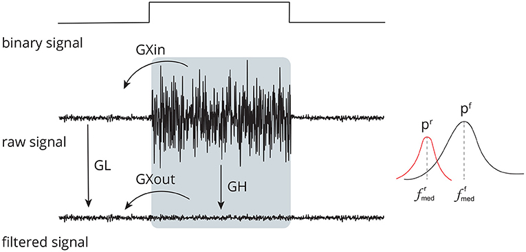
Figure 5. Set of time (GL, GH, GXin, and GXout) and frequency (pr, pf, , and ) domain features used to evaluate the performance of distinct methods for adaptive filtering EEG corrupted by facial EMG. The features compare the signals before and after adaptive filtering and consider the regions in which there is the presence and absence of muscle activity.
Equation (3) defines GL. The general idea is to apply a sliding, non-overlapping 1 s window with 5,000 samples to the data, compute the root-mean-square (RMS) value for each window, and then estimate the median of the RMS values. As the length of the window is 1 s, the number of samples in each window is equal to the sampling frequency fs, which is 5 kHz.
where
corresponds to the median of the RMS values estimated from the signal Xin0, i.e., the non-filtered signal, and
corresponds to the median of the RMS values estimated from the signal Xout0, i.e., the filtered signal, being a set in which each of its values corresponds to a window, the total number of windows, the discrete time in which the window starts, and the discrete time in which the window ends. N is the number of samples of the signal.
GH (Figure 5) is the feature that estimates the ratio between noise-corrupted and filtered signals in an EMG-contaminated region. It is defined in Equation (6). It is calculated in a manner similar to that of GL; hence, equivalent definitions will not be supplied to prevent duplication.
While the GL and GH features evaluate the ratio of signal amplitudes considering different parts of the binary signal, the GXin and GXout features measure the ratio of signal amplitudes comparing regions with and without noise (Figure 5), as given in Equations (7) and (8). The estimates are similar to that of GL and GH, thus they are not provided.
2.3.2. Frequency domain features
For the estimate of the frequency domain features (pr, pf, , and ), first the power spectral density estimate, pxx, of the discrete-time signal was estimated by using the Yule-Walker method. The signal energy was estimated for the frequency f = {0, 0.01, 0.02, ⋯ , fs/2} in Hz, considering a model of order 10. The median frequency and its corresponding energy were estimated from pxx for the non-filtered ( and pr) and filtered ( and pf) signals.
2.4. Statistical analysis
Statistical analysis was performed using R, which is a language and environment for statistical computing (R Core Team, 2021). Considering the studied methods and experimental conditions, the analyses were designed to answer the following research questions: (i) Which facial muscle contributes the most to EEG contamination? (ii) Which decomposition methods are preferable for generating reference signals for adaptive filtering? (iii) Considering its effect on the EEG signal and its components, which adaptive filtering methods are the most desirable?
2.4.1. Characterization of the contamination of the electroencephalogram by distinct facial muscles
Figure 6 depicts the main steps employed to characterize the contamination of EEG by facial muscles. The GL and GH features were used to investigate how distinct facial muscles contaminate EEG signals. By varying the parameter k of the soft-thresholding procedure, from 0.1 to 2.0 with a resolution of 0.1, it is possible to obtain, for each decomposition method, a distinct feature vector for GL and GH. Figure 7 shows typical vectors for the collected signals.
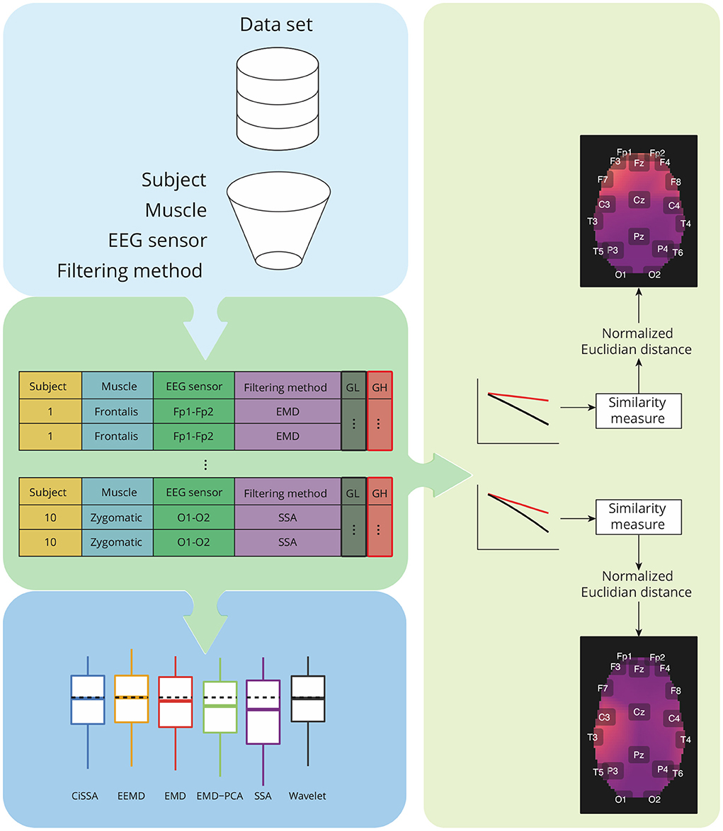
Figure 6. Overview of the analysis required for characterization of contamination caused by different facial muscles, as well as a comparison of the performance of decomposition methods based on the features GH and GL. The analysis takes into account data grouping by participants, muscles, EEG sensors, and filtering methods. For each group, a similarity measure based on the normalized Euclidian distance can be estimated between a pair of vectors representing GH and GL estimates for varying a parameter used in the soft-thresholding of the signal components. The similarity metrics are used to create spatial brain maps that depict the contamination of EMG levels at various areas. Statistical analyses are carried out for GH, GL, and similarity measures.
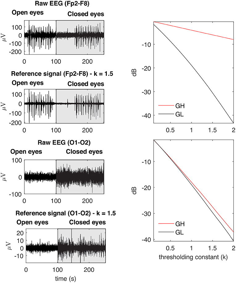
Figure 7. Examples of typical GL and GH feature vectors obtained for high (Fp2–F8) and low (O1-O2) levels of EMG contamination on EEG signals. By decomposing the raw EEG signals with EMD, the reference signals were obtained. The contamination level of the EEG signal can be captured by the distance between the feature vectors, in the sense that an increased distance is related to a lower signal to noise ratio. The examples demonstrate typical collected signals for the open and closed eyes scenarios.
The estimated features, GL and GH, were grouped by subjects, muscles, EEG sensors, and filtering methods. For each pair of feature vectors a similarity measure based on the normalized Euclidian distance was computed (Barrett, 2005). These values of the similarity measures were used to generate a topological map in which the light colors are associated to the contamination of facial EMG on EEG. A customized function was developed in R to generate the topological maps according to the Montreal Neurological Institute (MNI) coordinates mapped to the International 10-20 System (Okamoto et al., 2004).
In addition to the visualization of topological maps, the normalized Euclidean distance between GL and GH were used to quantify the electromyographic contamination produced by distinct muscles. The box plot of the normalized Euclidean distance were computed and the mean of the variables were statistically compared. The statistical analysis was performed considering the scenarios of independence and dependence to the subjects.
To compare the variables, one-way analysis of variance (ANOVA) was used. After fitting the ANOVA model to the data, the model's assumptions were verified, i.e., the evaluation of the homogeneity of variances (Levene's test) and normality of the residuals' distribution (Kolmogorov–Smirnov test). The p-value for all analyses was 0.05. Tukey's honestly significant difference test (Tukey's HSD) was used to examine the significance of differences between sample means. If the variables did not meet the assumptions of ANOVA, the Kruskal–Wallis rank sum test and Dunn's test for multiple comparisons were employed to compare them.
2.4.2. Comparison of the performance of distinct decomposition methods
As seen in Figure 3, the decomposition methods in conjunction with the soft-thresholding procedure act as a filtering method that enables the generation of a suitable reference signal for adaptive filtering. In this regard, it is necessary to preserve EMG regions as much as possible so that adaptive filters can attenuate them appropriately.
The GL and GH measures were used to compare the performance of different decomposition approaches. Based on the definitions of GL (Equation 3) and GH (Equation 6), the most appropriate filtering method is the one that produces the lowest GL and the largest GH, i.e., the method that reduces the signal amplitude in the regions without EMG while preserving the amplitude in the regions of EEG contaminated by EMG as much as possible. For the generation of an appropriate reference signal, a substantially greater reduction of GL relative to GH is expected.
The box plots of GL and GH were generated, and their respective means were compared statistically. For this purpose, the statistical analysis followed the procedure stated previously, which comprised fitting an ANOVA model to the data, validating the method's assumptions, and employing an alternative non-parametric method if ANOVA was not appropriate.
2.4.3. Comparison of the performance of distinct adaptive filtering methods and experimental conditions
2.4.3.1. Evaluation based in time-domain features
The GL, GH, GXin, and GXout features were evaluated for both the EMG (EMGr) and EEG (EEGr) reference signals. GL and GH were used to evaluate the performance of adaptive filtering for each type of reference signal. In contrast to decomposition methods, the appropriate adaptive filtering method should reduce the signal amplitude in regions contaminated by EMG while preserving signal amplitude in regions of EEG without EMG contamination. Therefore, the appropriate adaptive filtering strategy for reducing the influence of EMG on EEG is the one that produces a GL close to zero (to preserve the EEG signal) and GH less than zero (indicating the reduction of EMG contamination).
The feature GXin and GXout were employed to evaluate and compare the behavior of the adaptive filtering in the regions of EEG with and without EMG. The lower the GXout compared to GXin, the greater the attenuation of the EEG regions contaminated by EMG. In addition, the closer to zero is GXout (GXout → 0), the greater the capacity of the adaptive filtering method to preserve the amplitude of the EEG signal in EMG-contaminated regions.
Box plots were used to visually investigate the values of central trend, dispersion and symmetry of the characteristics for each of the scenarios investigated. To verify the differences between the characteristics estimated from different adaptive filtering methods, the means of the variables were compared by ANOVA. If the premises of such a model were not verified, a non-parametric approach was then employed, as previously explained.
2.4.3.2. Evaluation based in frequency-domain features
The non-filtered and filtered EEG signals were decomposed into their fundamental oscillations (Delta, Theta, Alpha, Beta, and Gamma) and box plots for the median frequency and its associated power were calculated. The study took into account the signal regions of the open and closed eye experimental conditions, as well as the overall signal that combines these two regions.
The normality of the variables were verified by the Kolmogorov–Smirnov test (p > 0.05), and then if the variables had a normal distribution the non-paired t-student test (p < 0.05) was applied to verify whether the mean of the variable related to the filtered signal reduced in relation to the non-filtered signal, i.e., the raw signal. If the distribution of the variables were not normal then the non-parametric Mann-Whitney U test was used (p < 0.05). Outliers were removed by eliminating observations that were outside of the following interval [Q1 − 1.5IQR, Q3 + 1.5IQR], in which Q1 is the first quartile, Q3 the third quartile and IQR the interquartile range.
2.4.4. Comparison of execution time of decomposition and adaptive filtering methods
The execution time of the adaptive decomposition and filtering methods were evaluated by the means of the Matlab timeit function. This function performs multiple calls from the routine under analysis and returns the median value of the time measurements. The process for estimating the execution time employed actual and equal data for all methods. The evaluation considers samples with sizes from 25,000 to 1,000,000, with increments of 25,000, i.e., 40 different intervals. For each sample size, eight execution times were estimated to obtain a more representative estimate of the execution time.
The machine that processed the data had the following features: Ryzen 9 5900X 12-core/24-threads @3.7 GHz; RAM 2 × 16 GB DDR4 @ 3200 MHz; video card Asus RTX 3070 8 GB. The Matlab Parallel Computing Toolbox was used to run the applications in parallel, utilizing all of the computer's processors and available memory.
The comparison of execution time was performed by the non-parametric Kruskal–Wallis test (p < 0.05) as the Shapiro–Wilk test confirmed the distribution of the variables were not normal (p < 0.05). The pairwise comparison between variables was performed by the Nemenyi test (p < 0.05).
3. Results
3.1. Typical collected signals
Figure 8 shows typical EMG and EEG signals simultaneously collected during the experimental trials. The EMG bursts were detected by using the procedure described in Figure 4. The number of EMG bursts and their duration are in accordance to the protocol illustrated in Figure 2. The binary signals resulting from the EMG burst detection are plotted together with two typical EEG signals, one for the Fp2-F8 region, which is more contaminated, and the other for the O1-O2 region, which is less contaminated. Note that in the region when the eyes are closed (see the raw EEG: O1-O2) it is possible to see an increase in the amplitude of the EEG signal.
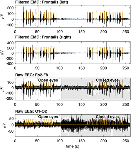
Figure 8. Typical EMG and EEG signals collected during the experimental trials. The EMG signals from the left and right Frontalis are shown. These signals were filtered to remove linear and non-linear trends. The EMG bursts were detected and then the binary signals oscillating from two levels were generated. Simultaneously collected EEG signals are shown for Fp2–F8 (high contamination) and O1-O2 (low contamination) locations. The binary signals are placed over the EEG signals for the indication of the periods in which there was EMG contamination.
3.2. Characterization of the contamination of the EEG by EMG signals
Figures 9, 10 depict topological maps for each subject and activated muscle. The visual inspection of the maps allow us to conclude that the Masseter is the muscle which produced the largest level of contamination, followed by the Frontalis and Zygomatic. These maps suggest also that the contamination and its spread over the brain map is dependent on the subject, which may be related to specific anatomical characteristics of the individual.
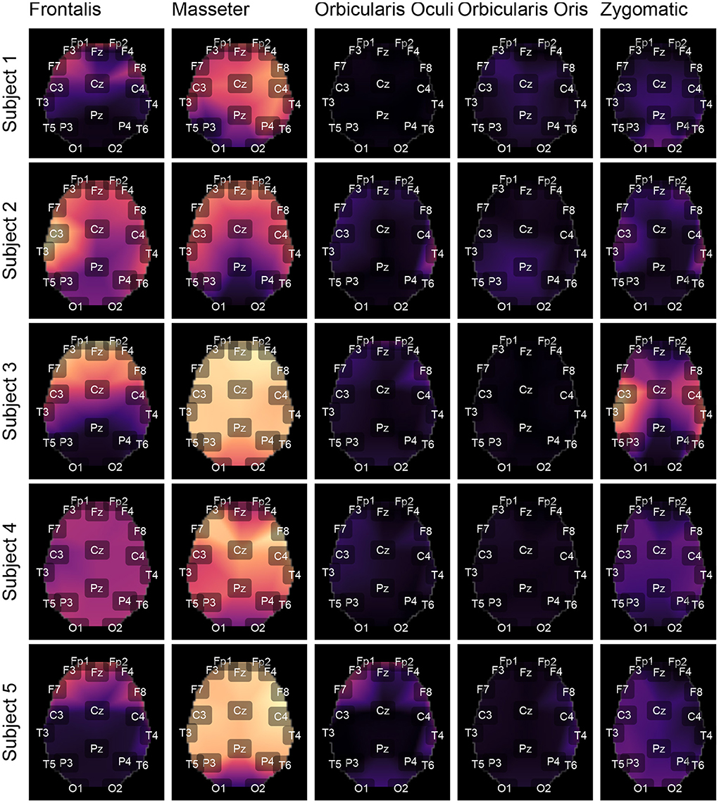
Figure 9. Using the international 10-20 system, the topological maps illustrate how the studied muscles contaminate distinct brain regions. Lighter colors represent the most contaminated locations, whereas darker colors denote the least contaminated areas. The presented results are for subjects from 1 to 5. The colors represent the similarity measure between the GL and GH features.
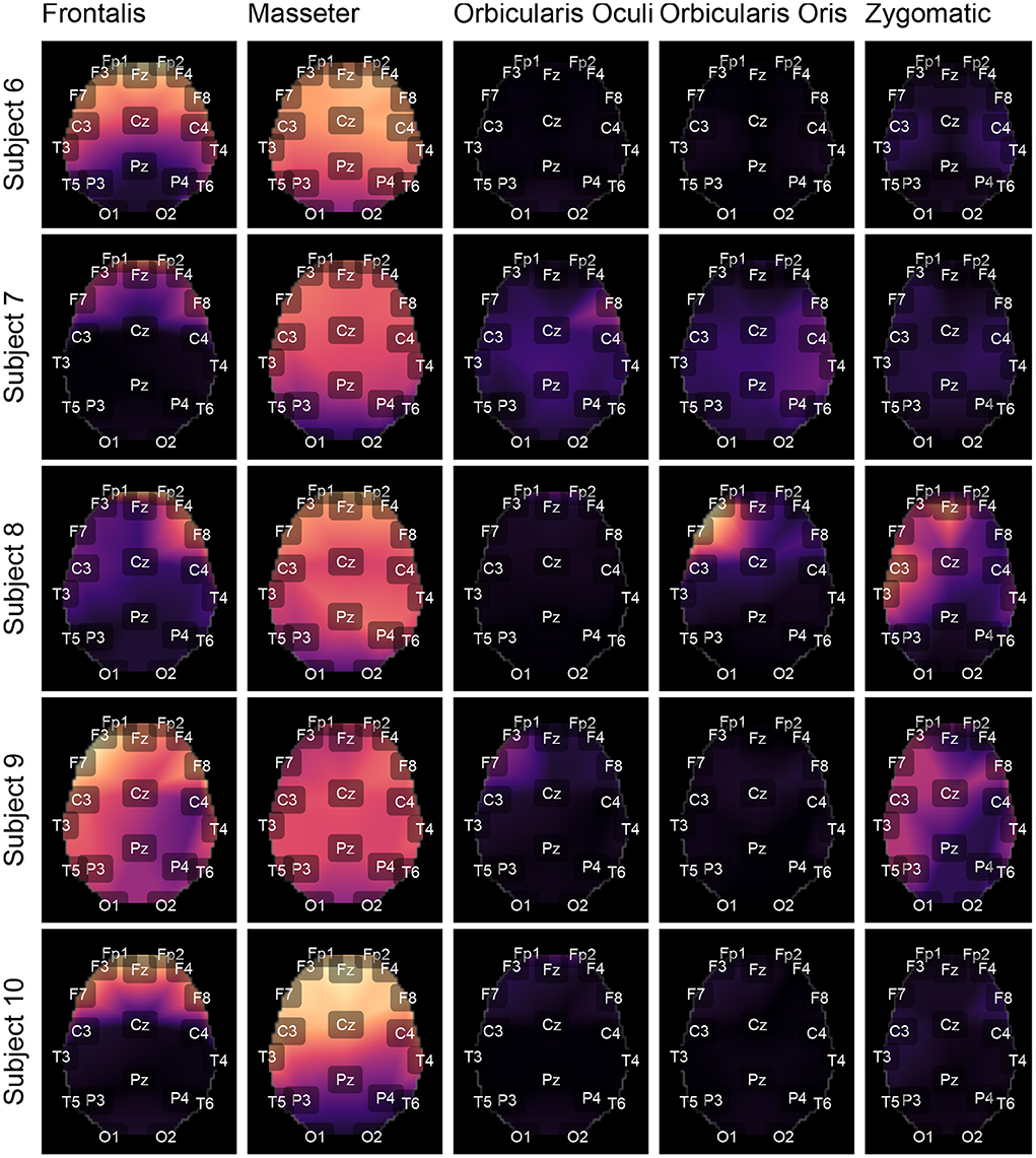
Figure 10. Topological maps for subjects from 6 to 10.
Figure 11 shows typical GL and GH feature vectors estimated for Subject 1. In each graphic six pairs of feature vectors are presented. Each pair of feature vectors was estimated from a specific decomposition method. The behavior of the feature vectors are similar for all subjects. The interpretation of the results is straightforward in the sense that the more similar the GL and GH feature vectors, the less contaminated the EEG signal is. For instance, for the occipital region (O1-O2) there is a high similarity (i.e., low distance) between the feature vectors for nearly all muscles, while for the frontal region (e.g., Fp1-Fp2) the produced contamination is higher for the Frontalis and Masseter. The estimates of feature vectors for the other subjects are available as a Supplementary Figures 2–10.
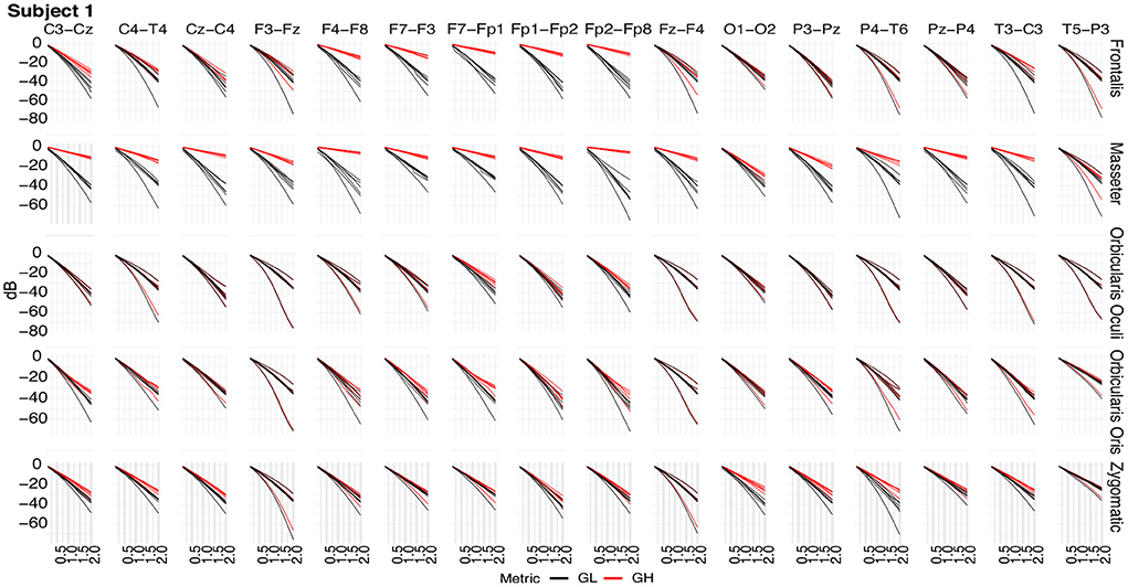
Figure 11. Typical GL and GH feature vectors estimated using different decomposition techniques for Subject 1. Each plot consists of six vector pairs, one pair for each method. The outcomes are presented for individual EEG sensors and muscles.
Box plots of the mean of the normalized Euclidean distance between GL and GH vectors for each muscle are shown in Figures 12C,D. Figure 12C shows results that are independent of subjects and decomposition methods, whereas Figure 12D shows results that are dependent on subjects but independent of decomposition methods.
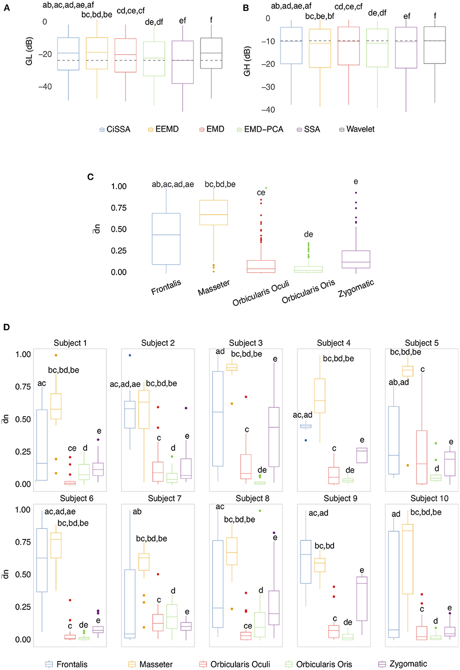
Figure 12. (A) Box plot of GL for distinct decomposition algorithms, regardless of subject and sensor location. The smaller the value of GL, the more appropriate the filtering method. The dashed lines represent the best result obtained with the SSA approach. Statistically significant differences between methods are represented by labels. All possible combinations of two were evaluated. For example, the EEMD method is represented by label “b” and was statistically different from CiSSA (label “a”), EMD (label “c”), EMD-PCA (label “d”), and SSA (label “e”). (B) Box plot of GH for distinct decomposition algorithms, regardless of subject and sensor location. The larger the value of GH the more suitable is the method for filtering. (C) Box plot of the mean normalized Euclidean distance between GL and GH for each muscle, independent of subjects and EEG sensors. The larger the value of this metric, the more contamination is caused by the muscle. (D) Box plot of the mean normalized Euclidean distance between GL and GH for each muscle and subject, independent of the EEG sensor.
The results shown in Figures 12C,D are consistent with those observed in Figures 9, 10 (topological maps). In general, the Masseter was the muscle responsible for the highest EEG signal contamination, followed by the Frontalis and Zygomatic. The Frontalis exhibited the highest level of contamination variability, whereas the Orbicularis Oris produced the least. There was no significant difference between the mean normalized distances estimated from the Orbicularis Oculi and Orbicularis Oris muscles (Figure 12C). Figure 12D shows that a similar result was found for all subjects.
ANOVA could not be employed for the statistical analysis since its assumptions were violated. To compare the variables, the Kruskal–Wallis rank sum test and Dunn's test for multiple comparisons were used in all analyses.
3.3. Evaluation of decomposition methods to generate reference signals for adaptive filtering
In Figures 12A,B, the box plots of GL and GH are presented for each decomposition method, independently of subject and brain area. From the box plots, it is possible to compare and contrast the distributions of feature vectors for each investigated method. For GL the dashed lines indicate the median of the method which produces the largest amplitude reduction in the regions in which there is no EMG contamination. SSA was the most appropriate method among those considered.
For GH, the dashed lines represent the median of the approach that yields the lowest amplitude reduction in EMG-contaminated locations. Wavelet was the most appropriate method among those studied. In general, when both metrics, GL and GH, are considered, SSA is the most appropriate because it reduces the signal amplitude in regions without EMG contamination the most, while preserving the regions contaminated by EMG in a satisfactory manner, allowing the generation of an appropriate reference signal for adaptive filters. There was no statistically significant difference between the EEMD and Wavelet methods for GL (Figure 12A). There were no significant differences between CiSSA and EMD, and EEMD and EMD-PCA for GH (Figure 12B).
3.4. Evaluation of the filtering based on the time-domain features
Figure 13 depicts the overall behavior of distinct adaptive filtering methods according to the time-domain features and type of reference signals (EEG or EMG). In general, all adaptive filtering methods were capable of filtering EMG contamination from EEG. As can be seen in Figures 13B,D, the medians of GH are less than zero, confirming, thus, that the EMG contamination was attenuated. On the other hand, when evaluating the preservation of regions of EEG without EMG, the results vary, depending on the type of reference. Ideally the median of GL should be as close to zero as possible. When the reference signal is the EEG, the most appropriate method is the RLS as it causes the lowest changes in the regions of EEG without EMG contamination. When the reference is the EMG signal, the most appropriate methods were the NLMS and Wiener.
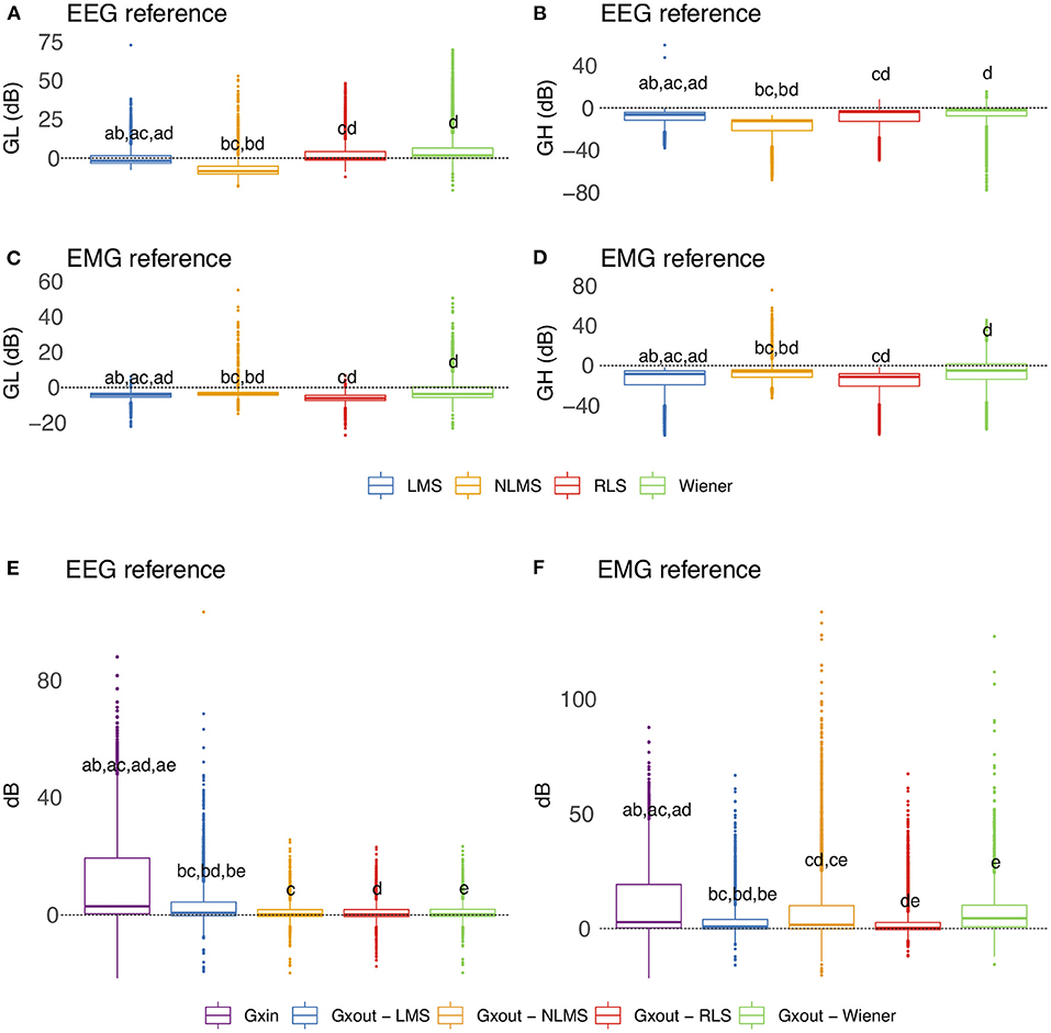
Figure 13. Evaluation of distinct adaptive filtering methods based on the time-domain features. The assessment is independent of the decomposition method and specific to the type of reference signal. (A–D) show results referent to GH and GL. (E,F) Present the results related to GXin and GXout.
Figures 13E,F show the behavior of the variables GXin and GXout for adaptive filtering. For the EEG reference, the obtained results confirm the attenuation of the EMG signal, as all the medians of Xout are lower than the median of GXin. On the other hand, for the EMG reference, the results yielded by the Wiener filter were not satisfactory.
Considering the time-domain features, the EEG reference signal was more appropriate for the adaptive filtering, as it allowed for the preservation of EEG regions not contaminated by EMG. Furthermore, when evaluating the variables GXin and GXout it is clear that when using the EEG as a reference, the filtered EMG-contaminated region will preserve the EEG activity. Figure 14 shows an example of EMG-corrupted EEG and its filtered version. The figure insets show the effect of the adaptive filtering, in which the EMG amplitude is attenuated and the EEG activity in the EMG-contaminated region follows the EEG dynamics of the EEG signal in the neighbor regions in which there are no EMG contamination.
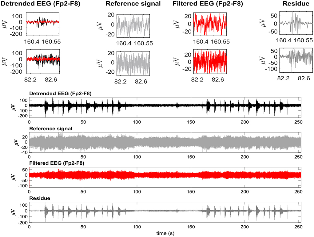
Figure 14. A typical EEG signal corrupted by facial EMG. The EEG signal is from the Fp2-F8 region because it is most affected by facial electromyography. EMG bursts can be seen on the detrended EEG signal. The EEG signal was used as a reference signal, estimated from EMD, and then filtered using the RLS filter. The residue, which is the difference between the detrended and filtered EEG data, clearly shows the EMG activity that was eliminated from the signal. The inset plots at the top indicate the selection of two EEG regions contaminated by EMG. The filtered signal is shown over the contaminated signal in red. For each region, the detrended EEG, reference signal, filtered EEG, and residue are shown.
3.5. Evaluation of the filtering based on the frequency domain features
The box plots in Figure 15 show the behavior of the median frequency and its power for the EEG signal together with its components, i.e., Delta (0.5–4 Hz), Theta (4–7 Hz), Alpha (7–13), Beta (13–30), and Gamma (30–70 Hz). The results contrast the raw non-filtered signal with the filtered signal. The non-parametric Mann-Whitney U test was used as the distributions of the variables were not normal (p < 0.05).
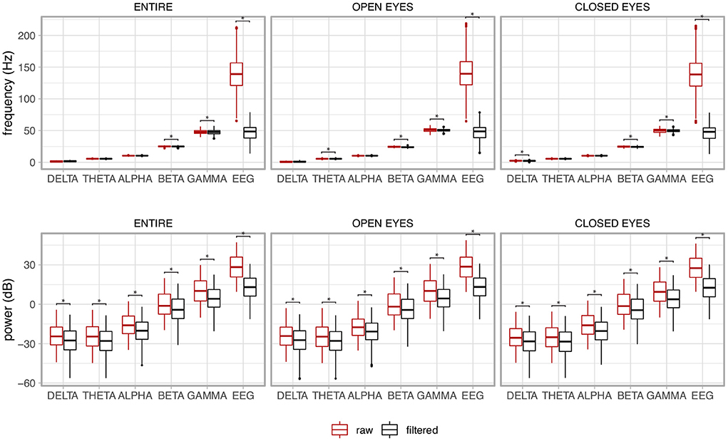
Figure 15. Median frequency and its power of the electroencephalogram (EEG) together with its components for the whole signal (ENTIRE) and the two experimental conditions (OPEN EYES and CLOSED EYES). A contrast between the raw non-filtered signal with the filtered signal is presented. The asterisks show the pair of variables in which the variable associated to the filtered signal was significantly reduced in comparison to the non-filtered signal, i.e., raw signal.
There is a clear drop in the frequency and power of the EEG signal resulting from the filtering. As expected, the power of the signal is reduced for all components although their median frequencies are kept in the expected frequency band. The same behavior is noted for the experimental conditions of open and closed eyes, and for the whole signal, which considers the joint analysis of the open and closed eye regions.
3.6. Execution time of decomposition and adaptive filtering methods
Figure 16 depicts the typical execution times for all methods investigated. The estimates in A and B are based on the mean of the eight execution times for each sample size. The linear relationship between sample size and execution time may indicate that the methods have linear computational complexity, O(n).
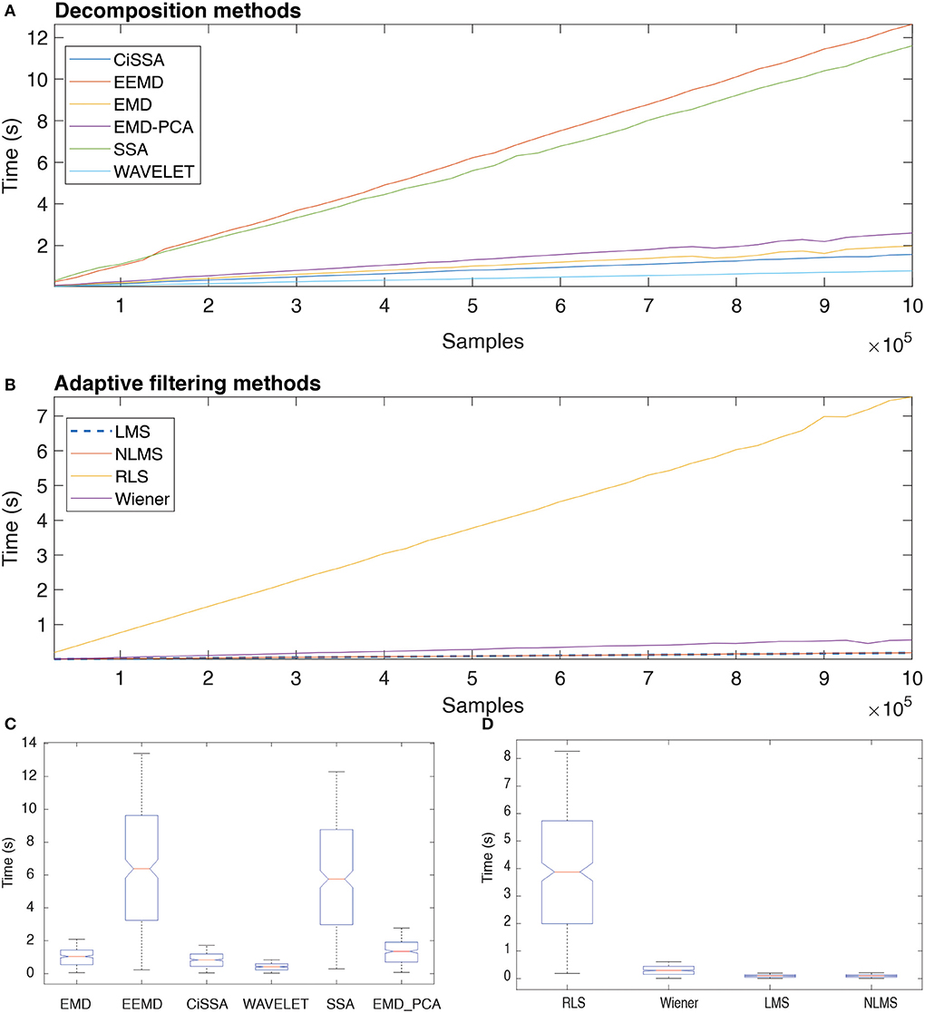
Figure 16. Execution time of distinct decomposition (A) and adaptive filtering (B) methods as function of the number of samples. The box plots show the central trend and dispersion of execution times (C,D).
According to the results in Figure 16C, the execution times for EEMD and SSA are statistically equivalent (Nemenyi Test, p > 0.05), just as they are for EMD and CiSSA. Wavelet obtained the shortest execution time. According to the results in Figure 16D, the execution times for LMS and NLMS are statistically equivalent. Furthermore, RLS has a significantly longer execution time than the others.
4. Discussion
The filtering approach depicted in Figure 3 has been proposed for the removal of facial muscular artifacts from EEG signals, which is an important requirement for distinct applications. It is a single channel approach for filtering low SNR EEG signals. In general, the proposed method is based on a hybrid filtering approach, combining adaptive filters with decomposition techniques. Thus, in this research, the performance of several decomposition (EMD, EEMD, CiSSA, Wavelet, SSA, and EMD-PCA) and optimal filtering (RLS, Wiener, LMS, and NMLS) methods were evaluated.
Although it is possible to find some databases containing EEG signals corrupted by EMG, we could not find any open data set similar to the one that was collected in this research. The relevance of the collected data set is that it considers the influence of the activity of several facial muscles to the contamination of EEG signals. The experimental protocol was carefully designed to take into consideration data collection in practical scenarios, such as the execution of facial expressions commonly used for some human-computer interfaces based on facial EMG (Andrade et al., 2013). In addition, all EEG signals were collected simultaneously with EMG signals guaranteeing the necessary synchronization between signals and the possibility of annotating the regions in which EEG signals were actually contaminated by EMG. The dataset included a total of 2,250 s of EEG signals corrupted by EMG, with the participation of 10 subjects and distinct experimental conditions (e.g., open and closed eyes, EMG bursts of varying durations, and the activation of different facial muscles), allowing for the required variability to test the performance of filtering methods.
Other decomposition and adaptive filtering methods can be added to the filter architecture of the EEG single channel filtering approach depicted in Figure 3 without altering the entire filtering strategy. This is an interesting feature for the development of computational libraries that can benefit from the use of encapsulated code implementing decomposition and adaptive filtering methods that can be directly plugged into the general steps, i.e., the processing pipe depicted in Figure 3. To aid in the diffusion of this architecture, the authors of this paper have made available all Matlab and R scripts at https://doi.org/10.5281/zenodo.6591866. In addition, sample data and demonstration scripts are provided to facilitate comprehension and replication of the filtering approach presented and evaluated in this study.
In this study, the detection of EMG bursts is relevant because these bursts mark the regions contaminated and non-contaminated by electromyography automatically. The identification of these regions are used in the stage of soft-thresholding signal components and for computing the proposed set of features to measure the performance of filtering methods. We decided not to detect the bursts directly from the EEG contaminated signal to guarantee that the noise present in the EEG signal was really from the EMG activity. However, the use of the proposed filtering approach (Figure 3) can be applied without the simultaneously collection of EMG signals. If this is the case, it would be necessary to detect EMG bursts directly from the EMG-corrupted EEG.
The time and frequency domain features proposed in this work (Figure 5) were advantageous for the characterization of facial EMG contamination on the EEG. Figures 9, 10 depict an approach for energy visualization of topological maps displaying the degree of contamination created by distinct muscles based on this set of characteristics. Utilizing the normalized Euclidean distance as a measure of similarity allowed for the visual, qualitative, and quantitative comparison of topological maps estimated for various subjects and active muscles.
As indicated in Figure 3 an important step for adaptive filtering is the generation of reliable reference signals. In the proposed approach the reference signal is generated from the application of soft-thresholding to the signal components. To evaluate the performance of distinct decomposition methods the GL and GH metrics were proposed. These metrics were also employed to characterize the EMG contamination in distinct regions of the scalp (Figures 9, 10). An interesting aspect of the contamination is that although there is a general pattern, e.g., muscles such as the Frontalis and Masseter contributed more to the EEG contamination, the way this contamination spread over the scalp is specific to the individual. This fact can be verified by the relatively large variability of the variables presented in Figures 12C,D.
According to the findings (Figures 9, 10, 12), the Masseter muscle provided the highest degree of contamination, followed by the Frontalis and Zygomatic. Variability between individuals was an important component of this study; for example, the Orbicularis Oris of subject 8 produced a substantial contamination of the EEG obtained in the frontal region. This may involve anatomical and behavioral characteristics of the individual. This requires that EEG filtering methods be devised to accommodate data variations introduced by anatomical, physiological, and experimental settings. This also justifies the more sophisticated experimental methodology utilized in this study.
In general, all decomposition methods investigated in this study were suitable for generating adequate adaptive filtering reference signals. Nonetheless, we believe that the SSA method is superior because it successfully preserved EEG in non-contaminated regions while lowering the signal amplitude in EMG-contaminated regions significantly (Figures 12A,B). Considering the type of signal reference (EMG or EEG) the results reported in Figure 13 suggest that the reference based on the EEG signal is preferable because of the lower variability exhibited (Figures 13E,F) when compared to the EMG reference.
This study also investigated various adaptive filtering algorithms (LMS, NLMS, RLS, and Wiener) to reduce electromyographic activity as much as possible in EEG data heavily contaminated by EMG. When using the EEG as a reference signal, RLS and NLMS were the best methods among those tested. In general, these methods best ensured: (i) attenuation of electromyographic activity in regions of EMG-contaminated EEG (Figure 13B), (ii) preservation of electroencephalographic activity in regions of EEG without EMG (Figure 13A), and (iii) the dynamics of the resulting signal, not mischaracterizing the EEG signal over time (Figures 13, 14). However, when the reference signal was the EMG, the LMS, and RLS algorithms performed best. Thus, the RLS method is the most preferred, as it produced satisfactory results regardless of the type of reference signal.
The results shown in Figure 15 confirm that the single channel approach proposed in this research was capable of reducing EMG contamination on the EEG signals, while preserving relevant information of the electroencephalogram. For instance, typical values of frequency were found for each EEG component. In addition, there was reduction in the power of the non-filtered EEG signal compared to its filtered version, and this could also be observed for each EEG component.
The results presented in Figure 16 reveal that there is a linear relationship between the number of samples, i.e., signal length, and the execution time required to process the data. This suggests that the decomposition and filtering algorithms have a linear computational complexity. In total, 90 h were spent processing the entire data set of this investigation, taking into account the processing time for ten subjects and all experimental conditions. Methods that need less time to process data are desirable in this regard, even if they do not produce optimal results.
In future research, the proposed method could be utilized to reduce interference produced by electromyography in applications controlled by electroencephalographic activity (such as brain-computer interfaces). Furthermore, while this study only involves healthy people, we encourage the examination and confirmation of the technique created for people with disorders like amyotrophic lateral sclerosis. This would allow for the creation of more robust assistive technology as well as a better understanding of the electroencephalographic activity associated with this type of clinical condition.
5. Conclusion
This study introduced a single-channel filtering method for reducing facial electromyography from EEG signals. The proposed method is sufficiently general to accommodate multiple decomposition and adaptive filtering techniques within a single architecture.
Using a data set that enabled the generation of EMG-corrupted EEG in experiments involving facial muscular activation, the filtering method was evaluated. The set of time and frequency domain characteristics enabled the visualization and quantification of facial EMG contamination of the EEG. This set of features allowed for comparative analysis of filtering methods.
The results indicated that the Masseter was the muscle that contaminated the EEG the most; however, individual variation should not be disregarded, as the contraction of other facial muscles in some people may generate significant contamination on EEG signals.
In general, all investigated decomposition and adaptive filtering methods effectively filtered facial EMG-corrupted EEG; however, the decomposition method SSA reduced EMG contamination while preserving the EEG signal more. This method's relative slowness in comparison to other studies is its most significant drawback. In terms of the adaptive filtering method, it was observed that the reference signal (EMG or EEG) affects the method's performance, despite the methods' similarities.
Data availability statement
The datasets presented in this article are not readily available because, the set of features can be shared, but no the raw data, as this is not allowed by the Brazilian regulations. Requests to access the datasets should be directed to https://doi.org/10.5281/zenodo.6591866.
Ethics statement
This study follows the Resolution 466/2012 of the National Health Council. The study was conducted at the Centre for Innovation and Technology Assessment in Health of the Federal University of Uberlândia (UFU), Brazil. The protocols were approved by the Human Research Ethics Committee (CEP-UFU), CAAE Number: 43670815.4.0000.5152. The patients/participants provided their written informed consent to participate in this study. Written informed consent was obtained from the individual(s) for the publication of any potentially identifiable images or data included in this article.
Author contributions
All authors listed have made a substantial, direct, and intellectual contribution to the work and approved it for publication.
Funding
The present work was carried out with the support of the National Council for Scientific and Technological Development (CNPq), Coordination for the Improvement of Higher Education Personnel (CAPES—Program CAPES/ DFATD-88887.159028/ 2017-00, Program CAPES/ COFECUB-88881.370894/ 2019-01, and Program CAPES-PRINT-UFU) and the Foundation for Research Support of the State of Minas Gerais. AO is fellow of CNPq, Brazil (304818/2018-6 and 305223/2014-3). MV is fellow of CNPq, Brazil (304533/2020-3). AP is fellow of CNPq, Brazil (309525/2021-7).
Acknowledgments
The authors are grateful to the volunteers who contributed to this research.
Conflict of interest
The authors declare that the research was conducted in the absence of any commercial or financial relationships that could be construed as a potential conflict of interest.
Publisher's note
All claims expressed in this article are solely those of the authors and do not necessarily represent those of their affiliated organizations, or those of the publisher, the editors and the reviewers. Any product that may be evaluated in this article, or claim that may be made by its manufacturer, is not guaranteed or endorsed by the publisher.
Supplementary material
The Supplementary Material for this article can be found online at: https://www.frontiersin.org/articles/10.3389/fncom.2022.822987/full#supplementary-material
References
Abo-Zahhad, M., Ahmed, S. M., and Abbas, S. N. (2015). A new EEG acquisition protocol for biometric identification using eye blinking signals. Int. J. Intell. Syst. Appl. 7, 48–54. doi: 10.5815/ijisa.2015.06.05
Alam, M. E., and Samanta, B. (2017). “Performance evaluation of empirical mode decomposition for EEG artifact removal,” in Volume 4B: Dynamics, Vibration, and Control (Tampa, Florida: American Society of Mechanical Engineers), 1–8. doi: 10.1115/IMECE2017-71647
Albera, L., Kachenoura, A., Comon, P., Karfoul, A., Wendling, F., Senhadji, L., et al. (2012). ICA-based EEG denoising: a comparative analysis of fifteen methods. Bull. Pol. Acad. Sci. 60, 407–418. doi: 10.2478/v10175-012-0052-3
Andrade, A. O., Nasuto, S., Kyberd, P., Sweeney-Reed, C. M., and Kanijn, F. V. (2006). EMG signal filtering based on empirical mode decomposition. Biomed. Signal Process. Control 1, 44–55. doi: 10.1016/j.bspc.2006.03.003
Andrade, A. O., Pereira, A. A., Pinheiro, C. G. Jr, and Kyberd, P. J. (2013). Mouse emulation based on facial electromyogram. Biomed. Signal Process. Control 8, 142–152. doi: 10.1016/j.bspc.2012.09.001
Barrett, P. (2005). Euclidean Distance: Raw, Normalized, and Double-Scaled Coefficients. The Technical Whitepaper Series 6. Available online at: https://www.pbarrett.net/techpapers/euclid.pdf
Bógalo, J., Poncela, P., and Senra, E. (2021). Circulant singular spectrum analysis: a new automated procedure for signal extraction. Signal Process. 179:107824. doi: 10.1016/j.sigpro.2020.107824
Bono, V., Das, S., Jamal, W., and Maharatna, K. (2016). Hybrid wavelet and EMD/ICA approach for artifact suppression in pervasive EEG. J. Neurosci. Methods 267, 89–107. doi: 10.1016/j.jneumeth.2016.04.006
Castellanos, N. P., and Makarov, V. A. (2006). Recovering EEG brain signals: Artifact suppression with wavelet enhanced independent component analysis. J. Neurosci. Methods 158, 300–312. doi: 10.1016/j.jneumeth.2006.05.033
Chen, X., He, C., and Peng, H. (2014). Removal of muscle artifacts from single-channel EEG based on ensemble empirical mode decomposition and multiset canonical correlation analysis. J. Appl. Math. 2014:261347. doi: 10.1155/2014/261347
Chen, X., Liu, A., Chiang, J., Wang, Z. J., McKeown, M. J., and Ward, R. K. (2016). Removing muscle artifacts from EEG data: multichannel or single-channel techniques? IEEE Sensors J. 16, 1986–1997. doi: 10.1109/JSEN.2015.2506982
Correa, A. G., Laciar, E., Pati no, H. D., and Valentinuzzi, M. E. (2007). Artifact removal from EEG signals using adaptive filters in cascade. J. Phys. 90:012081. doi: 10.1088/1742-6596/90/1/012081
Daly, I., Scherer, R., Billinger, M., and Muller-Putz, G. (2015). FORCe: fully online and automated artifact removal for brain-computer interfacing. IEEE Trans. Neural Syst. Rehabil. Eng. 23, 725–736. doi: 10.1109/TNSRE.2014.2346621
Diniz, P. S. R. (2008). Adaptive Filtering. Springer New York, NY: Springer US. doi: 10.1007/978-0-387-68606-6
Farhang-Boroujeny, B. (1999). Adaptive Filters Theory and Applications. West Sussex, United Kingdom: Wiley.
Ferdous, J., and Ali, S. (2017). A comparison of wiener and Kalman filters for the artifact suppression from EEG signal. Int. J. Sci. Res. 6, 2029–2035. doi: 10.21275/ART20172896
Foxe, J. J., and Snyder, A. C. (2011). The role of alpha-band brain oscillations as a sensory suppression mechanism during selective attention. Front. Psychol. 2:154. doi: 10.3389/fpsyg.2011.00154
Frølich, L., and Dowding, I. (2018). Removal of muscular artifacts in EEG signals: a comparison of linear decomposition methods. Brain Inform. 5, 13–22. doi: 10.1007/s40708-017-0074-6
Gabsteiger, F., Leutheuser, H., Reis, P., Lochmann, M., and Eskofier, B. M. (2014). “ICA-based reduction of electromyogenic artifacts in EEG data: comparison with and without EMG data,” in 2014 36th Annual International Conference of the IEEE Engineering in Medicine and Biology Society (Chicago, IL, USA). doi: 10.1109/EMBC.2014.6944466
Gao, J., Sultan, H., Hu, J., and Tung, W.-W. (2010). Denoising nonlinear time series by adaptive filtering and wavelet shrinkage: a comparison. IEEE Signal Process. Lett. 17, 237–240. doi: 10.1109/LSP.2009.2037773
Gaur, P., Pachori, R. B., Wang, H., and Prasad, G. (2015). “An empirical mode decomposition based filtering method for classification of motor-imagery EEG signals for enhancing brain-computer interface,” in 2015 International Joint Conference on Neural Networks (IJCNN) (Killarney, Ireland). doi: 10.1109/IJCNN.2015.7280754
Gerardo, J., Sanchez, J. C., and Velazquez, J. (2011). “Applications of adaptive filtering,” in Adaptive Filtering Applications, eds L. Garcia (Rijeka, Croatia: InTech), 1–20. doi: 10.5772/16873
Goncharova, I., McFarland, D., Vaughan, T., and Wolpaw, J. (2003). EMG contamination of EEG: spectral and topographical characteristics. Clin. Neurophysiol. 114, 1580–1593. doi: 10.1016/S1388-2457(03)00093-2
Hero, A. (2006). Signal processing identity [president's message]. IEEE Signal Process. Mag. 23:4. doi: 10.1109/MSP.2006.1657808
Huang, N. E., Shen, Z., Long, S. R., Wu, M. C., Shih, H. H., Zheng, Q., et al. (1998). The empirical mode decomposition and the Hilbert spectrum for nonlinear and non-stationary time series analysis. Proc. R. Soc. Lond. Ser. A 454, 903–995. doi: 10.1098/rspa.1998.0193
Iyer, D., and Zouridakis, G. (2007). Single-trial evoked potential estimation: comparison between independent component analysis and wavelet denoising. Clin. Neurophysiol. 118, 495–504. doi: 10.1016/j.clinph.2006.10.024
James, C. J., and Hesse, C. W. (2004). Independent component analysis for biomedical signals. Physiol. Measure. 26, R15–R39. doi: 10.1088/0967-3334/26/1/R02
Kher, R., and Gandhi, R. (2016). “Adaptive filtering based artifact removal from electroencephalogram (EEG) signals,” in 2016 International Conference on Communication and Signal Processing (ICCSP) (Melmaruvathur, India). doi: 10.1109/ICCSP.2016.7754202
Kim, M., and Kim, S.-P. (2018). “A comparsion of artifact rejection methods for a BCI using event related potentials,” in 2018 6th International Conference on Brain-Computer Interface (BCI) (Gangwon, Korea (South)). doi: 10.1109/IWW-BCI.2018.8311530
Krishnaveni, V., Jayaraman, S., Anitha, L., and Ramadoss, K. (2006). Removal of ocular artifacts from EEG using adaptive thresholding of wavelet coefficients. J. Neural Eng. 3, 338–346. doi: 10.1088/1741-2560/3/4/011
Kutluay, E., and Kalamangalam, G. P. (2019). Montages for noninvasive EEG recording. J. Clin. Neurophysiol. 36, 330–336. doi: 10.1097/WNP.0000000000000546
Maki, H., Toda, T., Sakti, S., Neubig, G., and Nakamura, S. (2015). “EEG signal enhancement using multi-channel wiener filter with a spatial correlation prior,” in 2015 IEEE International Conference on Acoustics, Speech and Signal Processing (ICASSP) (South Brisbane, QLD, Australia). doi: 10.1109/ICASSP.2015.7178449
Mamun, M., Al-Kadi, M., and Marufuzzaman, M. (2013). Effectiveness of wavelet denoising on electroencephalogram signals. J. Appl. Res. Technol. 11, 156–160. doi: 10.1016/S1665-6423(13)71524-4
Mannan, M. M. N., Jeong, M. Y., and Kamran, M. A. (2016). Hybrid ICA-regression: automatic identification and removal of ocular artifacts from electroencephalographic signals. Front. Hum. Neurosci. 10:193. doi: 10.3389/fnhum.2016.00193
McMenamin, B. W., Shackman, A. J., Greischar, L. L., and Davidson, R. J. (2011). Electromyogenic artifacts and electroencephalographic inferences revisited. NeuroImage 54, 4–9. doi: 10.1016/j.neuroimage.2010.07.057
Mihajlovic, V., Grundlehner, B., Vullers, R., and Penders, J. (2015). Wearable, wireless EEG solutions in daily life applications: what are we missing? IEEE J. Biomed. Health Informatics 19, 6–21. doi: 10.1109/JBHI.2014.2328317
Morbidi, F., Garulli, A., Prattichizzo, D., Rizzo, C., and Rossi, S. (2008). Application of Kalman filter to remove TMS-induced artifacts from EEG recordings. IEEE Trans. Control Syst. Technol. 16, 1360–1366. doi: 10.1109/TCST.2008.921814
Mucarquer, J. A., Prado, P., Escobar, M.-J., El-Deredy, W., and Zanartu, M. (2020). Improving EEG muscle artifact removal with an EMG array. IEEE Trans. Instrum. Measure. 69, 815–824. doi: 10.1109/TIM.2019.2906967
Ngoc, P. P., Hai, V. D., Bach, N. C., and Binh, P. V. (2015). “EEG signal analysis and artifact removal by wavelet transform,” in IFMBE Proceedings (Cham: Springer International Publishing), 179–183. doi: 10.1007/978-3-319-11776-8_44
Nunez, P. L., and Srinivasan, R. (2006). Electric Fields of the Brain. New York: Oxford University Press. doi: 10.1093/acprof:oso/9780195050387.001.0001
Okamoto, M., Dan, H., Sakamoto, K., Takeo, K., Shimizu, K., Kohno, S., et al. (2004). Three-dimensional probabilistic anatomical cranio-cerebral correlation via the international 10–20 system oriented for transcranial functional brain mapping. NeuroImage 21, 99–111. doi: 10.1016/j.neuroimage.2003.08.026
Pivik, R. T., Broughton, R. J., Coppola, R., Davidson, R. J., Fox, N., and Nuwer, M. R. (1993). Guidelines for the recording and quantitative analysis of electroencephalographic activity in research contexts. Psychophysiology 30, 547–558. doi: 10.1111/j.1469-8986.1993.tb02081.x
R Core Team (2021). R: A Language and Environment for Statistical Computing. Vienna: R Foundation for Statistical Computing.
Ramadan, R. A., and Vasilakos, A. V. (2017). Brain computer interface: control signals review. Neurocomputing 223, 26–44. doi: 10.1016/j.neucom.2016.10.024
Rutledge, D., and Bouveresse, D. J.-R. (2013). Independent components analysis with the JADE algorithm. Trends Anal. Chem. 50, 22–32. doi: 10.1016/j.trac.2013.03.013
Safieddine, D., Kachenoura, A., Albera, L., Birot, G., Karfoul, A., Pasnicu, A., et al. (2012). Removal of muscle artifact from EEG data: comparison between stochastic (ICA and CCA) and deterministic (EMD and wavelet-based) approaches. EURASIP J. Adv. Signal Process. 2012:127. doi: 10.1186/1687-6180-2012-127
Salsabili, S., Sardoui, S. H., and Shamsollahi, M. B. (2015). “Interictal EEG denoising using independent component analysis and empirical mode decomposition,” in 2015 38th International Conference on Telecommunications and Signal Processing (TSP) (Prague, Czech Republic). doi: 10.1109/TSP.2015.7296475
Sengupta, S. K., and Kay, S. M. (1995). Fundamentals of statistical signal processing: estimation theory. Technometrics 37:465. doi: 10.2307/1269750
Sweeney, K. (2013). Motion artifact processing techniques for physiological signals (Ph.D. thesis). Faculty of Science and Engineering, Department of Electronic Engineering, National University of Ireland, Maynooth, Ireland.
Sweeney, K. T., Ward, T. E., and McLoone, S. F. (2012). Artifact removal in physiological signals practices and possibilities. IEEE Trans. Inform. Technol. Biomed. 16, 488–500. doi: 10.1109/TITB.2012.2188536
Sweeney-Reed, C. M., Nasuto, S. J., Vieira, M. F., and Andrade, A. O. (2018). Empirical mode decomposition and its extensions applied to EEG analysis: a review. Adv. Data Sci. Adapt. Anal. 10:1840001. doi: 10.1142/S2424922X18400016
Tatum, W. O., Dworetzky, B. A., and Schomer, D. L. (2011). Artifact and recording concepts in EEG. J. Clin. Neurophysiol. 28, 252–263. doi: 10.1097/WNP.0b013e31821c3c93
Turnip, A., and Pardede, J. (2017). Artefacts removal of EEG signals with wavelet denoising. MATEC Web Conf. 135:00058. doi: 10.1051/matecconf/201713500058
Upadhyay, R., Padhy, P., and Kankar, P. (2016). EEG artifact removal and noise suppression by discrete orthonormal s-transform denoising. Comput. Electr. Eng. 53, 125–142. doi: 10.1016/j.compeleceng.2016.05.015
Urigüen, J. A., and Garcia-Zapirain, B. (2015). EEG artifact removal state-of-the-art and guidelines. J. Neural Eng. 12:031001. doi: 10.1088/1741-2560/12/3/031001
Wu, Z., and Huang, N. E. (2009). Ensemble empirical mode decomposition: a noise-assisted data analysis method. Adv. Adapt. Data Anal. 1, 1–41. doi: 10.1142/S1793536909000047
Keywords: EEG, EMG, adaptive filtering, signal decomposition, facial electromyography
Citation: Queiroz CMM, Silva GM, Walter S, Peres LB, Luiz LMD, Costa SC, Faria KC, Pereira AA, Vieira MF, Cabral AM and Andrade AO (2022) Single channel approach for filtering electroencephalographic signals strongly contaminated with facial electromyography. Front. Comput. Neurosci. 16:822987. doi: 10.3389/fncom.2022.822987
Received: 26 November 2021; Accepted: 01 July 2022;
Published: 26 July 2022.
Edited by:
Md. Kafiul Islam, Independent University, BangladeshReviewed by:
Rajesh Kumar Tripathy, Birla Institute of Technology and Science, IndiaAmir Rastegarnia, Malayer University, Iran
Copyright © 2022 Queiroz, da Silva, Walter, Peres, Luiz, Costa, de Faria, Pereira, Vieira, Cabral and Andrade. This is an open-access article distributed under the terms of the Creative Commons Attribution License (CC BY). The use, distribution or reproduction in other forums is permitted, provided the original author(s) and the copyright owner(s) are credited and that the original publication in this journal is cited, in accordance with accepted academic practice. No use, distribution or reproduction is permitted which does not comply with these terms.
*Correspondence: Steffen Walter, steffen.walter@uni-ulm.de