Malware propagation model of fractional order, optimal control strategy and simulations

Zhou, Ying; Liu, Ban-Teng; Zhou, Kai; Shen, Shou-Feng

doi:10.3389/fphy.2023.1201053

ORIGINAL RESEARCH article

Front. Phys., 08 June 2023
Sec. Mathematical Physics
Volume 11 - 2023 | https://doi.org/10.3389/fphy.2023.1201053

Malware propagation model of fractional order, optimal control strategy and simulations

Ying Zhou¹

Ban-Teng Liu¹

Kai Zhou²

Shou-Feng Shen²*

¹College of Information Engineering, Zhejiang Shuren University, Hangzhou, China
²Department of Applied Mathematics, Zhejiang University of Technology, Hangzhou, China

In this paper, an improved SEIR model of fractional order is investigated to describe the behavior of malware propagation in the wireless sensor network. Firstly, the malware propagation model of fractional order is established based on the classical SEIR epidemic theory, the basic reproductive number is obtained by the next-generation method and the stability condition of the model is also analyzed. Then, the inverse approach for the uncertainty propagation based on the discrete element method and least square algorithm is presented to determine the unknown parameters of the propagation process. Finally, the optimal control strategy is also discussed based on the adaptive model. Simulation results show the proposed model works better than the propagation model of integer order. The error of proposed model is smaller than integer order models.

1 Introduction

Wireless sensor network (WSN) is a distributed communication system, which is composed of a large number of sensor nodes with wireless communication and sensing capabilities [1]. Nowadays, WSN is widely applied to build decision support system to overcome many difficult problems in the real world, such as transport, medical, military and so on. However, due to the limited resource in battery energy and low radio bandwidth condition, WSN is always an easy target of many malware attacks, and the nodes in WSN can easily fall victim to some of malware attacks [2, 3]. WSNs are vulnerable to malware attacks because the nodes are typically small, have limited battery power, limited computation and communication capabilities, and limited storage capacity, which leaves them with no complex hardware structures or security defences to protect their systems. WSN attack sources are primarily divided into internal and external networks, where attacks from outside the network have no special access to the WSN, but in-network attacks can be viewed as WSNS participants and have the right to use system resources. Major attacks on WSNs’ physical layer include blocking, jamming, and tampering; Major attacks on the data link layer include contention attacks, unfair attacks, and burnout attacks; The primary attacks on the network layer include worm attacks, traffic analysis attacks, eavesdropping attacks, selective forwarding attacks, denial of service attacks, and sybil attacks; The attack on the transport layer is primarily a flooding attack. According to statistics, the number of malicious programs is growing every year, causing serious damage to WSNs. The malware disrupts WSNs’ service availability and data privacy by interfering with or blocking communication of the data collected by the nodes, by eavesdropping on collected data, or by draining the nodes’ battery capacity [4–7].

Recently, the propagation of malicious programs in WSN has become a hotspot [8–12]. A number of studies have been conducted across the world, and some important studies have been published. In these studies, researches point out the spreading behavior of the malware is quite similar with the epidemic spreading in the population [8]. When an infected node spreads the malicious programs to its neighboring nodes across the network, it also means this node tries to attack its neighboring nodes. Then, the susceptible neighboring nodes maybe become an infected node or an exposed node with a certain probability. Finally, few nodes are still susceptible in this WSN if the users do not update the system to protect nodes from attacking. Therefore, the epidemic model can be applied to describe the behavior of malware propagation, and many approaches are proposed based on the classical epidemic model for infectious diseases. For example, authors in Ref. [9] proposed a nonlinear malware propagation model based on the delayed differential equations in WSNs, and analyzed the local stability of the proposed model. In those proposed models, SIRD model is the most adopted to characterize the spreading of malware. In these works, the nodes are divided into four classes, susceptible nodes(S), infection nodes(I), death nodes(D) and recovered nodes(R). The relationship between these classes is shown as follows,

\{\begin{cases} S^{'} (t) = γ S (t) (1 - \frac{S (t)}{R (t)}) - β S (t) I (t) - η S (t) + δ R (t - τ), \\ I^{'} (t) = β S (t) I (t) - ϵ I (t) - η I (t), \\ R^{'} (t) = ϵ I (t) - η R (t) - δ R (t - τ), \\ S (t) + I (t) + R (t) + D (t) = 1 . \end{cases}

(1.1)

Where γ is the intrinsic rate, β is the contact rate between susceptible nodes and infected nodes, η is the death rate of nodes, δ is the rate for nodes becoming susceptible after recovered at the period of τ and ϵ is the rate for nodes from infection class to the recovered class. The recovered nodes maybe become susceptible nodes again because of protection failures. The delay term τ is the protective period of the recovered nodes. At the end of this period, some recovered nodes will re-enter the susceptible class.

To improve the performance of the classical epidemic models, many improved SIRD model are proposed to describe the behavior of the malware propagation in WSNs. For example, Soodeh, et al proposed a new propagation model called SEIRS-QV based on the classical SIR model. In this model, all the nodes are categorized into six classes to describe the spread of malware propagation [10]. Comparing with the classical SIRD model, the exposed class, vaccinated class and quarantine class are added in their works, the proposed system are more complex in this model. The numerical simulation shows the results of SEIRS-QV are appreciably better than the classical models. Many researchers analyzed the characteristics of the proposed model and discussed the stability condition of the model. Hernndez, et al analyzed a new theoretical model to describe the spread of malicious programs in WSNs [11]. The local and global stability of the equilibrium point of the theoretical model are analyzed in their works. Kumari, et al proposed a new malware propagation model with nonlinear incidence and sigmoid type removal rate [12]. In their work, the global stability and optimal control are analyzed. The majority of previous studies have focused on modeling malware propagation but ignored the characteristics of WSNs. Due to the characteristics of the WSNs, the propagation model of epidemic in population can not be used in WSNs directly usually. In addition, most of the proposed models are the integer order differential equations, which is not an effective tool for characterizing the behaviors of a complex network. To overcome these weaknesses, many models based on the fractional differentiation are proposed to describe the spread the epidemic. For example, Ahmed, et al discussed the fractional order differential equations model for nonlocal epidemic and applied the model to analyze several common infectious diseases [13]. Momani, et al proposed the fractional SIR epidemic model of childhood diseases [14]. Coll, et al proposed a discrete fractional order model to analyze the behavior of an epidemic process based on the discrete version of G-L fractional derivative operator [15]. However, there are few studies about malware propagation based on the fractional order have been discussed. The behavior of different types of malwares is very different. For this reason, we discuss the baseline model such as a fractional order SEIR model. In future work, we will construct an improved epidemic model for the different traits of the malware based on the proposed model. Therefore, a new fractional order model is proposed to describe the behavior the spread of the malware propagation in this paper.

The rest of the paper is organized as followed. The malware propagation delay model of fractional order is established based on the SEIR epidemic theory in Section 2. Then, the basic reproduction number of the proposed model is derived, and local stability is analyzed in this section. The main contribution of this paper is briefly summarized in Section 2. Then, the inverse approach for the uncertainty propagation based on the discrete element method is presented to estimate the unknown parameters of propagation in Section 3. The adaptive model is established to determine the optimal control strategy of the system update frequency. In Section 4, the results of numerical simulation are discussed to evaluate the performance of the proposed model and the classical model. Finally, the conclusions and further works are discussed in Section 5.

2 Malware propagation model of fractional order

In this section, a fraction order differential equations model is proposed to describe the propagation process of malware in WSNs. In this model, all the nodes are divided into four groups, susceptible, infected, recovered and exposed. We amused the total number of nodes in WSNs is always a constant. Therefore,

S (t) + I (t) + R (t) + E (t) = 1 .

(2.1)

We denote by S(t), I(t), R(t), E(t) the density of susceptible, infected, recovered and exposed nodes at time t, respectively.

Susceptible nodes become exposed when the infected by either an exposed or an infected neighbor node at the rate of γ. The susceptible nodes of γ(I + E)S nodes will move into exposed class. Different with classical SEIR model, users can update the system on the nodes to protect nodes from attacking of infected nodes and exposed nodes over a period of τ₁ in WSN. After this period, the recovered nodes will become susceptible again. R (t − τ₁) nodes will enter susceptible class. Therefore, the control strategy of update frequency is very important. The high frequency means the network is safe, but the cost will be high. Due to the updated strategy, δS nodes will enter removed class from susceptible class. The relationship between susceptible and other classes is shown as follows:

{}_{0}^{C}D_{t}^{α} S (t) = - γ (I + E) S - δ S + R (t - τ_{1}) .

(2.2)

We denote ${by}_{0}^{C} D_{t}^{α} S (t)$ is the symbol of α order fractional derivative, γ is the contact rate and δ is the rate of the users decide to update the system.

Considering that different definitions of fractional calculus can be obtained from different perspectives, there is still no unified definition expression of fractional calculus in mathematics, so we first need to follow different definitions of fractional differential, such as Grnwald-Letnikov definition [16], Riemann–Liouville definition [17] and Caputo definition [18], properties and calculation methods. In this paper, we adapt the Caputo definition of derivative operator, which is defined in the following form.

{}_{0}^{C}D_{t}^{α} S (t) = \frac{1}{Γ (m - α)} \int_{0}^{t} {(t - τ)}^{- α - 1 + m} \frac{d^{m}}{d τ^{m}} S (τ) d τ, m - 1 < α < m .

(2.3)

In many senses, the order of derivative is always less than 1. Then, Eq. 2.3 can be rewritten in the following form.

{}_{0}^{C}D_{t}^{α} S (t) = \frac{1}{Γ (1 - α)} \int_{0}^{t} {(t - τ)}^{- α - 1 + m} \frac{d}{d τ} S (τ) d τ,

(2.4)

where Γ(x) is the gamma function.

The density of exposed nodes will increase when the susceptible nodes are infected by its neighbor node. After a period of τ₂, the exposed nodes of E (t − τ₂) will develop an infected. In addition, the exposed nodes of δE will move into recovered class when the users decide to update the system. The relationship between exposed and other classes is shown as follows:

{}_{0}^{C}D_{t}^{α} E (t) = γ (I + E) S - E (t - τ_{2}) - δ E .

(2.5)

Infected nodes will move into recovered class when the system on the infected nodes updated at the rate of η, η > δ. The exposed nodes will move into infected class over the exposed period of τ₂. Therefore, the relationship between infected and other classes are shown as follows:

{}_{0}^{C}D_{t}^{α} I (t) = E (t - τ_{2}) - η I .

(2.6)

The density of recovered nodes will increase when the users updated the system. After the protected period, the recovered nodes will become susceptible again. The relationship between recovered and other classes are shown as follows:

{}_{0}^{C}D_{t}^{α} R (t) = δ S + δ E + η I - R (t - τ_{1}) .

(2.7)

Based on the analysis above, the relationship between four groups in the proposed model to describe the behavior of the malware propagation is shown in Figure 1.

FIGURE 1

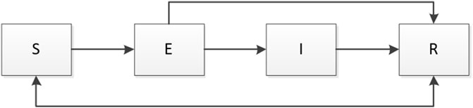
FIGURE 1. Flow chart of the malware propagation model.

Above all, the malware propagation model of fractional order based on the SEIR theory can be represented as Eq. 2.8.

\{\begin{cases} {}_{0}^{C}D_{t}^{α} S (t) = - γ (I + E) S - δ S + R (t - τ_{1}), \\ {}_{0}^{C}D_{t}^{α} E (t) = γ (I + E) S - E (t - τ_{2}) - δ E, \\ {}_{0}^{C}D_{t}^{α} I (t) = E (t - τ_{2}) - η I, \\ {}_{0}^{C}D_{t}^{α} R (t) = δ S + δ E + η I - R (t - τ_{1}) . \end{cases}

(2.8)

The recovered nodes will become susceptible again after the protected period of τ₁, it means that a rate of the recovered nodes become susceptible approximately at any time. After some period of τ₂, the exposed node develops an infected. It also means that a rate of the exposed nodes become infected approximately at any time. To simplify theoretical analysis, we transform the system Eq. 2.8 into a non-delay system, which is the common way in epidemic model analysis. Then, the non-delay model can be rewritten as Eq. 2.9.

\{\begin{cases} {}_{0}^{C}D_{t}^{α} S (t) = - γ (I + E) S - δ S + \frac{1}{τ_{1}} R, \\ {}_{0}^{C}D_{t}^{α} E (t) = γ (I + E) S - \frac{1}{τ_{2}} E - δ E, \\ {}_{0}^{C}D_{t}^{α} I (t) = \frac{1}{τ_{2}} E - η I, \\ {}_{0}^{C}D_{t}^{α} R (t) = δ S + δ E + η I - \frac{1}{τ_{1}} R . \end{cases}

(2.9)

The basic reproductive number is a key parameter to represent the infected numbers in an average infection period. Firstly, note that global stability of a malware-free equilibrium (MFE) was introduced [19]. We can calculate the malware-free equilibrium point $P_{F}^{*} = (S^{*}, E^{*}, I^{*}, R^{*})$ by solving the following equations:

\{\begin{cases} - δ S^{*} + \frac{1}{τ_{1}} R^{*} = 0, \\ S^{*} + R^{*} = 1 . \end{cases}

(2.10)

Then, the malware-free equilibrium point $P_{F}^{*}$ is shown as

\{\begin{cases} S^{*} = \frac{1}{1 + δ τ_{1}}, \\ E^{*} = 0, \\ I^{*} = 0, \\ R^{*} = \frac{δ τ_{1}}{1 + δ τ_{1}} . \end{cases}

(2.11)

The Similar method is used to calculate the endemic equilibrium point (EE) of the above model P_E = (S**, E**, I**, R**), which can be calculated from the following equations.

\{\begin{cases} - γ (I^{* *} + E^{* *}) S^{* *} - δ S^{* *} + 1 / τ_{1} R^{* *} = 0, \\ γ (I^{* *} + E^{* *}) S^{* *} - (1 / τ_{2} + δ) E^{* *} = 0, \\ δ S^{* *} + δ E^{* *} + η I^{* *} - 1 / τ_{1} R^{* *} = 0, \\ S^{* *} + E^{* *} + I^{* *} + R^{* *} = 1 . \end{cases}

(2.12)

So the endemic equilibrium point $P_{E}^{*}$ is shown as

\{\begin{cases} S^{* *} = \frac{η + δ η τ_{2}}{γ + η γ τ_{2}}, \\ E^{* *} = \frac{τ_{2} (- η^{2} + η γ - δ η^{2} τ_{1} - δ η^{2} τ_{2} + η^{2} γ τ_{2} - δ^{2} η^{2} τ_{1} τ_{2})}{γ + η^{2} γ τ_{2}^{2} + η γ τ_{1} + η^{2} γ τ_{1} τ_{2} + δ η^{2} γ τ_{1} τ_{2}^{2} + δ η γ τ_{1} τ_{2}}, \\ I^{* *} = \frac{- η + γ - δ η τ_{2} + η γ τ_{2} - δ^{2} η τ_{1} τ_{2}}{γ + η^{2} γ τ_{2}^{2} + η γ τ_{1} + η^{2} γ τ_{1} τ_{2} + δ η^{2} γ τ_{1} τ_{2}^{2} + δ η γ τ_{1} τ_{2}}, \\ R^{* *} = \frac{τ_{1} δ^{2} η τ_{2} + γ τ_{1} δ η^{2} τ_{2}^{2} - τ_{1} δ η^{2} τ_{2} + γ τ_{1} δ η τ_{2} + τ_{1} δ η + γ τ_{1} η^{2} τ_{2} - τ_{1} η^{2} + γ τ_{1} η}{γ + η^{2} γ τ_{2}^{2} + η γ τ_{1} + η^{2} γ τ_{1} τ_{2} + δ η^{2} γ τ_{1} τ_{2}^{2} + δ η γ τ_{1} τ_{2}} . \end{cases}

(2.13)

According to the next matrices generation method (NGM) [20, 21], which can be used to evaluate the stability of the MFE. The main advantage of the NGM is that it allows ones to ignore any uninfected classes and focus only on the infected classes. There are two infected classes in the proposed model. Let X = (E,I)^T, the model Eq. 2.9 takes the following form:

\frac{\partial X}{\partial t} = F - V,

(2.14)

where $F = (\begin{matrix} γ S (E + I) \\ 0 \end{matrix})$ and $V = (\begin{matrix} \frac{1}{τ_{2}} E + δ E \\ - \frac{1}{τ_{2}} E + η I \end{matrix})$ .

We define f and v as the Jacobian matrices of F and V evaluated at the malware-free equilibrium point P_F:

f = (\frac{\partial F}{\partial X}) |_{P_{F}} = (\begin{matrix} γ S^{*} & γ S^{*} \\ 0 & 0 \end{matrix}) = (\begin{matrix} \frac{γ}{1 + δ τ_{1}} & \frac{γ}{1 + δ τ_{1}} \\ 0 & 0 \end{matrix}),

(2.15)

v = (\frac{\partial V}{\partial X}) |_{P_{F}} = (\begin{matrix} \frac{1}{τ_{2}} + δ & 0 \\ - \frac{1}{τ_{2}} & η \end{matrix}) .

(2.16)

The basic reproductive number R₀ is the largest eigenvalue of the matrix fv⁻¹ given by the Eqs. 2.15, 2.16:

f v^{- 1} = (\begin{matrix} \frac{γ (τ_{2} η + 1)}{η (δ τ_{1} + 1) (δ τ_{2} + 1)} & \frac{γ}{η (δ τ_{1} + 1)} \\ 0 & 0 \end{matrix}) .

(2.17)

Hence, the basic reproductive number corresponding to the DFE is in the following form.

R_{0} = ρ (f v^{- 1}) = \frac{γ (τ_{2} η + 1)}{η (δ τ_{1} + 1) (δ τ_{2} + 1)} .

(2.18)

The Jacobian matrix of proposed model at P_F is shown as follows:

J = (\begin{matrix} - γ (I^{*} + E^{*}) - δ & - γ S^{*} & - γ S^{*} & \frac{1}{τ_{1}} \\ γ (I^{*} + E^{*}) & γ S^{*} - \frac{1}{τ_{2}} - δ & γ S^{*} & 0 \\ 0 & \frac{1}{τ_{2}} & - η & 0 \\ δ & δ & η & - \frac{1}{τ_{1}} \end{matrix}) .

(2.19)

The corresponding characteristic equation is shown as Eq. 2.20.

λ^{4} + A_{3} λ^{3} + A_{2} λ^{2} + A_{1} λ + A_{0} = 0,

(2.20)

where

\{\begin{cases} \begin{aligned} A_{3} & = \frac{τ_{1} + τ_{2} + 2 δ τ_{1} τ_{2} + η τ_{1} τ_{2} - S^{*} γ τ_{1} τ_{2} + E^{*} γ τ_{1} τ_{2} + I^{*} γ τ_{1} τ_{2}}{τ_{1} τ_{2}}, \\ A_{2} & = \frac{δ τ_{1} + δ τ_{2} + η τ_{1} + η τ_{2} + δ^{2} τ_{1} τ_{2} + E^{*} γ τ_{1} + E^{*} γ τ_{2} + I^{*} γ τ_{1} + I^{*} δ γ τ_{1} τ_{2} + I^{*} η γ τ_{1} τ_{2}}{τ_{1} τ_{2}} \\ + \frac{I^{*} γ τ_{2} - S^{*} γ τ_{1} - S^{*} γ τ_{2} + 2 δ η τ_{1} τ_{2} + E^{*} δ γ τ_{1} τ_{2} + E^{*} η γ τ_{1} τ_{2} - S^{*} δ γ τ_{1} τ_{2} - S^{*} η γ τ_{1} τ_{2} + 1}{τ_{1} τ_{2}}, \\ A_{1} & = \frac{η + E^{*} γ + I^{*} γ - S^{*} γ + δ η τ_{1} + δ η τ_{2} + δ^{2} η τ_{1} τ_{2} + E^{*} η γ τ_{1} + E^{*} δ η γ τ_{1} τ_{2}}{τ_{1} τ_{2}} \\ + \frac{E^{*} η γ τ_{2} + I^{*} η γ τ_{1} + I^{*} η γ τ_{2} - S^{*} δ γ τ_{1} - S^{*} η γ τ_{2} + I^{*} δ η γ τ_{1} τ_{2} - S^{*} δ η γ τ_{1} τ_{2}}{τ_{1} τ_{2}}, \\ A_{0} & = - \frac{E^{*} δ γ - E^{*} δ γ + I^{*} δ γ - I^{*} η γ}{τ_{1} τ_{2}} . \end{aligned} \end{cases}

(2.21)

According to the stability theory, the MFE is locally asymptotic stable if R₀ < 1; the EE is locally asymptotic stable if R₀ > 1.

3 Optimal control strategy

In this section, the discrete-time malware propagation model of fractional order is established based on Eq. 2.9. Then, the least square algorithm is used to solve the inverse problem and estimate the unknown parameters in the model. Finally, the adaptive model is proposed to determine the optimal control strategy to reduce the spreading of malware.

In Eq. 2.9, η and δ are the rate of users updating the system on the infected nodes and the other nodes, which are always known parameters, while γ, τ₁, τ₂, α are the unknown parameters. Firstly, estimation of these unknown parameters is investigated though the inverse analysis. Let S [n], E [n], I [n], R [n] represent the number of nodes in each group at time t = hn, n ∈ N*, which is obtained from the designed experiment. Denote h as the constant time step [22].

The discrete-time fractional order Caputo operator Δ^α with numerical approximation is defined in the following form [23–25],

\begin{matrix} Δ^{α} X [n] = \frac{h^{- α}}{Γ (2 - α)} \sum_{j = 0}^{n} (X [n - j + 1] - X [n - j]) ({(j + 1)}^{1 - α} - h^{1 - α}) \\ = \frac{h^{- α}}{Γ (2 - α)} \sum_{j = 0}^{n} b_{n j} . \end{matrix}

(3.1)

Here we denote b_nj = (X [n − j + 1] − X [n − j]) ((j + 1)^1−α − h^1−α). Hence, the recursive function is obtained as Eq. 3.2. The state X [n + 1] can be calculated from state before,

X [n + 1] = (Δ^{α} X [n] - \frac{h^{- α}}{Γ (2 - α)} \sum_{j = 1}^{n} b_{n j}) \frac{Γ (2 - α)}{h^{- α}} + X [n] .

(3.2)

Then, the discrete-time fractional order model is expressed as the following form.

\{\begin{cases} Δ^{α} S [n] = - γ (I [n] + E [n]) S [n] - δ S [n] + \frac{1}{τ_{1}} R [n], \\ Δ^{α} E [n] = γ (I [n] + E [n]) S [n] - \frac{1}{τ_{2}} E [n] - δ E [n], \\ Δ^{α} I [n] = \frac{1}{τ_{2}} E [n] - η I [n], \\ Δ^{α} R [n] = δ S [n] + δ E [n] + η I [n] - \frac{1}{τ_{1}} R [n] . \end{cases}

(3.3)

Begin from initial state (S [0], E [0], I [0], R [0]), the next state $(\hat{S [1]}, \hat{E [1]}, \hat{I [1]}, \hat{R [1]})$ can be calculated though Eqs. 3.2, 3.3. Repeating these process, the state $(\hat{S [n + 1]}, \hat{E [n + 1]}, \hat{I [n + 1]}, \hat{R [n + 1]})$ can be calculated from the state before. The objective of the inverse problem is to minimize the ordinary least squares norm of measured number of nodes in each group and the calculated number of nodes in each group. The objective function is the sum of squared errors between measured number of each group with calculated, which is shown in the following form,

G = \sum_{n} ({(\hat{S [n]} - S [n])}^{2} + {(\hat{E [n]} - E [n])}^{2} + {(\hat{I [n]} - I [n])}^{2} + {(\hat{R [n]} - R [n])}^{2}) .

(3.4)

Then, the parameters γ, τ₁, τ₂, α can be estimated form the solution of the direct problem in the following form,

\hat{γ}, \hat{τ_{1}}, \hat{τ_{2}}, α = a r g m i n G (γ, τ_{1}, τ_{2}, α) .

(3.5)

For estimating the unknown parameters in the propagation model, the gradient descent algorithm [26] is used for minimizing the least squares norm Eq. 3.4.

In above control strategy, the control parameters η and δ are constant in the propagation. In many senses, it may be not the optimal control strategy. The adaptive model is proposed based on the parameters $\hat{γ}, \hat{τ_{1}}, \hat{τ_{2}}, α$ obtained before. Denoted c as the unit cost of update system on one node from attacking in WSNs, which is a constant. When the endemic equilibrium point reached, the total cost at time t = hn can be calculated in the following form,

C = c \times (η_{n} \times I [n] + δ_{n} \times (1 - I [n])),

(3.6)

Algorithm 1. Gradient Descent Algorithm.

1: Input: Starting point V = [γ, τ₁, τ₂, α] ∈ R⁴, a function $\frac{\partial G (V)}{\partial V}$ , step-size β, tolerance θ

2: repeat

3: Calculate $\frac{\partial G (V)}{\partial V}$

4: Update $V = V - β \frac{\partial G (V)}{\partial V}$

5: until ΔX < θ for 100 iterations in sequence

Output: some hopefully minimizing V

where η_n and δ_n are the control parameters at time t = hn.

The control strategy is valid if the number of infected nodes and exposed nodes is larger than the predetermined threshold (Thr). It can be expressed as the given form,

I [n + 1] + E [n + 1] < T h r, n = 1,2, \dots .

(3.7)

The density of exposed nodes and infectious nodes at time t = (n + 1)h can be calculated by the density at time t = nh,

\{\begin{cases} E [n + 1] = (Δ^{α} E [n] - \frac{h^{- α}}{Γ (2 - α)} \sum_{j = 1}^{n} b_{n j}) \frac{Γ (2 - α)}{h^{- α}} + E [n], \\ I [n + 1] = (Δ^{α} I [n] - \frac{h^{- α}}{Γ (2 - α)} \sum_{j = 1}^{n} b_{n j}) \frac{Γ (2 - α)}{h^{- α}} + I [n] . \end{cases}

(3.8)

The control parameters η_n and δ_n are always less than 1 and the η_n ia larger than δ_n at each control stage,

\{\begin{cases} 0 < δ_{n}, η_{n} < 1, \\ η_{n} > δ_{n} . \end{cases}

(3.9)

Based on the above analysis, the optimal control parameters η_n and δ_n can be obtained from the following model,

\begin{aligned} \hat{η_{n}}, \hat{δ_{n}} = a r g m i n c \times (η_{n} \times I [n] + δ_{n} \times (1 - I [n])) \\ s . t . \{\begin{cases} I [n + 1] + E [n + 1] < T h r \\ E [n + 1] = (Δ^{α} E [n] - \frac{h^{- α}}{Γ (2 - α)} \sum_{j = 1}^{n} b_{n j}) \frac{Γ (2 - α)}{h^{- α}} + E [n], \\ I [n + 1] = (Δ^{α} I [n] - \frac{h^{- α}}{Γ (2 - α)} \sum_{j = 1}^{n} b_{n j}) \frac{Γ (2 - α)}{h^{- α}} + I [n], \\ 0 < δ_{n}, η_{n} < 1, \\ η_{n} > δ_{n} . \end{cases} \end{aligned}

(3.10)

By solving the nonlinear model, we can get the optimal strategy of the rate of the update system.

4 Simulations and results

To evaluate the performance of the proposed models, we carry out the experiments to obtain the data of malware propagation over a period of 730 unit time. At the beginning of the experiment, there are 1,000 sensor nodes lying in the WSN. The unknown malicious programme spread in this WSNs in this period. We set the initial control parameters η = 0.02 and δ = 0.0003. There are 10,000 nodes in this WSN and the initial state of the WSNs is S (0) = 0.9, E (0) = 0.1, I (0) = R (0) = 0. According to the obtained experiment data, the number of susceptible nodes will decrease within the time. The number of exposed nodes will increase at the beginning of the experiment and then decrease radially, the number will keep stable at the end of the experiment. The number of infected nodes and recovered nodes will increase within the time.

By using gradient descent algorithm to estimate the parameters γ, τ₁, τ₂, α by solving Eq. 3.5 with MATLAB. The results are obtained γ = 0.000023, τ₁ = 56.21,τ₂ = 6.10, α = 0.65. We also tried to fit the integer order model (α = 1) to the experiment data. The results can be obtained as γ = 0.000112, τ₁ = 25.31, τ₂ = 11.18.

Based on the estimated parameters, the behavior of propagation in each group based on the fractional order and integer order are shown in Figures 2–5.

FIGURE 2

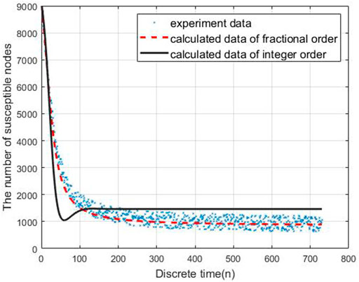
FIGURE 2. Model results for suspected nodes.

FIGURE 3

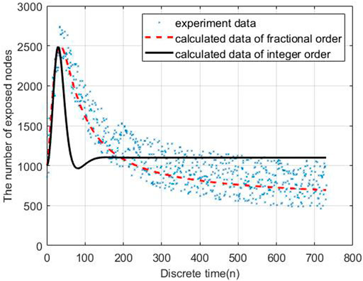
FIGURE 3. Model results for exposed nodes.

FIGURE 4

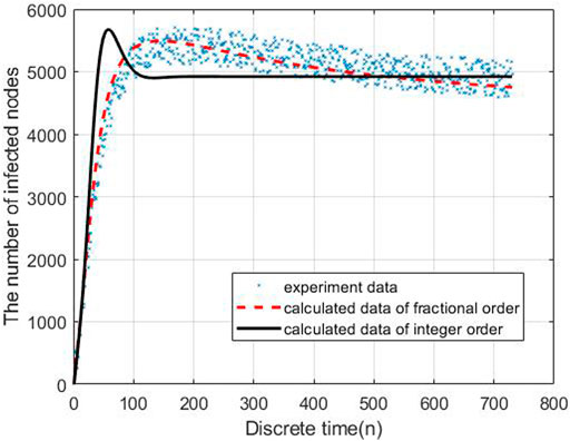
FIGURE 4. Model results for infected nodes.

FIGURE 5

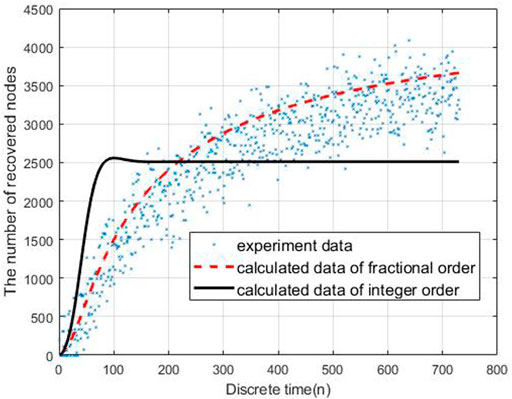
FIGURE 5. Model results for recovered nodes.

As Figures 2–5 shown, the fractional order model works better than the propagation model of integer order. Especially, the behavior of recovered nodes propagation in fractional order is more accuracy than that in integer order.

Based on the parameters estimated above, the reproductive number of this malware propagation can be calculated R₀ = 0.0137, R₀ < 1. However, the number of infected nodes and exposed is so large, it means the control parameters need to be improved. The optimal control model is established to estimate the parameter η_n, δ_n at time t = nh according to Eq. 3.10 if the number of infected nodes and exposed is less than 10%.

By solving Eq. 3.7, the performance of the optimal control strategy is shown in Figures 6–9.

FIGURE 6

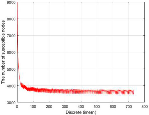
FIGURE 6. Simulation of the free suspected nodes.

FIGURE 7

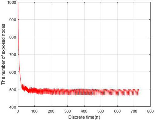
FIGURE 7. Simulation of the infectious nodes.

FIGURE 8

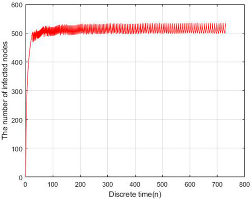
FIGURE 8. Simulation of the free exposed nodes.

FIGURE 9

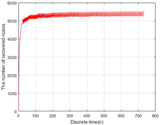
FIGURE 9. Simulation of the infectious nodes.

The adaptive control parameters at each time is shown in Figures 10, 11.

FIGURE 10

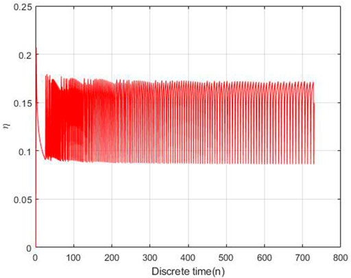
FIGURE 10. The control parameter η at each time.

FIGURE 11

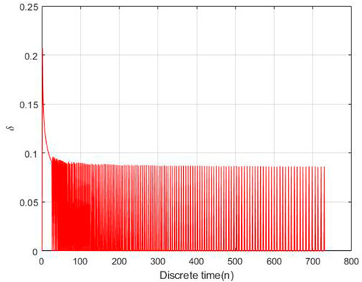
FIGURE 11. The control parameter δ at each time.

As Figures 10, 11 shown, the control parameters are oscillation to keeping the number of exposed nodes and infection nodes is less than 10% of the total number. The parameters η is larger than δ, while η is oscillation between 0.18 and 0.095, δ is oscillation between 0.095 and 0. This is the optimal control strategy by solving Eq. 3.10 based on the gradient descent algorithm.

5 Conclusion

In recent years, differential equations of fractional order have been increasingly used to describe problems in optical systems, rheology, mechanical systems, signal processing and other application fields. However, unlike the classical integer order derivatives, there exists a number of different definitions of fractional order derivatives and corresponding equations. These definition differences lead to differential equations of fractional order having similar form but significantly different properties. It also means that given a differential equations of fractional order, there exists no well-defined method to analyze them systematically. Therefore, it is an urgent task to establish and improve the SEIR epidemic theory of fractional order.

The malware propagation model of fractional order is established based on the classical SEIR epidemic theory, and the stability condition of the model is also analyzed in this paper. The inverse approach for the uncertainty propagation is discussed to estimate the unknown parameters in the model by using the discrete element method and least square algorithm. Finally, the adaptive control strategy is proposed to minimizing the number of the infected nodes and exposed nodes in the WSN at any time. Simulation results show the fractional order model works better than the propagation model of integer order and the adaptive control strategy is better than the fixed control strategy.

There are also some limitations of our work. It must be pointed out here that the solutions of the time fractional differential equations are not very smooth in the temporal directions [23–25]. That means we need to use the L1-scheme on the graded meshes in order to improve the convergent results. In our work, many engineering aspects such as protocol, communication bit rate, noise, delay are not considered. However, we have certain difficulties in this area of knowledge, which is also the work we need to consider in the future.

Data availability statement

The raw data supporting the conclusions of this article will be made available by the authors, without undue reservation.

Author contributions

All authors listed have made a substantial, direct, and intellectual contribution to the work and approved it for publication.

Conflict of interest

The authors declare that the research was conducted in the absence of any commercial or financial relationships that could be construed as a potential conflict of interest.

Publisher’s note

All claims expressed in this article are solely those of the authors and do not necessarily represent those of their affiliated organizations, or those of the publisher, the editors and the reviewers. Any product that may be evaluated in this article, or claim that may be made by its manufacturer, is not guaranteed or endorsed by the publisher.

References

1. Yousefpoor MS, Yousefpoor E, Barati H, Barati A, Movaghar A, Hosseinzadeh M. Secure data aggregation methods and countermeasures against various attacks in wireless sensor networks: A comprehensive review. J Netw Comp Appl (2021) 190:103118. doi:10.1016/j.jnca.2021.103118

CrossRef Full Text | Google Scholar

2. Zhu L, Zhao HY, Wang X. Bifurcation analysis of a delay reaction-diffusion malware propagation model with feedback control. Commun Nonlinear Sci Numer Simul (2015) 22:747–68. doi:10.1016/j.cnsns.2014.08.027

CrossRef Full Text | Google Scholar

3. Nwokoye C, Umeh I. Analytic-agent cyber dynamical systems analysis and design method for modeling spatio-temporal factors of malware propagation in wireless sensor networks. MethodsX (2018) 5:1373–98. doi:10.1016/j.mex.2018.10.005

PubMed Abstract | CrossRef Full Text | Google Scholar

4. Bandirmali N, Erturk I. WSNSec: A scalable data link layer security protocol for WSNs. Ad Hoc Networks (2012) 10(1):37–45. doi:10.1016/j.adhoc.2011.04.013

CrossRef Full Text | Google Scholar

5. Chandnani N, Khairnar CN. An analysis of architecture, framework, security and challenging aspects for data aggregation and routing techniques in IoT WSNs. Theor Comp Sci (2022) 929:95–113. doi:10.1016/j.tcs.2022.06.032

CrossRef Full Text | Google Scholar

6. Shen S, Zhou H, Feng S, Huang L, Liu J, Yu S, et al. Hsird: A model for characterizing dynamics of malware diffusion in heterogeneous WSNs. J Netw Comp Appl (2019) 146:102420. doi:10.1016/j.jnca.2019.102420

CrossRef Full Text | Google Scholar

7. Srivastava PK, Pandey SP, Gupta N, Singh SP, Ojha RP. Modeling and analysis of antimalware effect on wireless sensor network. In: 2019 IEEE 4th International Conference on Computer and Communication Systems (ICCCS); February 23-25, 2019; Singapore (2019). p. 639–43.

CrossRef Full Text | Google Scholar

8. Zhou H, Shen S, Liu J. Malware propagation model in wireless sensor networks under attack–defense confrontation. Comp Commun (2020) 162:51–8. doi:10.1016/j.comcom.2020.08.009

CrossRef Full Text | Google Scholar

9. Zhu L, Zhao H. Dynamical analysis and optimal control for a malware propagation model in an information network. Neurocomputing (2015) 149:1370–86. doi:10.1016/j.neucom.2014.08.060

CrossRef Full Text | Google Scholar

10. Hosseini S, Ma A. The dynamics of an SEIRS-QV malware propagation model in heterogeneous networks. Physica A (2018) 512:803–17. doi:10.1016/j.physa.2018.08.081

CrossRef Full Text | Google Scholar

11. Guillen JDH, Rey AMD. A mathematical model for malware spread on WSNs with population dynamics. Physica A (2020) 545:123609. doi:10.1016/j.physa.2019.123609

CrossRef Full Text | Google Scholar

12. Kumari S, Upadhyay RK. Exploring the behavior of malware propagation on mobile wireless sensor networks: Stability and control analysis. Mathematics Comput Simulation (2021) 190:246–69. doi:10.1016/j.matcom.2021.05.027

CrossRef Full Text | Google Scholar

13. Ahmed E, Elgazzar AS. On fractional order differential equations model for nonlocal epidemics. Physica A (2007) 379:607–14. doi:10.1016/j.physa.2007.01.010

PubMed Abstract | CrossRef Full Text | Google Scholar

14. Momani S, Kumar R, Srivastava HM, Kumar S, Hadid S. A chaos study of fractional SIR epidemic model of childhood diseases. Results Phys (2021) 27:104422. doi:10.1016/j.rinp.2021.104422

CrossRef Full Text | Google Scholar

15. Coll C, Herrero A, Ginestar D, Sanchez E. The discrete fractional order difference applied to an epidemic model with indirect transmission. Appl Math Model (2022) 103:636–48. doi:10.1016/j.apm.2021.11.002

CrossRef Full Text | Google Scholar

16. Abbes A, Ouannas A, Shawagfeh N, Grassi G. The effect of the Caputo fractional difference operator on a new discrete COVID-19 model. Results Phys (2022) 39:105797. doi:10.1016/j.rinp.2022.105797

PubMed Abstract | CrossRef Full Text | Google Scholar

17. Zhu Z, Lu J. Robust stability and stabilization of hybrid fractional-order multi-dimensional systems with interval uncertainties: An LMI approach. Appl Math Comput (2021) 401:126075. doi:10.1016/j.amc.2021.126075

CrossRef Full Text | Google Scholar

18. Arenas AJ, Gonzalez-Parra G, Chen-Charpentier BM. Construction of nonstandard finite difference schemes for the SI and SIR epidemic models of fractional order. Math Comput Simulation (2016) 121:48–63. doi:10.1016/j.matcom.2015.09.001

CrossRef Full Text | Google Scholar

19. Verma T, Gupta AK. Network synchronization, stability and rhythmic processes in a diffusive mean-field coupled SEIR model. Commun Nonlinear Sci Numer Simul (2021) 102:105927. doi:10.1016/j.cnsns.2021.105927

PubMed Abstract | CrossRef Full Text | Google Scholar

20. Abdulwasaa MA, Abdo MS, Shah K, Nofal TA, Abdel-Aty AH, Kawale SV, et al. Fractal-fractional mathematical modeling and forecasting of new cases and deaths of COVID-19 epidemic outbreaks in India. Results Phys (2021) 20:103702. doi:10.1016/j.rinp.2020.103702

PubMed Abstract | CrossRef Full Text | Google Scholar

21. Wei F, Xue R. Stability and extinction of SEIR epidemic models with generalized nonlinear incidence. Math Comput Simulation (2020) 170:1–15. doi:10.1016/j.matcom.2018.09.029

CrossRef Full Text | Google Scholar

22. Sene N. Introduction to the fractional-order chaotic system under fractional operator in Caputo sense. Alexandria Eng J (2021) 60:3997–4014. doi:10.1016/j.aej.2021.02.056

CrossRef Full Text | Google Scholar

23. Yan YB, Khan M, Ford NJ. An analysis of the modified L1 scheme for time-fractional partial differential equations with nonsmooth data. Siam J Numer Anal (2018) 56(1):210–27. doi:10.1137/16m1094257

CrossRef Full Text | Google Scholar

24. Li D, Wu C, Zhang Z. Linearized galerkin FEMs for nonlinear time fractional parabolic problems with non-smooth solutions in time direction. J Scientific Comput (2019) 80(1):403–19. doi:10.1007/s10915-019-00943-0

CrossRef Full Text | Google Scholar

25. Zhou B, Chen X, Li D. Nonuniform alikhanov linearized galerkin finite element methods for nonlinear time-fractional parabolic equations. J Scientific Comput (2020) 85(2):39. doi:10.1007/s10915-020-01350-6

CrossRef Full Text | Google Scholar

26. Khan S, Ahmad J, Naseem I, Moinuddin M. A novel fractional gradient-based learning algorithm for recurrent neural networks. Circuits Syst Signal Process (2018) 37:593–612. doi:10.1007/s00034-017-0572-z

CrossRef Full Text | Google Scholar

Keywords: malware propagation, fractional order difference equations, inverse approach, discrete element method, adaptive model

Citation: Zhou Y, Liu B-T, Zhou K and Shen S-F (2023) Malware propagation model of fractional order, optimal control strategy and simulations. Front. Phys. 11:1201053. doi: 10.3389/fphy.2023.1201053

Received: 06 April 2023; Accepted: 23 May 2023;
Published: 08 June 2023.

Edited by:

Zhouchao Wei, China University of Geosciences Wuhan, China

Reviewed by:

Dongfang Li, Huazhong University of Science and Technology, China
Jesus Manuel Munoz-Pacheco, Benemérita Universidad Autónoma de Puebla, Mexico

Copyright © 2023 Zhou, Liu, Zhou and Shen. This is an open-access article distributed under the terms of the Creative Commons Attribution License (CC BY). The use, distribution or reproduction in other forums is permitted, provided the original author(s) and the copyright owner(s) are credited and that the original publication in this journal is cited, in accordance with accepted academic practice. No use, distribution or reproduction is permitted which does not comply with these terms.

*Correspondence: Shou-Feng Shen, mathssf@zjut.edu.cn

ORIGINAL RESEARCH article

Malware propagation model of fractional order, optimal control strategy and simulations

1 Introduction

2 Malware propagation model of fractional order

3 Optimal control strategy

4 Simulations and results

5 Conclusion

Data availability statement

Author contributions

Conflict of interest

Publisher’s note

References

This article is part of the Research Topic

People also looked at