 Bjarn Van Riet
 Simon Six3
 Kristine Walraevens
 Thomas Hermans
- 1Laboratory for Applied Geology and Hydrogeology, Department of Geology, Ghent University, Ghent, Belgium
- 2Antea Group, Antwerp, Belgium
- 3De Watergroep, Brussels, Belgium
Fractured and karst aquifers are important groundwater reservoirs and are widely used to provide drinking water to the population. Because of the presence of the fractures with varying geometry and properties providing preferential flow paths, fractured aquifers are highly heterogeneous and difficult to characterize and model. In this context, geophysical methods can provide relevant spatially distributed data about the presence of fractures, that can be further integrated in hydrological and groundwater models. In this contribution, we present a case study of a groundwater extraction site in a fractured chalk aquifer in Voort (Belgium), used for the production of drinking water. First, the presence of fractures in the vicinity of the extraction site and their orientation is imaged using electrical resistivity tomography. Based on the available data and the objectives of the study, it is chosen to model only the groundwater component and to simplify the unsaturated zone processes through an average recharge rate. Then, the detected fractures are included in the groundwater model to improve the calibration and the predictive capacity of the model. The results show that a set of parallel fractures crosses the modeled area, whose orientation is in accordance with the tectonic setting. Including these fractures in the model, a more satisfactory calibration was achieved, helping to better understand the hydrogeological behavior of the aquifer. Finally, the acquired knowledge is used to propose new management scenarios for the extraction site minimizing its impact.
Introduction
Fractured and karst aquifers are important groundwater reservoirs and are worldwide used to provide drinking water to the population. In contrast to unconsolidated sedimentary aquifers, in which flow can generally be considered as relatively uniform, fractured aquifers are highly heterogeneous. The fractures provide preferential pathways for fluid flow in originally low permeable rocks (Nelson, 1985). These structural weaknesses have been proven important for recharge processes, reservoir and seal behavior and typically increase the maximum achievable flow rate in water extractions (e.g., Travis, 1984; Bear, 1993).
The characterization of fractured aquifers remains particularly complicated. In recent years, many efforts have been made to characterize fractures (e.g., Guevara-Mansilla et al., 2020; Molron et al., 2020; Mézquita González et al., 2021), to model them using discrete fracture network (Maillot et al., 2016; Medici et al., 2021) or to include those characteristics in calibration processes (Ringel et al., 2019; Medici et al., 2021). However, the identification of individual fractures can only be made locally using borehole data or high-resolution geophysical methods such as ground penetrating radar (Molron et al., 2020). For water management purposes, it is generally illusory to include every single fractures in a conceptual or numerical model of the aquifer. What is relevant is the effect of the fractures at the catchment scale. If the distribution of the fractures is relatively homogeneous, the aquifer can be modeled using equivalent porous media properties (Berkowitz, 2002; Lemieux et al., 2006; Medici et al., 2019, 2021). Nevertheless, in many instances, the geometry, aperture and density of fractures is varying spatially, resulting in a heterogeneous distribution of the hydraulic properties at the scale of a catchment or water extraction site (Wang et al., 2016; Masciopinto et al., 2017). However, because of the lack of accurate information, fracture zones are rarely explicitly included in modeling efforts, except when they are clearly identified, for example along major faults (Hill et al., 2010; Gallegos et al., 2013; Saller et al., 2013).
In this context, geophysical methods can bring relevant information to characterize the structure of the aquifer and reveal the presence of fractured zones (e.g., Robert et al., 2011; Binley et al., 2015; Van Hoorde et al., 2017). Given their sensitivity to the porosity and water content, electromagnetic methods are particularly suited for the characterization of fractures inducing a secondary porosity (Schmutz et al., 2011; Mézquita González et al., 2021). Recently, airborne electromagnetic surveys have gained popularity as they can provide dense information at the catchment-scale up to a depth of several hundred meters (e.g., Barfod et al., 2018; Knight et al., 2018; Vilhelmsen et al., 2018; Minsley et al., 2021). However, airborne surveys require relatively high investment costs that are difficult to support for small drinking water companies without external (governmental) support. In addition, such surveys are often difficult in densely populated areas (urban and peri-urban areas) and may lack the required resolution to detect small-scale fracture zones. In such a case, electrical resistivity tomography (ERT) provides a useful alternatives (e.g., Cheng et al., 2019; Cong-Thi et al., 2021; Zarate et al., 2021). Although ERT is more time consuming than airborne surveys and does not allow as dense data coverage, it is a robust method that can provide reliable information at the catchment scale (Miller et al., 2008).
In this paper, we present the case study of a water extraction site in Voort, in the south of the province of Limburg, Belgium (Figure 1A). It is situated in a semi-confined fractured chalk aquifer. In this aquifer, the distribution of drawdown around the pumping wells shows some unexpected anomalies that are thought to be the results of the presence of preferential flow paths along fractures located in topographical depressions. In a first step, we investigate the extent of the fractured area using ERT. A series of ERT profiles is used to identify the location of the main fractures and their orientation. Based on this first assessment and the objectives of the study, it was chosen to simplify the processes taking place in the unsaturated through an average and constant recharge rate and to focus on the groundwater component. Then, the fractured zones are implemented into the groundwater model using Modflow (Harbaugh, 2005). We discuss the benefits and limitations of explicitly including the identified fracture zones in the model in comparison to a homogenous equivalent porous medium model approach. Finally, the model is used to simulate future extraction scenarios and resulting drawdowns, including an increased pumping rate and the installation of a new pumping well within and outside a fractured zone.
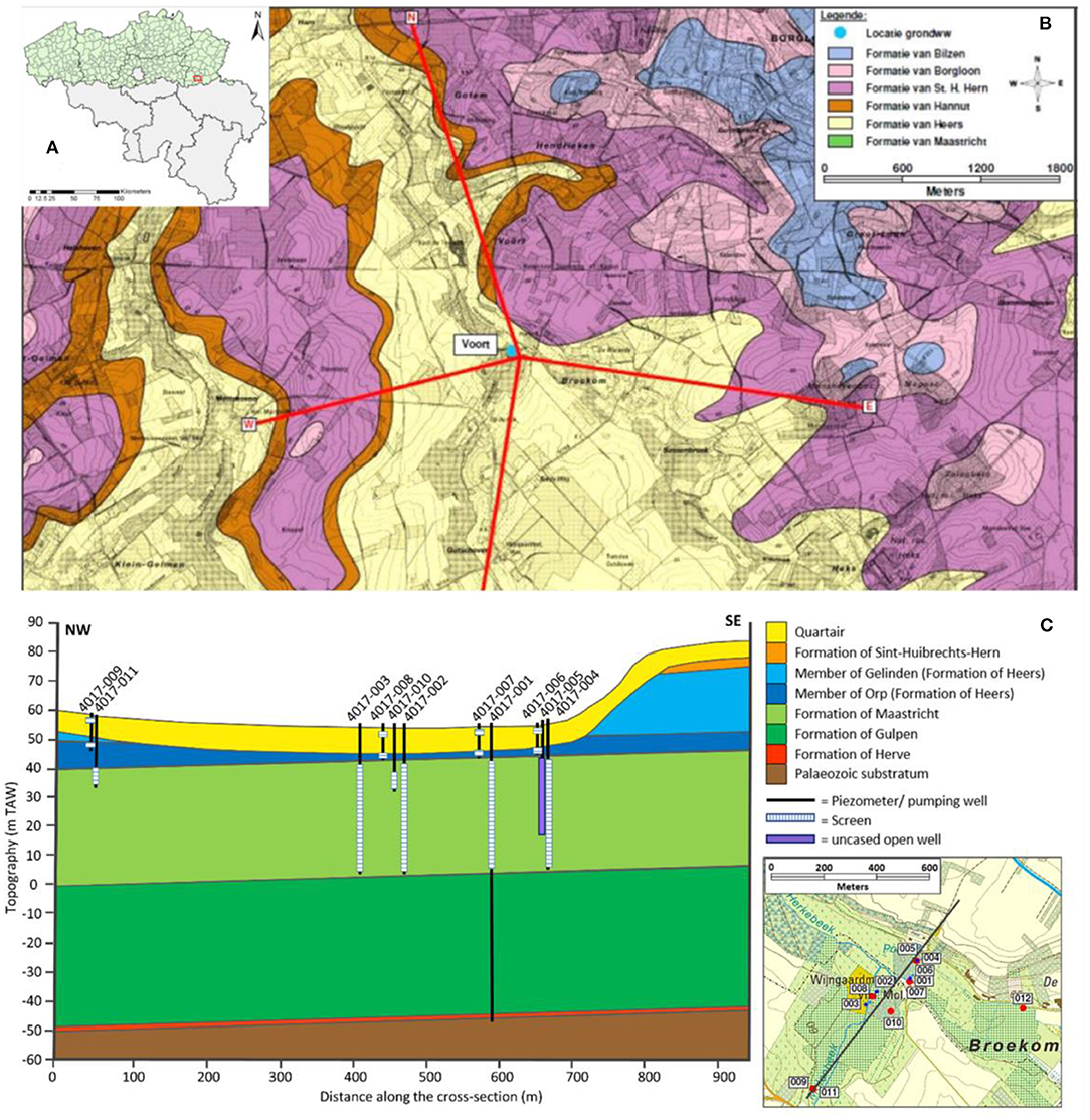
Figure 1. (A) Map of Belgium and indication the extraction site (red). (B) Geological map of the study area. (C) Plan map and cross-section through the center of the extraction site.
Geology and Hydrogeology of the Study Site
The study site is located in Voort, Limburg (Belgium) in the Cretaceous aquifer system which lies on top of the Palaeozoic substratum (Figure 1). The Cretaceous aquifer system consists of three geological formations (Claes and Willems, 1997). At the basis, the Formation of Herve consists mostly of poorly permeable smectite (Thorez and Monjoie, 1973) and is considered as the bottom aquitard (impermeable boundary) for the groundwater model. Above the smectite, the compacted grey chalk from the Formation of Gulpen, about 47 m thick at the extraction site has a relatively low permeability. The aquifer itself is constituted by the more permeable fine to coarse yellowish chalk of the Formation of Maastricht. The latter is 38 m thick and contains some layers abundant in flint (Van Den Eeckhaut et al., 2007). Furthermore, although the Cretaceous chalk can be considered relatively homogeneous (Vandersteen et al., 2014), its top is fractured, which locally increases its permeability.
Above the Cretaceous system lies the Palaeocene aquifer system, consisting in an alternance of clay, silt and sandy layers. It contains the Formations of Heers and Hannut. At the basis of the former formation, the Member of Orp mainly consists of clay with some fine glauconiferous marine sands (Deckers et al., 2014). This layer is poorly permeable and serves as a seal for the underlying fractured aquifer. In the valleys the member is however on average only 8 m thick. This causes the Cretaceous aquifer to be only semi-confined. Above this semi-confining layer, the Member of Gelinden consists of whitish, crumbly, marly chalk (Vandenberghe et al., 2004; De Bast et al., 2013) and is relatively permeable. It serves as a secondary aquifer. The member is up to 25 m thick in crests but is absent in the deeper valleys of the study area. Seepage from this member has been observed (De Watergroep, 2014). The Formation of Hannut consists of poorly permeable clay and silt covered by glauconitic fine sands (De Geyter, 1988; Laga et al., 2001; Yans et al., 2005) and only occurs in the high elevation parts of the study area. Locally on the crests, the Formation of Boom, consisting of firm clay, is found (Claes and Willems, 1997). On top of the Palaeocene aquifer system, the Oligocene aquifer system is present in the crests. This aquifer system contains the Formations of Sint-Huibrechts-Hern, Borgloon, and Bilzen with a succession of permeable and confining layers made of clay, silt and sands (Laga, 1988; Cadée, 1991; Maréchal, 1993; Claes and Willems, 1997; Van Den Eeckhaut et al., 2007).
Finally, the entire study area is covered with Quaternary sediments with an average thickness of 10 m (De Watergroep, 2014). The thickness increases toward the valleys and gets very thin on steep hill slopes. The sediments consist of loam, peat and an admixture of gravel (De Watergroep, 2014). It has an overall mediocre permeability, but this can greatly vary due to local differences in its structure and composition (De Watergroep, 2014).
In Voort, the drinking water company De Watergroep has a permit to extract 2,190,000 m3/year from the chalk aquifer. Four pumping wells were drilled in the center of a small valley and screened over the whole thickness of the Maastricht formation. In addition, a series of monitoring piezometers were drilled to monitor the drawdown resulting from the extraction activities. These piezometers are distributed in the Formation of Maastricht, but also in the superficial layers. For logistical reasons, De Watergroep wants to close some small extraction sites in the vicinity and increase the extraction rate at Voort. However, the evolution of the hydraulic head in the monitored piezometers show a possible influence of fractured zones in the distribution of the drawdown. A hydrological model is thus needed to assess if the increase of the extraction rate is possible without excessive increase of the drawdown, including in the overlying layers.
Geophysical Measurements
Principles and Setup
To study the location, density and the pattern of fractures in the top of the Cretaceous, an ERT survey was conducted. ERT is used to determine the electrical resistivity of geological layers, by achieving 2D or 3D inverted sections (Loke et al., 2013). ERT is suitable for many hydrogeological applications (Binley et al., 2015) such as locating cavities and fractures or estimating layer thicknesses and detecting interfaces between layers (e.g., Guérin, 2005; Al-Tarazi et al., 2006; Guérin et al., 2009; Robert et al., 2011; Van Hoorde et al., 2017). It has also been used together with tracer experiments to identify preferential flow paths and solute transport processes along fractures (e.g., Robert et al., 2012) or image infiltrating processes in the unsaturated zone (Lesparre et al., 2017; Claes et al., 2019; Blazevic et al., 2020).
In this study, we assume that the fractures are creating a secondary porosity in the rock matrix, therefore increasing the water content in the saturated zone. The resistivity of the chalk is much higher than that of water (e.g., Reninger et al., 2014; Katika et al., 2018). In fractured zones, more water is present. According to petrophysical laws (Revil et al., 2017), this is accompanied by a decrease in electrical resistivity. We also expect a contrast in resistivity between the consolidated chalk deposits and the overlying unconsolidated clastic (sand, silt, and clay) sediments.
A total of six profiles were arranged in the studied catchment with different lengths and in different directions traversing both the valleys and the hillsides (Figure 2) to accurately image the local pattern of fractures. The first four profiles were initially laid out to verify if fractured zones were limited to the valleys as originally assumed. Profiles 5 and 6 were later collected to assess the continuity and orientation of the previously identified fracture zones. Four profiles (profiles 1, 3, 5, and 6) were set out around the four pumping wells in the center of the study area, while profiles 2 and 4 are located further away on hill slope and crests.
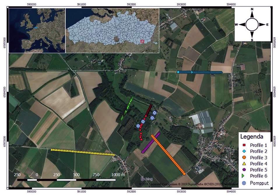
Figure 2. Location of the ERT profiles.
The ERT data were collected using an ABEM terrameter LS with 5 m electrode spacing. A multi-gradient electrode configuration was adopted (Dahlin and Zhou, 2006), given its relatively good resolution to detect lateral variations and its high signal-to-noise ratio. Each initial profile comprised 64 electrodes and 1,392 measured resistances. However, when possible, the profiles were extended using the roll-along technique.
Noise Characterization
It is crucial to accurately quantify the noise to prevent misinterpretation of ERT images (LaBrecque et al., 1996). Overestimation of the noise can lead to gross smoothing of structures, while an underestimation of noise can create artificial structures (Slater et al., 2000). Noise can arise from several factors like poor electrode contact, random errors attributed to the measurement device and errors arising from external factors (background noise) (Slater et al., 2000). To estimate the error on the ERT measurements, reciprocal measurements were collected for a subset of the data set. Overall, an increase of the reciprocal error with raising resistance was observed. Profiles located in the valley showed a very low relative reciprocal error, lower than 1%, while the profiles on the hill slopes and crests showed larger reciprocal errors in the range of 2–4%. For the latter, the substrate was hard after a dry period, increasing the electrode contact resistance, what likely explains the larger reciprocal error. Overall, the quality of measurements is sufficient and can be used for the qualitative interpretation of fractured areas. The error levels are also consistent (within the same range) with the final error of the inversion process (see below).
Data Inversion
The data processing and inversion was accomplished with the software Res2dinv (e.g., Loke, 2006). We used a blocky model constraint (L1 norm) as the expected resistivity distribution resulting from fractures is expected to yield sharp contrasts in resistivity, with lower resistivities concentrated in fracture zones. A L1 norm is also used on the data to minimize the effect of outliers. Before inversion, the apparent resistivity pseudo-section was plotted to remove obvious outliers. After a first inversion, data points with a root-mean-square error larger than 100% were also removed from the data set, to avoid potential artifacts of inversion.
The sensitivity was used to assess the quality of the inversion. An example is given for profile 1 in Figure 3. It shows the classical decrease of sensitivity with depth and on the side of the section, as well as a lower sensitivity in resistive blocks as electrical current flows preferentially in conductive zones. Additionally, in order to check the quality of the obtained images and to derive to which depth the ERT results are reliable, we determine the depth of investigation index (DOI) using two inversion with reference model equal to 0.1 and 10 times the average apparent resistivity, as suggested by Oldenburg and Li (1999). The calculated DOI index is a value between 0 and 1. Indexes approaching zero mean that both inversions produce the same resistivity value. DOI indexes close to one are in contrast not sensitive to surface data anymore but depend mostly on the reference model. We use a threshold of 0.1 for the interpretation of the resistivity images (e.g., Caterina et al., 2013). An example of the DOI is shown for profile 1 (Figure 3C). It shows that the whole section has DOI values lower than 0.1, except for a zone at the border of the section, meaning that we can interpret the variations of resistivity with confidence down to depth around 80 m. Slightly larger DOI are observed in some resistive blocks and at the interface between the chalk aquifer and the overlaying unconsolidated deposits, but they do not prevent the interpretation of the corresponding interfaces.

Figure 3. Profile 1 (A) with sensitivity section (B) and DOI (C).
Results and Interpretation
Several layers can be identified on the ERT profiles (Figures 4A–F). The interpreted top of the Cretaceous is marked as a white dashed line at the location of the contrast between the resistive chalk and the more conductive overburden. In profiles 2, 3, and 4, the layer above is identified as the Formation of Heers. It has a lower conductivity due to a high clay content in the Member of Orp and the high water content in the relatively well-permeable crumbly marl of the Member of Gelinden (Vandenberghe et al., 2004; De Bast et al., 2013; Deckers et al., 2014). The top of this formation is indicated with a white dotted line. The upper layer is interpreted as the Quaternary. These sediments generally have a higher resistivity than the Formation of Heers but the contrast can be very low which complicates separating them like in profiles 1, 5, and 6. ERT is thus able to roughly identify the different geological layers in the upper part of the model. Those layers are laterally relatively homogeneous, so that that the recharge pattern can be expected to be mostly dominated by the topography of the area and the soil occupation and not by preferential infiltration path.
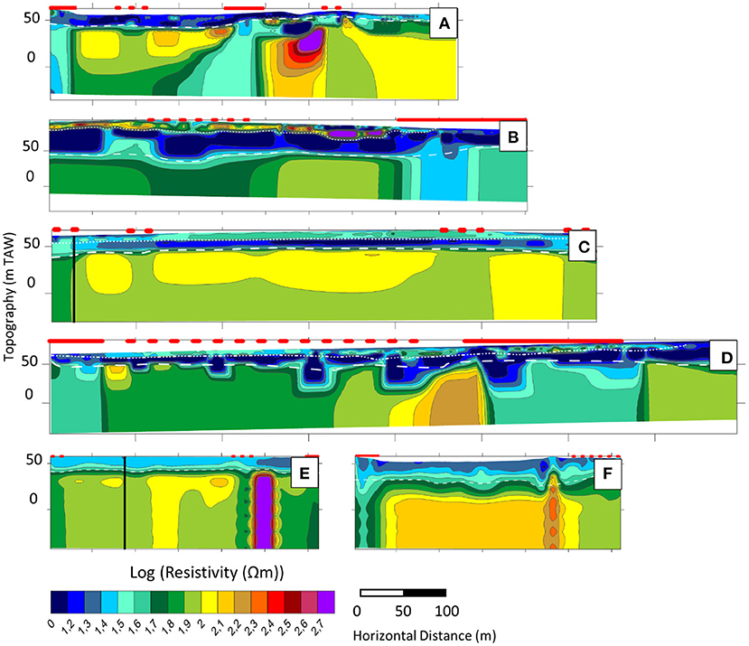
Figure 4. Inversion results with fracture interpretation of profile 1 to 6 (A–F). The full red line shows interpreted fractured zone, dotted red line indicate possible fracture zones. The white dash line indicates the top of the Cretaceous chalk layer and the full white line the bottom of the Quaternary deposits.
Interpreted fractured zones are indicated as full red lines above the profile and correspond to lateral decreases of resistivity in the chalk formations. Smaller contrasts in resistivity are indicated with a dashed red line above the profile, and could correspond to fracture zones with a smaller fracture density or water content. It can be concluded that fractured zones in the top of the Cretaceous are not only found in the valleys (profiles 1, 3, 5, and 6) but also in the hillier parts of the study area (profiles 2 and 4). A second important observation is that profile 3, although located in the valley, does not contain clear fractured regions in the chalk, but only slight contrasts in resistivity. A final important observation is that the fractured zones in profile 1, 5, and 6, seem narrower than the ones in profiles 2 and 4. These observations seem to suggest that the identified fractured zones are subparallel to profile 3 and almost perpendicular to profiles 1, 5 and 6, while they intersect profiles 2 and 4 with an angle.
Most of the available boreholes are limited to the center of the study zone (Figures 1, 2) and it was not possible to systematically measure the profiles in the vicinity of the boreholes. In addition, the chalk aquifer is not outcropping in the study area. For these reasons, it is impossible to validate the identified fractures with ground-truth data. Nevertheless, ERT results are coherent with the expected distribution of geological formations, and the DOI and sensitivity indicate that the identified low resistivity zones in the chalk are in the resolved part of the tomograms. We are thus confident these anomalies correspond to fractured zones and/or zones with preferential dissolution in the chalk. The fracture zones do not seem to generate heterogeneities within the upper part of the model. Only one well is co-located with profile 1 (distance of 275 m along the profile, see Figure 2). No specific indication of fractures was found during drilling, but the well seems rather located in an area where the top of the chalk is globally less resistive, maybe indicating more alteration and dissolution in the top of the chalk aquifer. For tapping in the higher hydraulic conductivity zone, the well should have been placed 50 to 100 m further to the North East.
To better grasp the spatial distribution of the fractures, they are set out on a map in Figure 5. Despite the relatively large uncertainty related to the distance between the parallel profiles, it is possible to propose a tentative connection between some of the fractured zones using the profiles in the center of the study area. The fractures are interpreted to be almost parallel to profile 3, oriented along the northwest-southeast direction. This orientation is also parallel to the relatively nearby Roer Graben (Deckers et al., 2018) and its numerous faults in the western part of Germany, southern part of the Netherlands and eastern part of Belgium. This orientation has been previously identified as the main orientation of fractures (Figure 5B) in the Cretaceous formations (DOV, 2019). The extension of the fracture zones beyond the area investigated by ERT is unknown, but the global analysis of main fractures in the Cretaceous formations tend to show that fractured zones crossing the whole study area can be expected. This assumption will be further investigated with the numerical models.
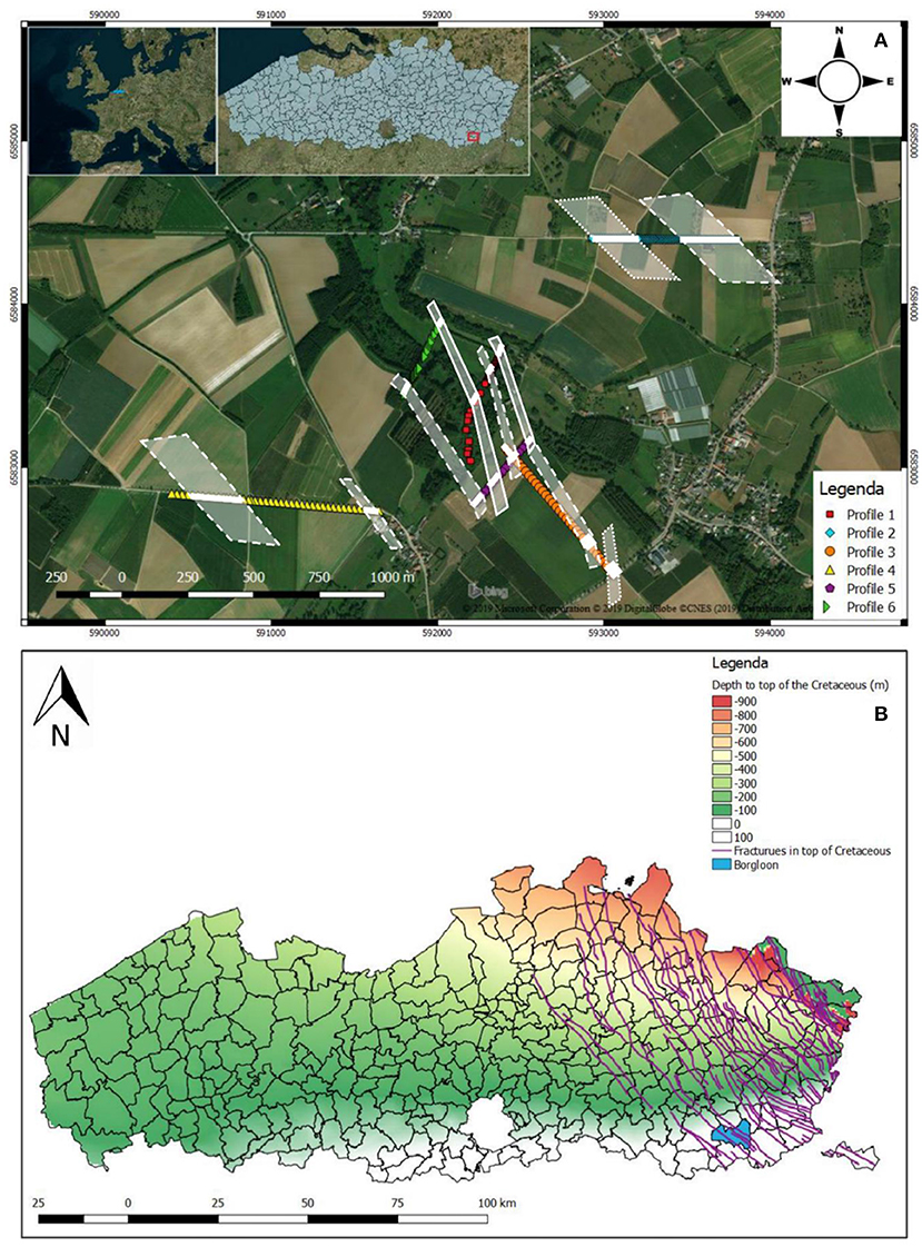
Figure 5. (A) Surface map with indication of identified fractured zones on the six ERT profiles and indication of the possibly linked fractured zones (white dotted line). The full lines are more certain, the dashed lines are less certain, and the dotted lines are the least certain. (B) Fractures in the top Of the Cretaceous in Flanders (purple). The colorscale indicates the depth to the top of the Cretaceous. The municipality of the extraction site is indicated in Blue.
Groundwater Model
Conceptual and Numerical Model
Based on the available geological, hydrogeological and geophysical data, as well as the objectives of the study to predict the average drawdown resulting from pumping, it was chosen to only model the groundwater part of the hydrological system. The aquifer from which groundwater is extracted is semi-confined so that the drawdown will be dominated by processes taking place in the chalk aquifer. In addition, the upper part of the model is relatively homogeneous, and the recharge of the aquifer from the surface is occurring through a series of low permeability layers, so that for the purpose of the study considering an average recharge rate is sufficient. In addition, the available data are mostly limited to the center of the catchment in the exploited aquifer, so that calibrating a fully integrated hydrological model is illusory and not necessary. Nevertheless, the interaction with surface water will be integrated through the boundary conditions.
The water extraction site of Voort is then modeled using Modflow-2005 (McDonald and Harbough, 1988; Harbaugh, 2005). In the horizontal plane, the grid is constructed with an extent of 15,000 by 15,000 m based on the estimated influence radius of the extraction wells and their distance to natural hydrogeological boundaries. The 4 pumping wells at the main extraction site are located close to each other in the middle of the study area (Figure 2). These four pumping wells together have a permit for a pumping rate of 2,190,000 m3/year (De Watergroep, 2014). Another smaller water extraction site with two pumping wells is present in the North of the model area. This extraction site has an average pumping rate of about 650 000 m3/year over the period 2001–2017. The size of the cells is the smallest around the pumping wells with cell size of 25 × 25 m, the cell size increases progressively toward the sides of the model. Each layer of the model contains 260 rows and columns. Vertically, the model is discretized into nine layers based on the hydrogeological units presented in section Geology and hydrogeology of the study site.
A steady-state approach with varying stress-periods is chosen to simulate the evolution of the hydraulic head in the study-area in the period 2001–2017. Such a simplified approach is necessary due to the lack of data to estimate transient recharge patterns and boundary conditions related to seasonal variations. It is also in accordance with the objective of the study to estimate average drawdowns in the catchment. Eighteen stress periods are used, with each stress period corresponding to the yearly average hydraulic head and extraction rate in the period 2001–2017. The first stress period is defined before pumping occurs, to model the groundwater flow in natural conditions without external influences. This time-step is then followed by 17 other stress periods each representing 1 year with constant pumping at an average rate.
Boundary Conditions
The limits of the model were set beyond the estimated radius of influence of the extraction site and chosen to correspond to natural boundaries whenever possible. This allows to limit the influence of the boundary conditions on the model results. Model cells outside of these limits were set as inactive. For the upper layers of the model, the boundary conditions were set up as follows (Figure 6).
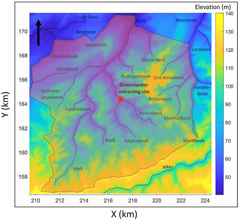
Figure 6. Digital elevation model of the study area with the river network and the delimitation of the boundaries.
In the South of the study area, the hill ridge serves as the southern boundary of the model. It is considered as a groundwater divide with the adjacent catchment. It can thus be characterized by a zero-flux crossing the boundary (Neumann boundary condition). The western boundary follows a spur of the southern hill ridge and is thus also assigned a zero-flux boundary. From this ridge, the boundary continues perpendicularly toward the Melsterbeek (Figure 6). Along this segment, the water flow direction will be mostly directly toward the river, with limited amount of water crossing the boundary and a zero-flux boundary type is therefore assigned. The Melsterbeek and the Bergbeek are two streams forming the rest of the western boundary. Here a specified hydraulic head is assigned, 1 m below the topography, assuming that the aquifer is in equilibrium with the river. Although the water level can change slightly from year to year, these rivers are located far from the extraction area and these variations are assumed negligible. For the northern and eastern boundary, a similar approach following streams and rivers (Bergbeek, Spaasbeek, Herk River, Kleine Herk, and Mombeek) joined by perpendicular segments is followed, assigning, respectively, fixed hydraulic heads and zero-flux boundary conditions (Figure 6). The hill ridge between the Herk and the Mombeek was considered too close to the extraction site to be used as a boundary. From the Source of the Mombeek a spur of the hill ridge is followed until the southern boundary is reached. The boundary conditions remain the same for all stress periods used in the model.
For the Cretaceous layers forming the semi-confined aquifer, there is a regional groundwater flow component from the South-East to North-West, so that other boundary conditions must be implemented. The regional flow is extracted from the primary monitoring network of the Flemish Environmental Agency (VMM) and specified heads are used along the north-western and south-eastern boundaries. The north-eastern and south-western boundaries are parallel to the regional flow and are thus set as zero-flux boundaries.
River Network
The model area is located in the catchment of the Herk river between the Mombeek and the Melsterbeek. Several smaller streams also cut into the landscape. The water extraction site is located around the point where the Molenbeek flows into the Herkebeek. The latter flows into the Herk (Figure 6), which in turn flows into the Demer north of the study area. All rivers and streams in the study area flow toward the lower lying areas in the North (Figure 6). Based on observations, the streams within the study area are relatively shallow and the rivers are therefore implemented as head-dependent flux boundaries (river package). This type of boundary allows an exchange between the aquifer and the river, dependent on the head calculated in the aquifer. The magnitude of this flow is regulated by the conductance factor, which describes the resistance of water flow between the river and the adjacent cells. This factor is in function of the thickness and hydraulic conductivity of the riverbed and the width and length of the river in the cell (Harbaugh, 2005).
Wells
The different pumping wells were implemented using the well-package. The pumping rates at the water extraction site in Voort vary between the different wells and between different stress periods. Wells 4017-001 overall has the highest pumping rate with an average of 915 m3/day. This is followed by pumping wells 4017-002 and 4017-004 which pump at an average rate of 692 and 669 m3/day, respectively. Lastly, pumping well 4017-003 has the lowest pumping rate with an average of 433 m3/day. North of Voort, in Wellen, another extraction site is present with two pumping wells, which are never active simultaneously. The average pumping rate of this water extraction site is 1,773 m3/day.
Recharge and Drainage
Estimating the recharge is difficult because of many local variations. For the Cretaceous aquifer itself, the recharge zone is located outside the study area to the South where the corresponding formations are outcropping, and an incoming flux is determined by the boundary conditions. For the upper layers, the recharge is coming from rainfall. The total estimated yearly recharge is 198 mm/year (Driesen, 1980), calculated as the difference between the precipitation and the annual evaporation. The latter was calculated using the Coutagne formula (Coutagne, 1954). The recharge is homogeneously distributed in the model and kept constant for the different stress-period. There is no evidence that the presence of the fracture zones in the Cretaceous aquifer have an impact on the recharge patterns, likely because the recharge from precipitation is dominated by the topography and the surface deposits, which are relatively homogeneous. Indeed, part of the recharge is immediately drained by small streams and rivers, as well as through small drains and ditches that are present in the study area. The latter are impossible to model individually. A drainage level was therefore implemented in the model. A linear relationship was derived between the elevation and the depth of the water level in the Quaternary aquifers using shallow piezometers available in the study area and was set as the drainage level. These observation wells are available from the monitoring done by De Watergroep around the pumping wells and from the monitoring network from VMM, from which freely accessible data is available. In consequence, the effective recharge to the model is the difference between the recharge from rainfall and the water drained from the aquifer. The latter is governed by the drainage base and the conductance factor set to 100 m2/day. This approach allows us to simplify the process taking place in the unsaturated zone and at the surface and avoid the complexity of a fully integrated model.
Hydraulic Conductivity
Before calibration, the horizontal and vertical hydraulic conductivities for each of the nine layers of the groundwater were estimated (Table 1). The most sensitive parameters are those from the Cretaceous from which water is extracted (layers 8 and 9). Although data from the Flemish database show local variations in the hydraulic parameters for the different layers, all the layers were considered as homogeneous for the calibration, with initial values taken from the literature (e.g., Calembert, 1956; Maréchal, 1993; Wouters and Vandenberghe, 1994; Diez, 1999; Feyen et al., 1999; Corluy et al., 2004; Lebbe and Vandenbohede, 2004; Vandersteen et al., 2014). A constant ratio of 10 between the horizontal and vertical hydraulic conductivity is kept for all further simulations.

Table 1. Initial horizontal and vertical hydraulic conductivity of the cretaceous.
Initial Head
For layer 1 to 7, the initial head is set equal to the drainage level. A first simulation is run for the first stress period (no pumping) with this initial head. The computed hydraulic heads are then used as initial head values for subsequent simulations. This allows to already integrate the effect of rivers in the initial head distribution.
In the Cretaceous (layers 8 and 9), the initial heads are based on an existing piezometric map of the Cretaceous aquifer generated by interpolating the available measured hydraulic heads in the Formations of Maastricht and Gulpen using kriging (VMM, 2008). This distribution is in accordance with the boundary conditions.
Fracture Zones
Several scenarios (Figure 7) are tested to implement the fractured zones detected by ERT in the groundwater model. In the original scenario A, only the main fractured zones observed in the center of the model are implemented. In scenario B, also the fractured zones detected on the crests and hill slopes are integrated. The other scenarios are assuming that the detected fractured zones are present in the whole model domain, even if ERT data were only available in the center. Scenarios C is similar to scenario A but with the fracture zone extending to the edges of the model. Scenario D is similar to scenario C but with another orientation of the fractures. Scenario E is similar to scenario C but with a unique larger fractured zone instead of 3 smaller ones. Scenario F uses an even larger fracture zones. Finally, scenario G has 3 relatively large fractured zones across the whole model corresponding to the groups of fractures detected by ERT. In the fracture zones, the hydraulic conductivity of the cells of layer 8 (Maastricht Formations) is increased in order to accommodate the fact that water is flowing more easily in the fracture zones.
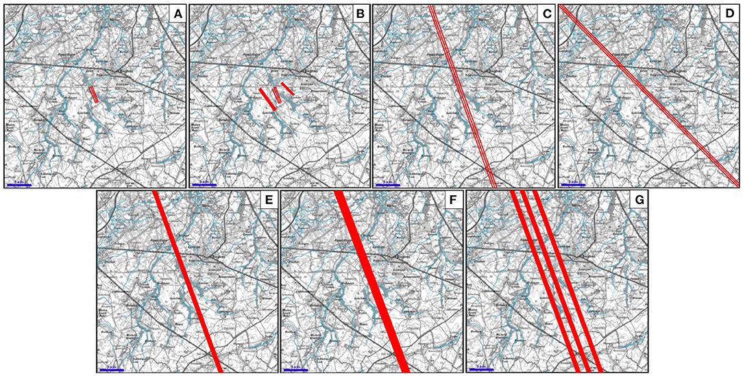
Figure 7. (A–G) Scenarios for the implementation of fractured zones in the model. See the text for the description of the specific scenarios.
Although adding anisotropy to characterize flow in faults and fractures is a common approach (Bear, 1993; Medici et al., 2021), the hydraulic conductivity of the fracture zones is modeled as isotropic. This approach is justified because fractures are not modeled individually, but globally as wider zones, and because the contrast of hydraulic conductivity between fractured zones and the background combined with the geometry of the fractured zones is sufficient to simulate preferential flow path along the direction of the fracture.
Results
Calibration
First, a calibration of the homogeneous model was performed to estimate the hydraulic conductivity of the different layers. The best model fitting was obtained with the parameters of Table 2. In Table 3, the results of different calibration attempts are shown in terms of average misfit (difference between observed and calculated hydraulic heads throughout the time series) for selected monitoring wells located both in the Cretaceous and in the upper layers as well as the maximum drawdown observed in the pumping wells. The objectives being to both reproduce correctly the observed distribution of hydraulic head through time and to correctly estimate the cone of depression resulting from pumping activities.
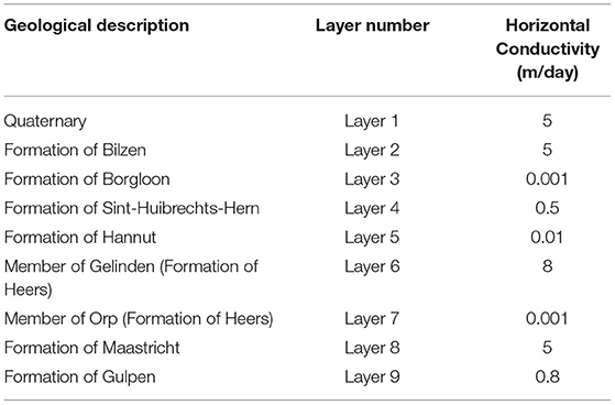
Table 2. Calibrated hydraulic conductivity for the homogeneous case.
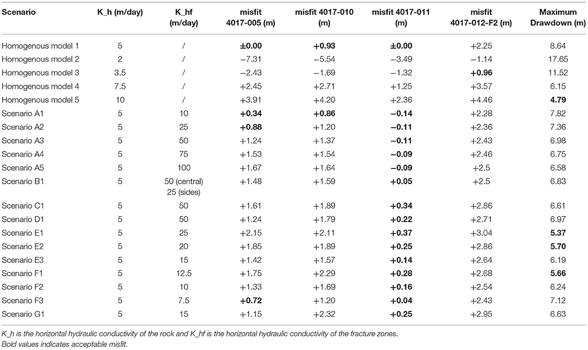
Table 3. Calibration of the different scenarios.
Note that a perfect fit is not expected as the simulations calculate yearly average water levels using average extraction rates while the data set is made of monthly measurements capturing seasonal variations and variations in the extraction rate. In addition, the size of the model is such that the grid size is not sufficient to accurately simulate individual drawdowns as some strong variations are sometimes observed at short distances. Moreover, pumping wells are affected by clogging, so that the measured hydraulic heads are lower than the actual levels in the aquifer.
The results of calibration of the homogeneous case (Table 3, Figure 8) show that it is very difficult to obtain at the same time an acceptable calibration in all observation wells and a realistic prediction of the maximum drawdown at the pumping wells that should be below 6 m. Although an underestimation of the drawdown at the pumping wells is expected with the model given the averaging effect of the grid size and the clogging of the well, the homogeneous model tends to overestimate this drawdown, clearly indicating an underestimation of the hydraulic head. Some trends observed in the piezometers are also not captured by the model (Figure 8), probably because they result from factors external to the extraction site and are not accounted for in the model (change in the boundary conditions or the recharge rate).
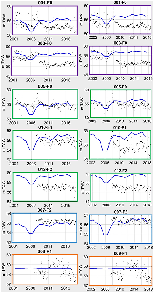
Figure 8. Calibration results for the homogeneous case (left) and scenario E3 (right). The dots show the monthly hydraulic head measurements, the blue line is the simulated yearly hydraulic head. Explanation of color frames: purple, pumping well; green, formation of Maastricht; blue, Member of Orp; orange, Quaternary.
The best result is obtained with a horizontal hydraulic conductivity of 5 m/day for the formation of Maastricht, but the model is highly sensitive to variations of this model parameter. An increase in the hydraulic conductivity of the layer allows to better match the drawdown in the wells, but at the expense of the fit in the monitoring wells, making it impossible to fulfill the two above-mentioned objectives with a homogeneous chalk layer.
Following this reasoning, it seemed that implementing fractured zones with a higher hydraulic conductivity should help to better fit the observed data. The different scenarios involving fracture zones were implemented in the model (Table 3). The hydraulic conductivity of the layer was kept as the one from calibration of the homogeneous case (5 m/day) while the fractured zones were assigned a larger hydraulic conductivity. Globally, adding the fractured zones allowed to better balance between the two objectives of fitting the maximum drawdown in the pumping wells while properly estimating the water level in the monitoring wells. Adding the fractures also improved the fit for wells located in the Member of Orp (layer 7), while the Quaternary layer (layer 1) was not really affected (Figure 8).
From scenarios A (Table 3), it is clear that increasing the hydraulic conductivity of the implemented fractured zones allowed to better fit the drawdown in the well. While the fit in the monitoring wells is degrading, this is not as bad as in the homogeneous case, indicating that including fractures in the model is an efficient way to obtain a better fit. The other proposed scenarios for the inclusion of fractures have only a limited impact on the model misfit. This is likely related to the absence of monitoring wells outside of the center of the model where the main fractures zones where detected using ERT. Nevertheless, since fractured zones are likely not limited to the center of the model, we found interesting to study those alternatives. Globally, they allow to further improve the maximum estimation of the drawdown in the pumping wells, without adding a negative effects on the monitoring wells. A good compromise is found for scenario E3, with a unique, wide fractured zone with a hydraulic conductivity 3 times larger than the homogeneous layer (Figure 8), although it remains difficult to select the best solution given the two conflicting objectives. The quality of calibration is considered as sufficient to investigate the impact of new exploitation scenarios on the drawdown in the catchment. The model of scenarios E3 is kept as a basis for predictive purposes.
New Exploitation Scenarios
In the management strategy of De Watergroep, the extraction rate in the catchment should be increased from 2,600 m3/day to about 6,000 m3/day. Two scenarios are envisaged: (1) increasing the pumping rate of the current wells, (2) drilling a new well in the catchment. For the second choice, the options are limited. To limit the investment costs, the only viable solution is to drill a well next to an existing water reservoir owned by de Watergroep (Figure 9). This reservoir is located on the crest along ERT profile 2. On this profile, a fractured zone was detected, with very low resistivity, and a second possible fractured zone was identified with a less significant contrast in resistivity. Since the water reservoir is located on top of the latter, this option was retained in the simulation scenarios. However, given the limited contrast in resistivity, we expect the hydraulic conductivity to be only slightly larger in the fracture zone.
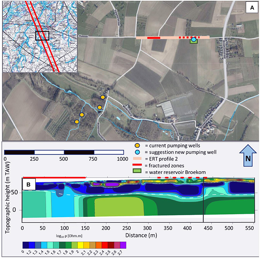
Figure 9. Location of the new pumping well-based on ERT. (A) Aerial view of the study area. (B) Location of the well on the ERT profile.
The objective of the prediction is to estimate the hydraulic head in the Cretaceous layer and the maximum drawdown in the Quaternary. The former will determine the new protection zone around the pumping wells, while the latter is significant for geotechnical considerations. Indeed, the Quaternary layer contains peat, and an excessive drawdown could yield some subsidence and differential settlement in the area. In particular, we analyse the impacts of the conceptualization choices on the model prediction. In other words, we assume that a model including the fracture zones detected by ERT is more appropriate, and estimate how an error in the conceptualization propagates in the model prediction. This is justified as the calibration of the model with a homogeneous chalk aquifer yielded an overestimation of the drawdown and the hydraulic gradient, and therefore an overestimation of the settlement in the Quaternary layer.
Four scenarios are tested (Table 4). Scenario 1 considers the current pumping rate. Scenario 2 considers an increase of the pumping rate using the current wells. Scenario 3 considers a new pumping well-ignoring the fractured zones detected by ERT, with the total pumping rate equally distributed over the 5 wells. Finally, scenarios 4a to 4d considers that the new pumping well is located in a fractured zone, as identified by the ERT results, with increasing hydraulic conductivity. The results are summarized in Figure 10 and Table 4.
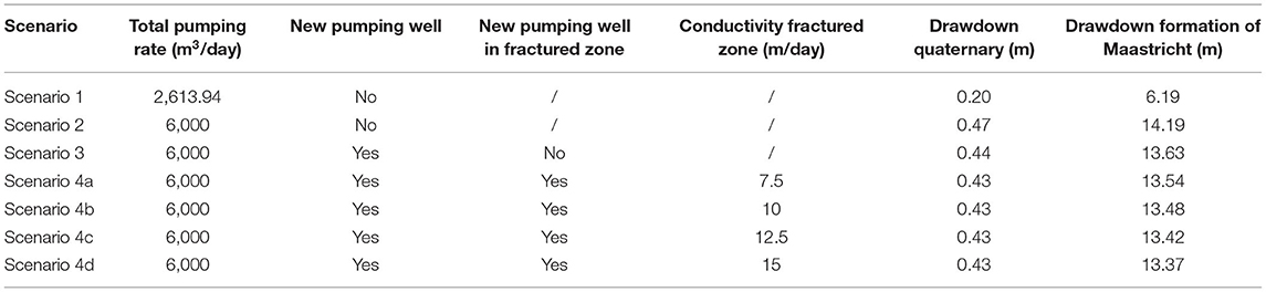
Table 4. Drawdowns calculated for the tested scenarios.
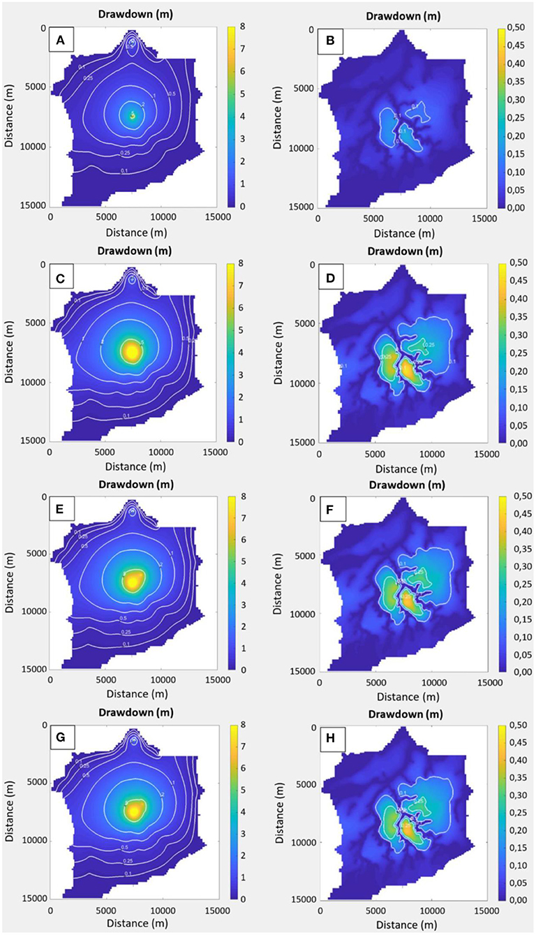
Figure 10. (A) Drawdown in the formation of Maastricht (layer 8) in scenario 1 (Table 4). (B) Drawdown in the Quaternary (layer 1) in scenario 1. (C) Drawdown in the formation of Maastricht in scenario 2. (D) Drawdown in the Quaternary in scenario 2. (E) Drawdown in the formation of Maastricht in scenario 3. (F) Drawdown in the quaternary in scenario 3. (G) Drawdown in the formation of Maastricht in scenario 4d. (H) Drawdown in the quaternary in scenario 4d.
With the current pumping rate (Scenario 1), the simulated maximum drawdown in the Cretaceous layers is about 6.2 m, and is 0.2 m in the Quaternary layer. When increasing the pumping rate (Scenario 2), those maximum drawdown increase to 14.19 m and 0.47 m, respectively. Allocating 20% of the extraction rate to a new well located on the crest (Scenario 3), reduces the maximum drawdown in the Cretaceous layer to 13.63 and 0.44 m in the Quaternary layer and significantly reduces the area impacted by large drawdowns (Figure 10). The maximum drawdown remains of course located under the current well-battery, and reducing further the observed drawdown would require to allocate a higher extraction rate to the new wells. In consequence, the presence or absence of a fractured zone only has a limited impact on the maximum drawdown in both studied layers in the new pumping well. However, the drawdown in the new pumping well is significantly reduced from 8 to 6.5 m. Therefore, a better repartition of the extraction rate within the fractured zones detected by ERT would be a reasonable management scenario for this catchment in order to limit the maximum drawdowns observed in the aquifer and overlying layers.
Discussion
The improvement in the calibration obtained by implementing some fractured zones is expected as adding additional conductivity zones increases the degree of freedom in the parameter space what should always allow to obtain a better fit. In addition, the sparse ERT data do not allow to unequivocally delimit the fractured zone extension, both in length and width, and the resolution of the model is insufficient to accurately translate the geophysical findings into the groundwater model. One could thus argue that an approach based on geophysical data is not necessary and that similar results could be obtained through a spatially-distributed calibration approach such as the pilot-point method (e.g., Christensen et al., 2016) or through a more explorative approaches using the expected orientation of the fractures (Figure 5B). Based on such prior geological knowledge, one would have likely generated a situation similar to scenario E or F, with a fracture zone in the center of the valley, as this was the original assumption, and would have achieved similar results in terms of calibration.
However, we strongly believe that such a blind increase of the complexity of the model should be avoided. In this specific case, the ERT data have falsified the initial assumption that fractured zones were limited to the center of the valleys. Although this observation has limited impact on the calibration of the model, because the majority of the monitoring piezometers are located close to the pumping wells, it has huge implications for the stakeholders for the development of future management scenarios: new pumping wells should be preferentially drilled in fractured zones to reduce as much as possible the drawdown in the aquifer, while maintaining an economically sufficiently high pumping rate. Therefore, adding K zones not defined by geophysics, would indeed improve the fit in a similar way, because the conceptualization is very similar, but would not allow to make wise choices for the future management of the extraction site. The added value of geophysical data therefore goes beyond the calibration itself and allow to increase the confidence in the model results for stakeholders (e.g., Ferré, 2017).
Although several attempts were made—such as including anisotropy in the hydraulic conductivity along the fractured zones, increasing further their hydraulic conductivity, modifying their geometry or increasing the number of fractured zones—further improvement of the model calibration was not achieved. The results of Table 3 tends to indicate that fractures indeed play an important role in the distribution of the drawdowns around the pumping wells. However, the overall fit of the temporal trend in the data remains poor and obtaining a better fit would require, on one hand, a description of the fracture zones at a better resolution, with more ERT profiles allowing to clearly image the geometry of the zones, and a refinement of the model grid in order to properly integrate this geometry in the model; and on the other hand, an analysis of the temporal variability of the recharge and boundary conditions.
An extended uncertainty analysis including such more advanced models would help to objectify the improvement brought by the ERT data in the conceptualization of the heterogeneity of the aquifer, and to estimate if this improvement is statistically meaningful. Such a study falls out of the scope of this paper. Based on our analysis, the overestimation of the drawdown at the pumping well with the homogeneous case seems to indicate that the wells are located in a fractured zone with a larger hydraulic conductivity. This is corroborated by the ERT profile 1 for which one of the pumping well is located near a low resistivity zone. However, since the available data are mostly located in the center of the model, the higher model complexity would not necessarily improve the predictive capability of the model outside of the pumping zone.
Given the (semi-)confined nature of the aquifer, the relative homogeneity of the surface layers, and the objectives of the study, it was possible to simplify the conceptualization of the subsurface by modeling infiltration through the unsaturated zone as a constant recharge rate and to focus on the groundwater component of the system. However, field observations such as seepage in some areas of the study area and the role of drains and streams are pointing toward a complex subsurface system where interactions with surface water and the unsaturated zone play an important role. At this stage, developing a fully integrated model is premature given the lack of data in the catchment. A first step would be to better model the run-off, evapotranspiration and recharge by using a spatially distributed model of the soil layer and land occupation, coupled with a fully transient approach. For such a model, ERT data could also play an important role in identifying the heterogeneity in the shallow layers as shown in Figure 4. Several studies have also demonstrated the added value of ERT data in monitoring the water content in the unsaturated zone during infiltration experiments, allowing to better estimate essential parameters related to the unsaturated zone (e.g., Claes et al., 2019, 2020; Blazevic et al., 2020). Long-term experiments at the catchment scale have also shown the ability of ERT to monitor seasonal variations in the water content, allowing to better model recharge in aquifers (Kuhl et al., 2018; Kotikian et al., 2019). However, for logistical reasons, 4D ERT surveys are generally limited to the local scale and difficult to apply to large catchments (Uhlemann et al., 2017).
Conclusion
Fractured aquifers are particularly complex to model because of the presence of preferential flow paths that are difficult to identify from well-data only. In this contribution, we used electrical resistivity profile to characterize a fractured chalk aquifer in Voort, Belgium. The ERT data clearly identifies the presence of lower resistivity zones, that are interpreted as zones of higher water content because of the presence of secondary porosity (fractures). In contrast to preliminary assumptions, the fractured zones were not only located in topographical depressions, but also along hillslopes and crests. The NW-SE orientation of these fractures zones seemed in accordance with the regional tectonic context (Roer Graben).
The information brought by geophysical methods appeared to be essential in the groundwater modeling process. A model with homogeneous layers was not able to explain both the hydraulic head in monitoring wells and the observed drawdown in pumping wells. Adding the identified fractured zones with higher hydraulic conductivity values in the model allowed to globally reduce the misfit of the model and to increase the confidence in its predictive capability. Nevertheless, a more detailed characterization of the geometry of the fractures combined with a higher resolution groundwater model would be necessary in order to obtain a better characterization. This was not considered essential given the objectives of the study.
Although similar calibration results could have been obtained based on a simple conceptualization of fracture zones, the ERT data help to increase the overall confidence in the model output, as the proposed approach is data-driven, especially for model prediction. Indeed, while testing future management scenarios for the extraction site, the knowledge of the location of fractured zone appeared to be crucial. The model showed that distributing the extraction rate among several fractured zones is likely the best option to minimize the maximum drawdown in the aquifer and shallow layers. This prediction should be further validated when new data will become available in the catchment.
This study demonstrated the usefulness of acquiring geophysical data at the catchment scale. Although the coverage was limited, the ERT field campaign performed in two periods allowed to identify the fracture zones in the study area and their orientation, allowing to significantly improve our conceptual understanding of the hydrogeological system.
Data Availability Statement
The datasets presented in this article are not readily available because the monitoring groundwater data of the extraction site are confidential data of De Watergroep. A motivated request for accessing the data can be sent to Alexander.Vandenbohede@dethwatergroep.be or simon.six@dewatergroep.be and will be reviewed in due time. The geophysical data generated for this study can be obtained upon request by contacting the corresponding author. Requests to access the datasets should be directed to thomas.hermans@ugent.be; Alexander.Vandenbohede@dethwatergroep.be; simon.six@dewatergroep.be.
Author Contributions
BV: fieldwork, data processing, modeling, interpretation, and manuscript draft. SS: fieldwork, conceptualization, supervision, and manuscript proofreading. KW: conceptualization, supervision, and manuscript proofreading. AV: fieldwork, modeling, interpretation, and manuscript proofreading. TH: fieldwork, conceptualization, data processing, interpretation, supervision, and manuscript draft. All authors contributed to the article and approved the submitted version.
Conflict of Interest
AV and SS are employed by De Watergroep, a public company responsible for the production of drinking water in Flanders. BV is now employed by Antea Group, but was affiliated to Ghent University during the study.
The remaining authors declare that the research was conducted in the absence of any commercial or financial relationships that could be construed as a potential conflict of interest.
Publisher's Note
All claims expressed in this article are solely those of the authors and do not necessarily represent those of their affiliated organizations, or those of the publisher, the editors and the reviewers. Any product that may be evaluated in this article, or claim that may be made by its manufacturer, is not guaranteed or endorsed by the publisher.
Acknowledgments
We thank Liege University (Prof. F. Nguyen) for lending us the ERT equipment. We thank Christian Rummens and Toon Van Dijck from De Watergroep, and Marieke Paepen from Ghent University for their help on the field. We also thank the Associated Editor Marc Leblanc, Ty Ferré, and Ulrich Ofterdinger for their comments that helped to improve the quality of the manuscript.
References
Al-Tarazi, E., El-Naqa, A., El-Waheidi, M., and Abu Rajab, J. (2006). Electrical geophysical and hydrogeological investigations of groundwater aquifers in Ruseifa municipal landfill, Jordan. Environ. Geol. 50, 1095–1103. doi: 10.1007/s00254-006-0283-4
Barfod, A. A. S., Vilhelmsen, T. N., Jørgensen, F., Christiansen, A. V., Høyer, A.-S., Straubhaar, J., et al. (2018). Contributions to uncertainty related to hydrostratigraphic modeling using multiple-point statistics. Hydrol. Earth Syst. Sci. 22, 5485–5508. doi: 10.5194/hess-22-5485-2018
Bear, J. (1993). Modelling Flow and Contaminant Transport in Fractured Rocks. Oxford: Academic Press, 1–37. doi: 10.1016/B978-0-12-083980-3.50005-X
Berkowitz, B. (2002). Characterizing flow and transport in fractured geological media: A review. Adv. Water Resour. 25:861–884. doi: 10.1016/S0309-1708(02)00042-8
Binley, A., Hubbard, S. S., Huisman, J. A., Revil, A., Robinson, D. A., Singha, K., et al. (2015). The emergence of hydrogeophysics for improved understanding of subsurface processes over multiple scales. Water Resourc. Res. 51, 3837–3866. doi: 10.1002/2015WR017016
Blazevic, L. A., Bodet, L., Pasquet, S., Linde, N., Jougnot, D., and Longuevergne, L. (2020). Time-Lapse seismic and electrical monitoring of the vadose zone during a controlled infiltration experiment at the ploemeur hydrological observatory, France. Water 12:1230. doi: 10.3390/w12051230
Cadée, M. C. (1991). Het oligoceen en de oligocene mollusken fauna's van nederland en omgeving. Afzettingen 1, 3–19.
Calembert, L. (1956). Le Crétacé Supérieur De La Hesbaye Et Du Brabant. Ann. Soc. Géol. Belgi. 80, 129–156.
Caterina, D., Beaujean, J., Robert, T., and Nguyen, F. (2013). A comparison study of different image appraisal tools for electrical resistivity tomography. Near Surf. Geophysics 11, 639–657. doi: 10.3997/1873-0604.2013022
Cheng, Q., Chen, X., Tao, M., and Binley, A. (2019). Characterization of karst structures using quasi-3D electrical resistivity tomography. Environ. Earth Sci. 78:285. doi: 10.1007/s12665-019-8284-2
Christensen, N. K., Christensen, S., and Ferre, T. P. A. (2016). Testing alternative uses of electromagnetic data to reduce the prediction error of groundwater models. Hydrol. Earth Syst. Sci. 20, 1925–1946. doi: 10.5194/hess-20-1925-2016
Claes, N., Paige, G. B., Grana, D., and Parsekian, A. D. (2020). Parameterization of a hydrologic model with geophysical data to simulate observed subsurface return flow paths. Vadose Zone J. 19:e20024. doi: 10.1002/vzj2.20024
Claes, N., Paige, G. B., and Parsekian, A. D. (2019). Uniform and lateral preferential flows under flood irrigation at field scale. Hydrol. Process. 33, 2131–2147. doi: 10.1002/hyp.13461
Claes, S., and Willems, D. (1997). Tertiairgeologische Kaart Van België. Kaartblad 33-41 Sint-Truiden. Adobe Acrobat (pdf) file, schaal 1:50,000. Available online at: https://www.vlaanderen.be/publicaties/tertiairgeologische-kaart-van-belgi-kaartblad-33-41-sint-truiden
Cong-Thi, D., Dieu, L. P., Thibaut, R., Paepen, M., Ho, H. H., Nguyen, F., et al. (2021). Imaging the structure and the saltwater intrusion extent of the luy river coastal aquifer (Binh Thuan, Vietnam) using electrical resistivity tomography. Water. 13, 1743. doi: 10.3390/w13131743
Corluy, J., Verbeiren, B., Batelaan, O., and De Smedt, F. (2004). “Integrating vegetation mapping in groundwater modelling for ecohydrological predictions within an ecosystem vision. Model application for wetlands hydrology and hydraulics,” in Center of Excellence in Wetland Hydrology, WETHYDRO, eds J. Kubrak, T. Okruszko, and S. Ignar (Warsaw: Warsaw Agricultural University Press), 155–166.
Coutagne, A. (1954). Quelques considérations sur le pouvoir évaporant de l'atmosphère, le déficit d'écoulement effectif et le déficit d'écoulement maximum. La Houille Blanche 6, 360–369. doi: 10.1051/lhb/1954036
Dahlin, T., and Zhou, B. (2006). Multiple-gradient array measurements for multichannel 2D resistivity imaging. Near Surf. Geophys. 4, 113–123. doi: 10.3997/1873-0604.2005037
De Bast, E., Steurbaut, E., and Smith, T. (2013). New mammals from the marine Selandian of Maret, Belgium, and their implications for the age of the paleocene continental deposits of Walbeck, Germany. Geol. Belg. 16, 236–244. Available online at: https://popups.uliege.be/1374-8505/index.php?id=4267
De Geyter, G. (1988). “Formatie van Hanut,” in Voorstel Lithostratigrafische Indeling Van Het Paleogeen, eds R. Maréchal, and P. Laga (Brussel: Belgische Geologische Dienst), 60–71.
De Watergroep (2014). Vijfjaarlijks Verslag Grondwaterwinning Voort. Brussels, Belgium: De Watergroep.
Deckers, J., Broothaers, M., Lagrou, D., and Matthijs, J. (2014). The late Maastrichtian to Late Paleocene tectonic evolution of the southern part of the Roer Valley Graben (Belgium). Netherl. J. Geosci. Geol. Mijnbouw 93, 83–93. doi: 10.1017/njg.2014.11
Deckers, J., Van Noten, K., Schiltz, M., Lecocq, T., and Vanneste, K. (2018). Integrated study on the topographic and shallow subsurface expression of the Grote Brogel Fault at the boundary of the Roer Valley Graben, Belgium. Tectonophysics 722, 486–506. doi: 10.1016/j.tecto.2017.11.019
Diez, T. (1999). Hydrogeologische Studie Van Het Gebied Rond de Site Van Montenaken - Zevenbronnen. (Master's thesis), KULeuven, Leuven (Belgium).
DOV. (2019). Krijt Isohypsen, Isopachen en Breuken. Databank Ondergrond Vlaanderen, Vlaamse Overheid. Available online at: https://www.dov.vlaanderen.be/portaal/?module=verkenner&pos=140500%2C200000&res=140.00000000044093&layers=n%3Aomwrgbmrvl%3Bo%3Aref%2Cn%3Agrb_sel%3Bo%3Aref%2Cn%3Ato%5C%3Ato_topnzw_2009_raster_10k_tr%3Bo%3Aref%3Bt%3Awms%3Bv%3An%2Cn%3Adov-pub%5C%3AKrijt_Isopachen%3Bo%3Adov%3Bt%3Awms%3Bv%3An%2Cn%3Adov-pub%5C%3AKrijt_Isohypsen_Basis%3Bo%3Adov%3Bt%3Awms%3Bv%3An%2Cn%3Adov-pub%5C%3AKrijt_Breuken_Basis%3Bo%3Adov%3Bt%3Awms%3Bv%3An%2Cn%3Adov-pub%5C%3AKrijt_Breuken_Top%3Bo%3Adov%3Bt%3Awms%2Cn%3Adov-pub%5C%3AKrijt_Isohypsen_Top%3Bo%3Adov%3Bt%3Awms
Driesen, L. (1980). Hydrogeologische Studie van de Secundaire Formaties in Zuid-Limburg. (Master's thesis), KULeuven, Leuven (Belgium).
Ferré, T. P. A. (2017). Revisiting the relationship between data, models, and decision-making. Groundwater 55, 604–614. doi: 10.1111/gwat.12574
Feyen, L., Vazquez, R., Christiaens, K., Sels, O., and Feyen, J. (1999). Kalibratie- en validatieprocedure van het ruimtelijk verdeeld fysisch gebaseerd hydrologische MIKE 68 SHE-model met toepassing op het stroomgebied van de grote en de Kleine Gete. Tijdschrift Water 101, 21–41.
Gallegos, J. J., Hu, B. X., and Davis, H. (2013). Simulating flow in karst aquifers at laboratory and sub-regional scales using MODFLOW-CFP. Hydrogeol. J. 21, 1749–1760. doi: 10.1007/s10040-013-1046-4
Guérin, R. (2005). Borehole and surface-based hydrogeophysics. Hydrogeol. J. 13, 251–254. doi: 10.1007/s10040-004-0415-4
Guérin, R., Baltassat, J.-M., Boucher, M., Chalikakis, K., Galibert, P. Y., Girard, J.-F., et al. (2009). Geophysical characterisation of karstic networks–application to the ouysse system (Poumeyssen, France). Compt. Rendus Geosci. 341, 810–817. doi: 10.1016/j.crte.2009.08.005
Guevara-Mansilla, O., López-Loera, H., Ramos-Leal, J. A., Ventura-Houle, R., and Guevara-Betancourt, R. E. (2020). Characterization of a fractured aquifer through potential geophysics and physicochemical parameters of groundwater samples. Environ. Earth Sci. 79:352. doi: 10.1007/s12665-020-09096-y
Harbaugh, A. W. (2005). Groundwater MODFLOW-2005, The U.S. Geological Survey Modular Ground-Water Model–The Ground-Water Flow Process: U.S. Geological Survey Techniques and Methods. Reston, VA: USGS Publications Warehouse. doi: 10.3133/tm6A16
Hill, M. E., Stewart, M. T., and Martin, A. (2010). Evaluation of the MODFLOW-2005 conduit flow process. Groundwater 48, 549–559. doi: 10.1111/j.1745-6584.2009.00673.x
Katika, K., Alam, M. M., Alexeev, A., Chakravarty, K. H., Fosbøl, P. L., Revil, A., et al. (2018). Elasticity and electrical resistivity of chalk and greensand during water flooding with selective ions. J. Petrol. Sci. Eng. 161, 204–218. doi: 10.1016/j.petrol.2017.11.045
Knight, R., Smith, R., Asch, T., Abraham, J., Cannia, J., Viezzoli, A., et al. (2018). Mapping aquifer systems with airborne electromagnetics in the central valley of California. Groundwater 56, 893–908. doi: 10.1111/gwat.12656
Kotikian, M., Parsekian, A. D., Paige, G., and Carey, A. (2019). Observing heterogeneous 1076 unsaturated flow at the hillslope scale using time-lapse electrical resistivity tomography 1077. Vadose Zone J. 18, 1–16. doi: 10.2136/vzj2018.07.0138
Kuhl, A. S., Kendall, A. D., Van Dam, R. L., and Hyndman, D. W. (2018). Quantifying soil water and root dynamics using a coupled hydrogeophysical inversion. Vadose Zone J. 17, 1–13. doi: 10.2136/vzj2017.08.0154
LaBrecque, D. J., Miletto, M., Daily, W., Ramirez, A., and Owen, E. (1996). The effects of noise on Occam's inversion of resistivity tomography data. Geophysics 61, 538–548. doi: 10.1190/1.1443980
Laga, P. (1988). “Formatie van sint-huibrechts-Hern,” in Voorstel Lithostratigrafische Indeling Van Het Paleogeen, eds R. Maréchal, and P. Laga (Brussel: Belgische Geologische Dienst), 164–169.
Laga, P., Louwye, S., and Geets, S. (2001). Paleogene and Neogene lithostratigraphic units (Belgium). Geologica Belgica 4, 135–152.
Lebbe, L., and Vandenbohede, A. (2004). Ontwikkeling Van Een Lokaal Axi-Symmetrisch Model Op Basis Van De HCOV Kartering Ter Ondersteuning Van De Adviesverlening Voor Grondwaterwinningen. Studie in Opdracht Van AMINAL, Afdeling Water. Ghent: UGent.
Lemieux, J. M., Therrien, R., and Kirkwood, D. (2006). Small scale study of groundwater flow in a fractured carbonate rock aquifer at the St-Eustache quarry, Québec, Canada. Hydrogeol. J. 14, 603–612.
Lesparre, N., Nguyen, F., Kemna, A., Robert, T., Hermans, T., Daoudi, M., et al. (2017). A new approach for time-lapse data weighting in electrical resistivity tomography. Geophysics 82, E325–E333. doi: 10.1190/geo2017-0024.1
Loke, M. H. (2006). RES2DINV Ver. 3.55. Rapid 2D Resistivity & IP Inversion Using the Least-Squares Method. Software Manual, 139.
Loke, M. H., Chambers, J. E., Rucker, D. F., Kuras, O., and Wilkinson, P. B. (2013). Recent developments in the direct-current geoelectrical imaging method. J. Appl. Geophys. 95, 135–156. doi: 10.1016/j.jappgeo.2013.02.017
Maillot, J., Davy, P., Le Goc, R., Darcel, C., and de Dreuzy, J. R. (2016). Connectivity, permeability, and channeling in randomly distributed and kinematically defined discrete fracture network models: permeability of discrete fracture network. Water Resourc. Res. 52, 8526–8545. doi: 10.1002/2016WR018973
Maréchal, R. (1993). A new lithostratigraphic scale for the Palaeogene of Belgium. Bull. Soc. Bel. Géol. 102, 215–229.
Masciopinto, C., Liso, I., Caputo, M., and De Carlo, L. (2017). An integrated approach based on numerical modelling and geophysical survey to map groundwater salinity in fractured coastal aquifers. Water 9:875. doi: 10.3390/w9110875
McDonald, M., and Harbough, A. W. (1988). A Modular Three-Dimensional Finite Difference Groundwater Flow Model. Reston, VA: U.S. Geological Survey.
Medici, G., Smeraglia, L., Torabi, A., and Botter, C. (2021). Review of modeling approaches to groundwater flow in deformed carbonate aquifers. Groundwater 59, 334–351. doi: 10.1111/gwat.13069
Medici, G., West, L. J., Mountney, N. P., and Welch, M. (2019). Permeability of rock discontinuities and faults in the Triassic Sherwood Sandstone Group (UK): insights for management of fluvio-aeolian aquifers worldwide. Hydrogeol. J. 27, 2835–2855. doi: 10.1007/s10040-019-02035-7
Mézquita González, J. A., Comte, J.-C., Legchenko, A., Ofterdinger, U., and Healy, D. (2021). Quantification of groundwater storage heterogeneity in weathered/fractured basement rock aquifers using electrical resistivity tomography: sensitivity and uncertainty associated with petrophysical modelling. J. Hydrol. 593:125637. doi: 10.1016/j.jhydrol.2020.125637
Miller, C. R., Routh, P. S., Brosten, T. R., and McNamara, J. P. (2008). Application of time-lapse ERT imaging to watershed characterization. Geophysics 73, G7–G17. doi: 10.1190/1.2907156
Minsley, B. J., Foks, N. L., and Bedrosian, P. A. (2021). Quantifying model structural uncertainty using airborne electromagnetic data. Geophys. J. Int. 224, 590–607. doi: 10.1093/gji/ggaa393
Molron, J., Linde, N., Baron, L., Selroos, J.-O., Darcel, C., and Davy, P. (2020). Which fractures are imaged with ground penetrating radar? Results from an experiment in the äspö hardrock laboratory, Sweden. Eng. Geol. 273:105674. doi: 10.1016/j.enggeo.2020.105674
Nelson, R. A. (1985). “Geologic analysis of naturally fractured reservoirs,” in Contributions Petroleum Geology & Engineering, Vol. 1. Houston, TX: Gulf Pub. Co., Book Division, 320 p.
Oldenburg, D. W., and Li, Y. (1999). Estimating depth of investigation in DC resistivity and IP surveys. Geophysics 64, 403–416. doi: 10.1190/1.1444545
Reninger, P.-A., Martelet, G., Lasseur, E., Beccaletto, L., Deparis, J., Perrin, J., et al. (2014). Geological environment of karst within chalk using airborne time domain electromagnetic data cross-interpreted with boreholes. J. Appl. Geophys. 106, 173–186. doi: 10.1016/j.jappgeo.2014.04.020
Revil, A., Coperey, A., Shao, Z., Florsch, N., Fabricius, I. L., Deng, Y., et al. (2017). Complex conductivity of soils. Water Resourc. Res. 53, 7121–7147. doi: 10.1002/2017WR020655
Ringel, L. M., Somogyvári, M., Jalali, M., and Bayer, P. (2019). Comparison of hydraulic and tracer tomography for discrete fracture network inversion. Geosciences 9:274. doi: 10.3390/geosciences9060274
Robert, T., Caterina, D., Deceuster, J., Kaufmann, O., and Nguyen, F. (2012). A salt tracer test monitored with surface ERT to detect preferential flow and transport paths in fractured/karstified limestones. Geophysics 77, B55–B67. doi: 10.1190/geo2011-0313.1
Robert, T., Dassargues, A., Brouyère, S., Kaufmann, O., Hallet, V., and Nguyen, F. (2011). Assessing the contribution of electrical resistivity tomography (ERT) and self-potential (SP) methods for a water well drilling program in fractured/karstified limestones. J. Appl. Geophys. 75, 42–53. doi: 10.1016/j.jappgeo.2011.06.008
Saller, S. P., Ronayne, M. J., and Long, A. J. (2013). Comparison of a karst groundwater model with and without discrete conduit flow. Hydrogeol. J. 21, 1555–1566. doi: 10.1007/s10040-013-1036-6
Schmutz, M., Ghorbani, A., Vaudelet, P., and Revil, A. (2011). Spectral induced polarization detects cracks and distinguishes between open- and clay-filled fractures. J. Environ. Eng. Geophys. 16, 85–91. doi: 10.2113/JEEG16.2.85
Slater, L., Binley, A. M., Daily, W., and Johnson, R. (2000). Cross-hole electrical imaging of a controlled saline tracer injection. J. Appl. Geophys. 44, 85–102. doi: 10.1016/S0926-9851(00)00002-1
Thorez, J., and Monjoie, A. (1973). Lithologie et assemblages argileux de la smectite de herve et des craies campaniennes et mastrichtiennes dans le nord-est de la belgique. Ann. Soc. Géol. Bel. 96, 651–670.
Travis, B. J. (1984). TRACR3D: A Model of Flow and Transport in Porous/fractured Media. Los Alamos, NM: Los Alamos National Laboratory.
Uhlemann, S., Chambers, J., Wilkinson, P., Maurer, H., Merritt, A., Meldrum, P., et al. (2017). Four-dimensional imaging of moisture dynamics during landslide reactivation. J. Geophys. Res. Earth Surf. 122, 398–418. doi: 10.1002/2016JF003983
Van Den Eeckhaut, M., Poesen, J., Dusar, M., Martens, V., and Duchateau, P. (2007). Sinkhole formation above underground limestone quarries: a case study in South Limburg (Belgium). Geomorphology 91, 19–37. doi: 10.1016/j.geomorph.2007.01.016
Van Hoorde, M., Hermans, T., Dumont, G., and Nguyen, F. (2017). 3D electrical resistivity tomography of karstified formations using cross-line measurements. Eng. Geol. 220, 123–132. doi: 10.1016/j.enggeo.2017.01.028
Vandenberghe, N., Van Simaeys, S., Steurbaut, E., Jagt, J. W. M., and Felder, P. J. (2004). Stratigraphic architecture of the upper cretaceous and cenozoic along the southern border of the North Sea Basin in Belgium. Netherl. J. Geosci. 83, 155–171. doi: 10.1017/S0016774600020229
Vandersteen, K., Gedeon, M., and Beerten, K. (2014). A synthesis of hydraulic conductivity measurements of the subsurface in Northeastern Belgium. Geol. Belg. 17, 196–210. Available online at: https://popups.uliege.be/1374-8505/index.php?id=4587
Vilhelmsen, T., Marker, P., Foged, N., Wernberg, T., Auken, E., Christiansen, A. V., et al. (2018). A regional scale hydrostratigraphy generated from geophysical data of varying age, type, and quality. Water Resourc. Manage. 33, 539–53. doi: 10.1007/s11269-018-2115-1
Wang, X., Jardani, A., Jourde, H., Lonergan, L., Cosgrove, J., Gosselin, O., et al. (2016). Characterisation of the transmissivity field of a fractured and karstic aquifer, Southern France. Adv. Wat. Res. 87, 106–121. doi: 10.1016/j.advwatres.2015.10.014
Yans, J., Spagna, P., Vanneste, C., Hennebert, M., Vandycke, S., Baele, J. M., et al. (2005). Description et implications geologiques preliminaires d'un forage carotte dans le “Cran aux guanodons” de Bernissart. Geol. Belg. 8, 43–49. Available online at: https://popups.uliege.be/1374-8505/index.php?id=531
Keywords: electrical resistivity tomography (ERT), fractures, chalk aquifer, groundwater model calibration, catchment scale
Citation: Van Riet B, Six S, Walraevens K, Vandenbohede A and Hermans T (2022) Assessing the Impact of Fractured Zones Imaged by ERT on Groundwater Model Prediction: A Case Study in a Chalk Aquifer in Voort (Belgium). Front. Water 3:783983. doi: 10.3389/frwa.2021.783983
Received: 27 September 2021; Accepted: 14 December 2021;
Published: 18 January 2022.
Edited by:
Marc Leblanc, University of Avignon, FranceReviewed by:
Ulrich Ofterdinger, Queen's University Belfast, United KingdomTy Ferre, University of Arizona, United States
Copyright © 2022 Van Riet, Six, Walraevens, Vandenbohede and Hermans. This is an open-access article distributed under the terms of the Creative Commons Attribution License (CC BY). The use, distribution or reproduction in other forums is permitted, provided the original author(s) and the copyright owner(s) are credited and that the original publication in this journal is cited, in accordance with accepted academic practice. No use, distribution or reproduction is permitted which does not comply with these terms.
*Correspondence: Thomas Hermans, thomas.hermans@ugent.be
†These authors have contributed equally to this work