 Siyan Liu
 Dan Lu
 Scott L. Painter
 Natalie A. Griffiths2
- 1Computational Sciences and Engineering Division, Oak Ridge National Laboratory, Oak Ridge, TN, United States
- 2Environmental Sciences Division, Oak Ridge National Laboratory, Oak Ridge, TN, United States
Machine learning (ML) models, and Long Short-Term Memory (LSTM) networks in particular, have demonstrated remarkable performance in streamflow prediction and are increasingly being used by the hydrological research community. However, most of these applications do not include uncertainty quantification (UQ). ML models are data driven and can suffer from large extrapolation errors when applied to changing climate/environmental conditions. UQ is required to quantify the influence of data noises on model predictions and avoid overconfident projections in extrapolation. In this work, we integrate a novel UQ method, called PI3NN, with LSTM networks for streamflow prediction. PI3NN calculates Prediction Intervals by training 3 Neural Networks. It can precisely quantify the predictive uncertainty caused by the data noise and identify out-of-distribution (OOD) data in a non-stationary condition to avoid overconfident predictions. We apply the PI3NN-LSTM method in the snow-dominant East River Watershed in the western US and in the rain-driven Walker Branch Watershed in the southeastern US. Results indicate that for the prediction data which have similar features as the training data, PI3NN precisely quantifies the predictive uncertainty with the desired confidence level; and for the OOD data where the LSTM network fails to make accurate predictions, PI3NN produces a reasonably large uncertainty indicating that the results are not trustworthy and should avoid overconfidence. PI3NN is computationally efficient, robust in performance, and generalizable to various network structures and data with no distributional assumptions. It can be broadly applied in ML-based hydrological simulations for credible prediction.
1. Introduction
Accurate prediction of streamflow is critical for short-term flood risk mitigation and long-term water resources management necessary to advance agricultural and economic development. Machine learning (ML) models have demonstrated good performance in streamflow prediction and are being used more often as a tool by the hydrological community (Rasouli et al., 2012; Shortridge et al., 2016; Kratzert et al., 2018, 2019; Tongal and Booij, 2018; Feng et al., 2020; Konapala et al., 2020; Shamshirband et al., 2020; Lu et al., 2021; Xu and Liang, 2021; Xu et al., 2022). However, most of these applications generally do not include uncertainty quantification (UQ) and only produce deterministic predictions. Uncertainty is inherent in all aspects of hydrological modeling, including data uncertainty, model structural uncertainty, model parameter uncertainty, and predictive uncertainty. These uncertainties need to be characterized and quantified to ensure credible predictions, improve understanding of data limits and model deficiencies, and guide additional data collection and further model development in order to advance model predictability. In traditional, process-based hydrological modeling, significant efforts have been spent on uncertainty analysis (Vrugt et al., 2003; Pechlivanidis et al., 2011; Lu et al., 2012; Zhan et al., 2013; Gan et al., 2014; Clark et al., 2016). Similar and even more extensive UQ efforts are required for the ML simulation given its data-driven nature.
Long Short-Term Memory (LSTM) networks (Hochreiter and Schmidhuber, 1997), a ML model specifically designed for time-series prediction, can learn rainfall-runoff dynamic processes and hydrological system patterns from meteorological observations and streamflow data sequences. For example, when simulating daily streamflow, we use the previous several days of meteorological observations as inputs to predict streamflow on the current day. The observations contain noises/errors and this data uncertainty is propagated in the model learning and consequently affects streamflow predictions (Fang et al., 2020). Thus, it is important to understand how data quality influences ML model simulations. Additionally, the data-driven ML model usually produces reasonable predictions when the data in the unseen test period have similar features to those in the training period and can suffer from large extrapolation errors when the test data differ from the training set (Lakshminarayanan et al., 2017). In hydrological modeling, available training data are typically insufficient to accurately represent heterogeneous hydrological systems and the dynamics in these systems are often non-stationary due to climate change, land use/land cover change, extreme events, and environmental disturbances. As a result, it is likely that the trained ML model will encounter large extrapolation errors when applied to new geographic regions and future climate projections. Therefore, it is crucial to identify whether the model predictions are credible in the application to the new conditions.
UQ can help address the challenges of assessing the trustworthiness of ML model predictions affected by data noises and changing conditions (Amini et al., 2020; Liu et al., 2020). For the training data, a well-calibrated UQ method can produce an uncertainty bound that precisely encloses a specified portion of the data consistent with the desired confidence level to quantify the prediction's credibility caused by the data noise (Pearce et al., 2020). For the unseen test data where the predicted values are not groundtruthed, the quantified uncertainty can serve as a prediction error indicator to identify whether the trained model is credible and how credible it is in the test regime. For example, we can compare the prediction interval width (PIW) of the test data with that of the training data. If the PIW of the test data is similar to that of the training data, it suggests that the test data are likely in-distribution (InD) and have similar features to the training data. So, the trained ML model is suitable for the test conditions and the prediction can be trusted. On the other hand, if the PIW of the test data is much larger than that of the training set, it suggests that the test data are out-of-distribution (OOD) and the trained model encounters something new that has not been learned before. At this time, the ML model may fail to produce a credible prediction.
Despite its importance, UQ for ML model predictions is challenging and the development of a high-quality and computationally efficient UQ method, which produces precise InD uncertainty and identifies OOD samples, is even more challenging. Some UQ-for-ML methods have been applied in hydrological modeling, including Bayesian neural networks (Lu et al., 2019), Gaussian processes (Zhu et al., 2020; Klotz et al., 2022), Monte Carlo dropout (Fang et al., 2020; Lu et al., 2021) and other dropout or ensemble-based approaches such as ensembles with variance analysis (Song et al., 2020), ensemble at inference (Althoff et al., 2021), and ensembles with random weights drop-off (Abbaszadeh Shahri et al., 2022). The Bayesian neural networks are computationally expensive and impractical for large-scale, deep-learning models (Gal and Ghahramani, 2016a). The Gaussian process involves Gaussian assumptions on data noises and may overestimate the uncertainty for non-Gaussian data due to the Gaussian distribution's symmetry (Zhang et al., 2021). Monte Carlo dropout involves ensemble simulations and its calculated uncertainty depends on the hyperparameter of dropout rate (Gal and Ghahramani, 2016b). The ensemble-based methods also require large ensemble model runs to achieve an accurate uncertainty estimation (Lakshminarayanan et al., 2017). Additionally, all of these methods lack the capability of identifying the OOD samples from the new conditions and tend to underestimate uncertainty (i.e., produce overconfident predictions) in the extrapolation regime (Amini et al., 2020; Loquercio et al., 2020; Liu et al., 2022).
To overcome the limitations of previous UQ approaches for ML, we recently developed a novel UQ method called PI3NN (Liu et al., 2022), which calculates prediction intervals based on three independent neural networks (NNs). The first NN calculates the mean prediction, and the following two NNs produce the upper and lower bounds of the interval. After the three NNs' training, given a certain confidence level, PI3NN uses a root-finding algorithm to precisely determine the uncertainty bound that covers the desired portion of the data consistent with the confidence level. Additionally, PI3NN applies an initialization scheme for the parameters of its two interval networks which leads to a wider uncertainty for predictions outside of the training data, thus providing a clear indication of an OOD application. PI3NN has several merits. First, it uses prediction intervals (PIs) to quantify uncertainty and does not require distributional assumptions on data noises (Pearce et al., 2018; Salem et al., 2020; Simhayev et al., 2020). Second, PI3NN is computationally efficient compared to alternative methods of UQ for ML, e.g., it requires the training of just two additional networks to estimate the uncertainty bound and a low-cost root finding step to precisely determine the corresponding interval. Third, PI3NN does not introduce extra hyperparameters beyond the standard NN training, which enables a robust prediction performance and mitigates tedious parameter tuning.
PI3NN was originally developed for multilayer perceptron (MLP) networks and was applied to simple regression problems in Liu et al. (2022). Here we continue the development of PI3NN to accommodate the more complex network structures of deep learning models and make it suitable for a wide range of ML-based hydrological applications. Take the deep learning model of LSTM for example, different from the simple MLP networks which include only dense layers, the LSTM network includes recurrent layers to extract temporal information from the input sequences and the dense layers at the end to learn the input-output relationship for predictions. This complex structure of LSTM disables the direct application of the original PI3NN. To address these limitations, in this effort we propose a network decomposition strategy. Specifically, we first separate the recurrent layers and the subsequent dense layers of the LSTM network as two sets of networks. For the first recurrent network, we extract the temporal features which are saved in the hidden state variables as the outputs of this network and then use these hidden state variables as a new set of inputs for the second dense network. Next, we perform PI3NN on this second dense network and treat it as a MLP problem. In implementation, we still use three NNs training, the first network is a standard LSTM for prediction, and the following two are relatively simple MLP networks to calculate prediction intervals for UQ. This network decomposition strategy not only maintains all the merits of the PI3NN as mentioned above, but also enables it to be generally and efficiently applied to complex deep learning networks.
Here we integrate PI3NN with LSTM networks and apply the proposed PI3NN-LSTM models for streamflow prediction and UQ in diverse catchments, including two sub-watersheds of the snow-dominant East River Watershed (ERW) in the western United States (US) and the rain-driven Walker Branch Watershed (WBW) in the southeastern US. We investigate the method's predictability of streamflow under different hydroclimatological conditions from three aspects: prediction accuracy, quality and robustness of predictive uncertainty, and the OOD identification capability under a changing climate. This paper is organized as follows. In Section 2, we describe the UQ method used for ML-based robust time-series prediction. In Section 3, we introduce the study watersheds and data used. Section 4 presents the results and discussion, and Section 5 provides conclusions and recommendations for future research.
2. PI3NN method for UQ of ML model predictions
In this section, we introduce the PI3NN method to quantify ML model prediction uncertainty. We first describe the general procedure of PI3NN for the MLP dense networks in a regression setting. Next, we discuss its capability for OOD identification. Lastly, we introduce our novel network decomposition strategy and the integration of PI3NN into the LSTM networks for credible time-series prediction.
2.1. Procedures of PI3NN for UQ
For a regression problem y = f(x) + ε, we are interested in calculating the PIs to quantify the predictive uncertainty of the output y, where x ∈ ℝd, y ∈ ℝ, and ε is the data noise with no distributional assumptions. In this study using ML models for daily streamflow prediction, x represents previous t days of meteorological observations and y represents streamflow on the current day. The function f represents the LSTM network used to learn the rainfall-runoff relationship between x and y.
Based on a set of training data , PI3NN estimates predictions and quantifies predictive uncertainty using three networks and is implemented in three steps. Roughly speaking, PI3NN first trains three networks separately, where network fω(x) is for mean prediction and networks uθ(x) and lξ(x) are for PI calculation. The PI3NN then uses root-finding methods to determine the upper bound U(x) and lower bound L(x) of the interval precisely for a given confidence level γ ∈ [0, 1]. Without a loss of generality, in the following we use basic MLP dense networks to explain the procedure and capability of PI3NN in Section 2.1 and 2.2 and then illustrate its integration into the recurrent network of LSTM in Section 2.3.
Step 1: train fω(x) for mean prediction. This step follows a standard NN training for the deterministic prediction. The trained fω(x) has two folds. First, the network outputs a mean prediction. Second, the differences (or residuals) between the prediction fω(x) and the observation y will be used to construct the training set for networks uθ(x), lξ(x) in the following Step 2.
Step 2: train uθ(x), lξ(x) to quantify uncertainty. We first use the trained fω(x) as a foundation to generate two positive data sets, and , which include training data above and below fω(x), respectively, i.e.,
Next, we use to train network uθ(x), and use to train network lξ(x). To ensure the outputs of uθ(x) and lξ(x) are positive, we add the operation to the output layer of both networks. The standard mean squared error (MSE) loss is used for training, i.e.,
Step 3: construct the PI precisely via root-finding methods. The outputs of uθ(x) and lξ(x) approximate the positive and negative difference between the data and the prediction of fω, respectively. The bound defined by [fω − lξ, fω + uθ] does not accurately quantify the PI. To calculate the interval that precisely encloses the desired portion of data consistent with the given confidence level, we additionally need to compute two coefficients α and β such that the upper bound U(x) and lower bound L(x) defined below are a precise calculation of the PI,
For a given confidence level γ ∈ [0, 1], we use the bisection method to determine the value of α and β by finding the roots of
where
In Eq. (5), N is the number of training data and 1(·) is the indicator function which counts how many training data points are outside the interval [L(x), U(x)]. When this root-finding problem is solved, the number of training data falling in [L(x), U(x)] = [fω−βlξ, fω+αuθ] will be exactly γN. Therefore, PI3NN produces an accurate uncertainty bound that precisely covers a specified portion of the data with a narrow-width interval. To make PI3NN work well, it is important to avoid overfitting in training fω(x) in Step 1. An overfitted network may result in imbalanced data sizes of and and a possible unreliable training of uθ(x) and lξ(x). The well-established regularization techniques such as L1 and L2 norm have been tested as a good penalty to avoid overfitting (Lu et al., 2021).
2.2. OOD identification capability of PI3NN
A high-quality UQ method should not only produce a well-calibrated PI for the InD data to accurately quantify the uncertainty but also be able to identify the OOD samples to avoid overconfident predictions in the novel condition. In this section, we introduce the OOD identification capability of PI3NN. An OOD sample is defined as those data having a different distribution from or on the low probability region in the distribution of the training data. For example, if the training data come from a humid, warmer area, the prediction data in the arid, colder region, which has a dramatically distinct land cover, could be the OOD samples. If the training set consists of data from wet years, the prediction data from dry years could be the OOD samples. As the OOD samples possess different features from the training set, it should be qualified with a large predictive uncertainty to show our low confidence when we use the trained model for extrapolation. The more the prediction data differ from the training data, the higher the predictive uncertainty would be. Thus, when we use the uncertainty to identify the OOD samples to indicate the ML model's trustworthiness, the UQ method should be able to produce a larger prediction interval for the data further away from the training support.
PI3NN achieves OOD identification by properly initializing the output layer biases of networks uθ and lξ. Specifically, we add the following operations into the above Step 2 before training uθ and lξ.
• Initialize the networks uθ and lξ using the default option.
• Compute the mean outputs and using the training set.
• Modify the initialization of the output layer biases of uθ and lξ to cμupper and cμlower, where c is a relatively large number.
• Follow the Step 2 to train uθ and lξ.
Through above initialization strategy, outputs of networks uθ(x) and lξ(x) will be larger for the OOD samples than the InD data. Then after calculating the positive values of α and β in Step 3, it will correspondingly produce the larger uncertainty bounds [L(x), U(x)] for the OOD samples to indicate that their predictions are of low confidence.
The key ingredient in this OOD identification strategy is the modification of the initial biases of the network output layer. It is known that a MLP dense network is formulated as a piece-wise linear function. The weights and biases of hidden layers define how the input space is partitioned into a set of linear regions; the weights of the output layer determine how those linear regions are combined; and the biases of the output layer act as a shifting parameter. These network weights and biases are usually initialized with some standard distributions, e.g., uniform or Gaussian , as default options. Setting the output layer biases to cμupper and cμlower with a large value of c will significantly lift up the initial outputs of uθ and lξ. During the training, the loss in Equation (2) will encourage the decrease of uθ(x) and lξ(x) only for InD data (i.e., ), not for OOD samples. Therefore, after training, uθ(x) and lξ(x) will be larger in the OOD region than in the InD region. Correspondingly, the PIW of the OOD samples will be larger compared to that of the training data, based on which we indicate the extrapolation. Note that the exact value of c does not matter much, as long as it is a large positive value, e.g., we use c = 100 in this study. For training data, PI3NN will produce prediction intervals precisely enclosing γ × 100% portion of data for a given confidence level γ ∈ [0, 1] no matter how large the c value is, although a larger c in the network initialization may take a slightly longer training time for convergence. For the unseen test data, if they are InD with similar input features as the training set, PI3NN will produce uncertainty bounds with a similar width as the training data despite the large c value. If the test data are OOD outside of the training support, PI3NN will produce a larger PIW than that of the training data. The larger the c value is, the wider the PIW. Then, by comparing the PIWs of the test data with those of the training data, we diagnose whether the unseen test data are InD or OOD to quantify the trustworthiness of the ML model predictions. For OOD samples, we are not expected to accurately predict them due to the data-driven ML model deficiency, but more importantly we identify them to avoid overconfident predictions.
2.3. PI3NN-LSTM for trustworthy time-series prediction
PI3NN can be applied to MLP networks in a straightforward way by following the above three steps in Section 2.1, but it is challenging to apply it directly to complex deep learning networks. In this section, we introduce a network decomposition method to enable the application of PI3NN to various complex networks and describe its integration with the LSTM for credible time-series prediction. We first introduce the standard LSTM network, then illustrate the network decomposition strategy, and lastly depict the implementation of PI3NN-LSTM in steps.
LSTM is a special type of recurrent neural network to learn long-term dependence in time-series prediction, which makes it particularly suitable for the simulation of daily streamflow where lag times between precipitation (including both rainfall and snow) and discharge can be up to months. LSTM learns to map the inputs over time to an output, thus it knows what observations seen previously are relevant and how they are relevant for predictions enabling dynamic learning of temporal dependence. In daily streamflow modeling, the LSTM network reads previous t days of meteorological observations as inputs to predict streamflow on the current day, i.e., learning the mapping [x1, x2, ....xt] → yt, where the vector x1 represents the meteorological observations (e.g., precipitation and temperature) at time step 1 in the previous time window, and yt represents the value of streamflow at the current day. As shown in the bottom panel of Figure 1, each LSTM cell reads the input sequences xt one time step at a time and the output from the previous time step is fed into the next cell as another input along with the input at current time step to affect the prediction, and so on. The outputs from the chain of LSTM cells are saved in the hidden state variables ht, which dynamically add, forget, and store information from the meteorological input sequences. Lastly, the LSTM network uses fully-connected dense layers to map the information in ht to the quantity of interest yt and predicts the current streamflow.
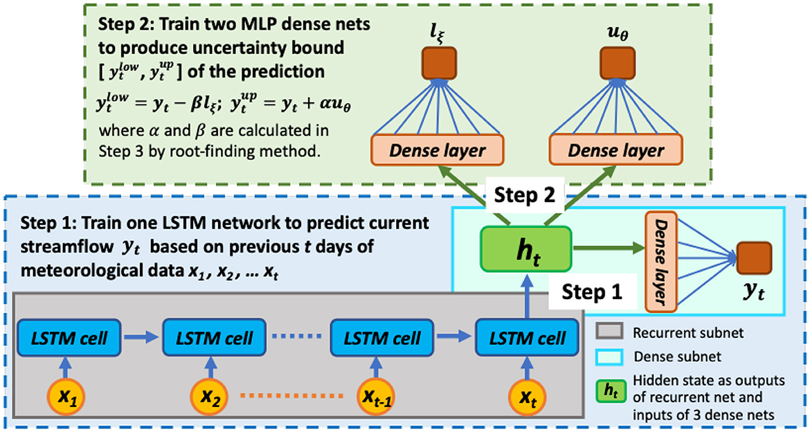
Figure 1. The workflow of the PI3NN-LSTM method where a LSTM network is trained for prediction and two MLP networks are trained for UQ.
To enable the application of PI3NN for the complex LSTM networks and meanwhile maintain the method's simplicity and computational efficiency, we propose the following network decomposition strategy. First, we decompose the LSTM model into two subnets: a recurrent net and a subsequent MLP dense net. The recurrent subnet learns input features and their temporal information in the period of look-back window t, and saves this information in the hidden state variables ht, i.e., [x1, x2, ....xt] → ht. Subsequently, the dense subnet learns the input-output relationship from ht to yt, i.e., ht→yt. After the entire LSTM model is trained, the vector ht will save all the information of the meteorological input sequences. Then, we can use ht as a new set of inputs for the MLP network to predict the current streamflow of yt and quantify its predictive uncertainty, without considering the recurrent subnet anymore. In this way, we successfully transform the problem of quantifying predictive uncertainty on the complex LSTM models into the UQ problem on the simple MLP models, which greatly simplifies the task.
To summarize, we perform the following three steps to integrate PI3NN into LSTM for time-series prediction and predictive uncertainty quantification (Figure 1) :
• Step 1. Train a LSTM model to predict yt from multivariate input sequences of [x1, x2, ....xt] in a standard way;
• Step 2. Perform the network decomposition and extract values of the hidden state variables ht as inputs and calculate the difference between the LSTM model prediction and observation on yt as outputs to train two MLP networks for estimating the PI;
• Step 3. Determine the PI of yt precisely by computing the coefficients of α and β via the root-finding method.
In comparison to the three steps in Section 2.1, PI3NN-LSTM has the following similarities and novelties. Step 1 is similar. Both train a ML model fω(x), either a MLP model or a LSTM model, in a standard way for deterministic prediction. Step 2 is novel here. The PI3NN-LSTM method takes the network decomposition strategy and uses the hidden state variables ht as the inputs instead of the original model inputs for the calculation of the PIs, where the size of ht is equal to the number of LSTM cells. In this way, PI3NN-LSTM can use two MLP networks uθ and lξ for the UQ of the LSTM model. Additionally, these two MLP networks can have simple structures because their inputs of ht usually have simpler structures than the original LSTM inputs of multiple sequences [x1, x2, ....xt]. Also, the MLP networks can be fully connected or use dropout depending on the problem and data size, but dropout is not necessary for our algorithm. Step 3 is the same as in Section 2.1. By employing the techniques in Section 2.2, the PI3NN-LSTM method can also examine the OOD samples in the time-series simulation and characterize the possible data/domain shift to avoid overconfident predictions. The strategy of network decomposition is the key here to enable the simple and computationally efficient calculation of the PIs for complex LSTM models. And this strategy can be generally applied to other deep learning networks. For example, we can decompose a convolutional neural network (CNN) model into a convolutional net and a MLP dense net, and decompose a graph neural network (GNN) model into a graph net and a MLP dense net. The recurrent net, convolutional net, and graph net in the LSTM, CNN, and GNN model, respectively, perform like an encoder which extracts temporal, spatial, and graphical information into a hidden/latent variable. Then, we implement PI3NN on these hidden variables to simplify the UQ task into the MLP problem to enable its general application.
PI3NN-LSTM uses three networks to quantify the prediction uncertainty affected by data noise and under new conditions. Its OOD identification capability describes what the ML model does not know outside the training regime to mitigate overconfidence, this description somehow addresses the model structural uncertainty. Some methods such as deep ensembles (Lakshminarayanan et al., 2017) used ensemble sampling to quantify prediction uncertainty and address the model structural uncertainty. Our method can be applied to different model structures to further consider the influence of model structural uncertainty on the prediction.
3. Application of PI3NN to two diverse watersheds
We apply the PI3NN-LSTM method for daily streamflow prediction and UQ from meteorological observations in the snow-dominant East River Watershed (ERW) and the rain-driven Walker Branch Watershed (WBW) in the western and southeastern US, respectively. The two watersheds are distinctly different in their climatological patterns and hydrological dynamics, thus these applications enable us to investigate whether PI3NN-LSTM is able to provide consistently good predictions under different conditions.
3.1. Snow-dominant East River Watershed (ERW)
ERW is located in Colorado, US and it contains several headwater catchments in the Upper Colorado River basin. The watershed is about 300 km2 and has an average elevation of 3266 m above mean sea level, with 1420 m of topographic relief and pronounced gradients in hydrology, vegetation, geology, and weather. The area is defined as having a continental, subarctic climate with long, cold winters and short, cool summers. The watershed has a mean annual temperature of 0C, with average minimum and maximum temperatures of -9.2C and 9.8C, respectively; winter and growing seasons are distinct and greatly influence hydrology. Annual average precipitation is approximately 1200 mm/yr and is mostly snow. River discharge is driven by snowmelt in late spring and early summer and by monsoonal-pattern rainfall in summer (Hubbard et al., 2018).
We consider data from two gauged stations, Quigley and Rock creek, both of which are headwater catchments with areas of 2.33 km2 and 3.24 km2, respectively. Each catchment includes four sequences of data: three input sequences of daily precipitation, maximum air temperature, and minimum air temperature, and one output sequence of daily streamflow. Quigley catchment has about 2 years of meteorological and streamflow observations from 09/01/2014 to 10/13/2016 with 774 daily measurements. Rock creek catchment has about 3 years of observations from 08/31/2014 to 10/04/2017 with 1131 daily measurements. In the LSTM simulation, we reserve the last year as the unseen test data for prediction performance evaluation and use the remaining data for training. These two catchments have short records, which is a deliberate choice. As a new development of the PI3NN-LSTM method and the first application to streamflow prediction, we want to first use a relatively small dataset, where the trained model could suffer from significant predictive uncertainty due to limited available data, for detailed analyses of performance in both InD and OOD situations. And then in the second case study of WBW, we work with a longer record of data for further investigation and demonstration.
3.2. Rain-driven Walker Branch Watershed (WBW)
WBW is located in East Tennessee, US, and is part of the Clinch River which ultimately drains into the Mississippi River (Curlin and Nelson, 1968; Griffiths and Mulholland, 2021). WBW includes the West Fork and East Fork catchments, which are 0.384 km2 and 0.591 km2 in size, respectively. WBW has an average annual rainfall of 1350 mm and a mean annual temperature of 14.5C, which is consistent with a humid southern Appalachian region climate. The watershed elevation ranges from 265 m to 351 m above mean sea level. Rain is the primary precipitation type in this region. Streamflow in both the West Fork and East Fork catchments is perennial and is fed by multiple springs (Johnson, 1989). We use data from the East Fork catchment in this study. The data consist of seven input sequences, including daily precipitation, maximum and minimum air temperature, maximum and minimum relative humidity, and maximum and minimum soil temperature, and one output sequence of daily streamflow. We have 14 years of observations from 01/01/1993 to 12/31/2006 with 5113 daily measurements. Given this long record of data, we reserve the last 4 years (2003–2006) as unseen test data for prediction performance evaluation and use the first 10 years of data for training.
3.3. Implementation and performance evaluation metrics
For both watersheds, we use LSTM networks for streamflow prediction and PI3NN method to calculate the 90% prediction interval for uncertainty evaluation. In the networks training stage, we use 20% of the training data as validation set to tune the network structure and the learning hyperparameters through the random search method. We then choose the model structure and hyperparameters that give the best performance, i.e., the smallest MSE, in simulating the validate data as the final model. Specifically, for the LSTM network, we consider one or two layers with the number of nodes in the set of [32, 64, 128, 256] and the look-back window size in the set of [30, 45, 60, 75, 90, 120]. For the two MLP networks used for UQ, we consider one or two layers with the number of nodes in the set of [10, 20, 30, 40, 50]. For all the three networks, we use Adam optimizer with consideration of the learning rate between 0.001 and 0.01 with an increment of 0.001. The final network structures and hyperparameters are summarized in the following Table 1. Note that these hyperparameters are tuned based on validation data performance. The complexity of a NN's structure depends on several factors including the input-output relationship extracted from the data and data size. A shorter record of data does not necessarily require a simpler network structure than the longer record as long as the network complexity produces a good performance and does not suffer from overfitting. Moreover, these hyperparameters are standard for NNs. Our PI3NN method does not introduce extra hyperparameters which saves the effort of tedious tuning and more importantly promises stable prediction performance. Additionally, the MLP networks used by PI3NN usually have a simple structure which enables a data- and computationally-efficient training and UQ.
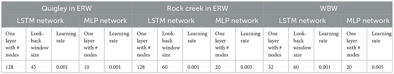
Table 1. The network model structures and their learning parameters used in streamflow prediction and UQ for both watersheds ERW and WBW.
We then use the trained models to predict the streamflow and quantify the predictive uncertainty in the test period. We use the Nash-Sutcliffe-Efficiency (NSE) to assess model prediction accuracy, and use the Prediction Interval Coverage Probability (PICP) and Prediction Interval Width (PIW) jointly to evaluate the quality of the UQ. NSE is an established measure used in the hydrological modeling to evaluate streamflow simulation accuracy based on the following equation:
where N is the total number of samples in evaluation, represents predictions, and are the observations and mean observations, respectively. The range of the NSE is (-inf, 1], where a value of 1 means a perfect simulation, a NSE of 0 means the simulation is as good as the mean of the observations, and everything below 0 means the simulation is worse compared to using the observed mean as a prediction. According to N. Moriasi et al. (2007), a NSE value greater than 0.50 is considered satisfactory, greater than 0.65 is considered good, and greater than 0.75 is very good.
PICP is defined as the ratio of samples that fall within their respective PIs. For example, for a sample set , we use ki to indicate whether the sample yi is enclosed in its PI [L, U], i.e.,
Then, the total number of samples within upper and lower bounds is counted as:
Consequently, the PICP is calculated as:
For each prediction data, the PIW is calculated as
A high-quality uncertainty estimate should produce a PICP value close to its desired confidence level with a small PIW for InD data to demonstrate its accuracy and precision, and should be able to quantify uncertainty with a large PIW for the OOD data to avoid overconfident predictions.
4. Results and discussion
In this section, we evaluate the PI3NN-LSTM model's prediction performance. We assess the prediction accuracy using the NSE score and by comparing the observed and simulated hydrographs. We investigate the UQ capability based on three aspects: the quality of the PI, the robustness, and data-, computational-efficiency of the method, and its capability in identification of OOD samples. In the following, we first analyze the results from the two snow-dominant catchments in ERW with short records of streamflow observations and then move to rain-driven WBW with a relatively long record of data. We discuss the results in ERW in detail and briefly summarize the findings in WBW as an extensive demonstration.
4.1. Streamflow prediction in snow-dominant ERW
Figure 2 depicts the 2 years of data in Quigley catchment where the top panel shows the 1 year of training data and the bottom panel shows the following year of unseen test data. This figure describes the rainfall-runoff dynamics of a typical snow-dominant watershed. Streamflow peaks in the spring/early summer and precipitation is highest in the winter from snowfall. The time lag between precipitation and streamflow can be explained by snow accumulation in the winter months and subsequent snow melt in spring. The LSTM network is able to successfully simulate this rainfall-runoff relationship and its memory effects by producing the predicted streamflow close to the observations based only on the precipitation and temperature inputs. The NSE value for the training data is 0.94 and for the test data is 0.87, suggesting a high prediction accuracy. Moreover, a close look at the figure shows that in both training and test periods, the predicted hydrograph fits the general trends of the observation pretty well with a close peak flow timing and similar rising and falling limb shapes.
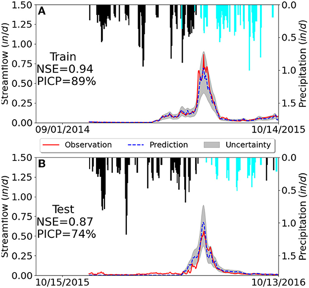
Figure 2. Predicted (dashed blue line) and observed streamflow (solid red line) in the snow-dominant Quigley catchment where the gray area quantifies the 90% predictive interval. Daily precipitation is plotted upside down on the top associated with the right y-axis, where snow (temperature below 0°C and in snow-water equivalents) is highlighted in black. Subfigures (A, B) illustrate the results from training and test data sets, respectively.
In Figure 2, we can also see that PI3NN accurately quantifies the predictive uncertainty where the PICP value of 89% in training data is close to its desired confidence level of 90%. Furthermore, the uncertainty bound covers the observations with a narrow width, demonstrating an informative UQ. Figure 3 summarizes the PIW for the training and test data using boxplots. It can be seen that the largest PIW in the training set of Quigley catchment is about 0.5 in/d, which occurred when simulating peak flow where the LSTM model shows a relatively large error (Figure 2A). For the data points with accurate streamflow simulation, PI3NN produces a relatively narrow uncertainty bound with a small interval width, presenting high confidence in line with the high accuracy. The similar PIW of the training and test data for Quigley shown in Figure 3 indicates that no OOD samples have been detected in this catchment and that the LSTM model predictions in the test period can be trusted. Indeed, we observe a high prediction accuracy of the test data as validated by the observations in Figure 2B and its PICP value suggests that about 74% of the test data are enclosed in the uncertainty bound. Note that, we do not expect the 90% PI to enclose the exact 90% of the test data. PI3NN is guaranteed to produce the exact coverage for the training data because of its root-finding strategy. But for the unknown test data, a different feature from the training set would cause a different prediction performance and predictive uncertainty coverage.
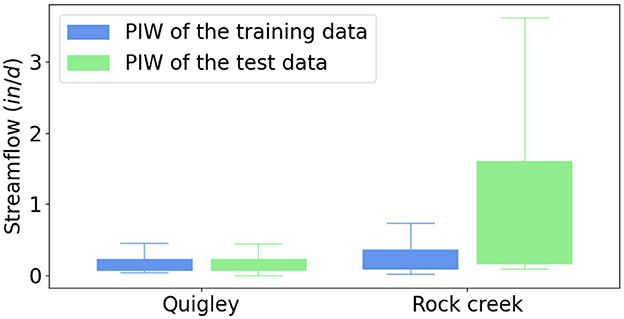
Figure 3. Prediction interval width (PIW) of the training and test data for the Quigley and Rock creek catchments in ERW. The similar PIW between the training and test data in Quigley indicates that the prediction for the test period can be trusted. In contrast, the largely different PIW between the training and test data in Rock creek suggests that its test period encounters some new climates that have not been seen before in training and the ML predictions may not be trusted.
Figure 4 illustrates 3 years of data in Rock creek catchment where the top panel shows 2 years of training data and the bottom panel shows 1 year of test data. The test period of 2017 is a wet, cold year with unusually high precipitation (snow accumulation) in winter. Rock creek is a small headwater catchment and its streamflow is rather sensitive to the meteorological forcings, so the high precipitation in winter results in a correspondingly large peak flow in summer from snow melt, showing a data/domain shift relative to the training period of 2015-2016. In this case study, we want to investigate the LSTM model's capability in predicting the OOD samples caused by the new climate condition and more importantly to examine whether PI3NN can identify the data/domain shift and produce a large uncertainty by showing low confidence based on these anomalies.
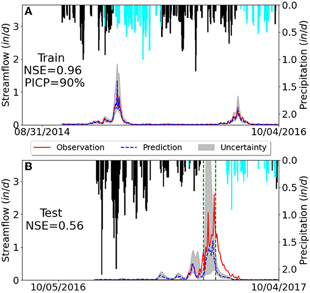
Figure 4. Predicted (dashed blue line) and observed streamflow (solid red line) in the snow-dominant Rock creek catchment where the gray area quantifies the predictive uncertainty. Corresponding daily precipitation is plotted upside down where snow (temperature below 0°C) is highlighted in black. Subfigures (A, B) illustrate the results from training and test data sets, respectively.
Figure 3 clearly shows that the test data in Rock creek have a much larger PIW compared to the training set. This large difference in the uncertainty intervals indicates that the test samples contain some features that have not been learned before and the predictions on some of these samples cannot be trusted. Taking a close look at the hydrograph in the test period of Figure 4B, we observe that the uncertainty bound in the peak flow regions between the two green dashed lines are remarkably high, and indeed this highly uncertain region has a larger prediction error where the model-predicted streamflow deviates from the observations the most. This underestimation of peak flow is understandable because the ML model only saw relatively low precipitation in the training period. Importantly, PI3NN is able to identify this underestimation by giving it a high uncertainty and a low confidence, suggesting that the model predictions on these data points should not be trusted, although the model has a good prediction performance in training. This error-consistent uncertainty information is very useful in real-world applications where the groundtruthed data are unavailable. The calculated uncertainty can serve as a prediction error quantifier (which is usually calculated as the difference between the predictions and the observations) to indicate the ML prediction's credibility to avoid overconfident predictions.
Note that, PI3NN identifies OOD samples based on their input features. If the data points are an anomaly in input space (e.g., extreme climates) then PI3NN can identify them and produce a high uncertainty in the output predictions (e.g., streamflow). However, if some data points have input features similar to the training set, although their predictions are poor, PI3NN or any other UQ methods cannot assign them large predictive uncertainties. In Rock creek catchment, the input space of the two MLP dense networks used for calculating the PIs are the 128 hidden state variables (ht). We project the training and test samples of ht from their original 128-dimensional space to the 2-dimensional space using principal component analysis for visualization. Figure 5 indicates that there are 21 test data, at the upper right corner highlighted in green, relatively far away from other points and can be identified as OOD samples. We find that these 21 input data result in the streamflow predictions between the two green dashed lines in Figure 4B where PI3NN gives them large predictive uncertainties. This analysis explains the OOD identification capability of PI3NN. It demonstrates that if new climates make the trained ML model fail to accurately predict streamflow, PI3NN can correctly identify these new conditions and reasonably reflect their influence on streamflow prediction by producing a large uncertainty.
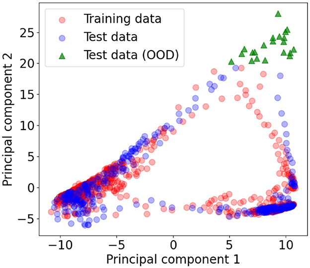
Figure 5. Projecting the training and test data of the input hidden state variable (ht) from its original 128 dimensions to the 2-dimensional space using principal component analysis for visualization. The 21 points (highlighted in green triangles) of the test data are identified as OOD samples, which suggests that their predicted streamflow cannot be trusted. These streamflow predictions are located between the two green dashed lines in Figure 4B which indeed shows poor prediction accuracy.
In the above analysis of ERW data, we demonstrate the PI3NN-LSTM's prediction accuracy, predictive uncertainty quality, and OOD identification capability. In the following, we discuss its robustness and efficiency. First of all, PI3NN is computationally efficient. It quantifies predictive uncertainty using three NNs' training where the first network is the standard LSTM for mean prediction, and the other two are MLP networks to calculate the prediction interval. In both catchments, we use a single-layer MLP network whose training only takes 10–20 s and the computational cost of the following root-finding step is negligible (less than 1 s). Also, for a different confidence level, PI3NN just needs to perform the root-finding step to determine the corresponding uncertainty bounds without further network training, and the calculated intervals are well-calibrated and consistent with the confidence level. As illustrated in Figure 6 where both the 90% and 95% prediction intervals are plotted, the 95% PI encloses 95% of training data (PICP=95%) and its width is wider than the 90% interval. Note that, it only takes about 20 seconds of PI3NN to accurately calculate these predictive uncertainties for a range of confidence levels after the standard LSTM model simulation. Moreover, PI3NN is data efficient. Attributed to the LSTM network decomposition strategy (Section 2.3), we are able to use rather simple MLP networks to estimate the uncertainty bound; and the simple network structures enable a small number of training data for an accurate learning. Here, by using 1 year of training data in Quigley and 2 years of training data in Rock creek, we are able to reasonably quantify the uncertainty and correctly identify the OOD samples.

Figure 6. Streamflow observations and predictions for different confidence levels (γ) in the Quigley catchment. The 95% PI (γ=0.95) encloses 95% of the observations (PCIP=95%) and the 95% interval is wider than the 90% interval (γ=0.9) showing accuracy of the PI3NN method. Subfigures (A, B) illustrate the results from training and test data sets, respectively.
Additionally, PI3NN is assumption-free. It does not involve a Gaussian assumption of the data noise, which makes it practically applicable to hydrological observations. And it is also able to generate an asymmetric uncertainty bound to precisely quantify the desired confidence level with a narrow width. Furthermore, PI3NN does not introduce extra hyperparameters allowing for stable performance. The only non-standard parameter that needs to be specified in PI3NN is the constant c in initializing the output layer bias when using its OOD identification capability. In Figure 7, we demonstrate that as long as c is specified with a large positive value, PI3NN is able to detect the OOD samples by showing a larger PIW comparing to the training set. The exact value of c does not matter much and would barely affect the UQ quality. As we can see, with a different c, the PIWs of the training data are similar to each other and the specification of c does not affect the uncertainty coverage. For unseen test data, if OOD samples exist, a large c will lead to a large PIW enabling the identification of data/domain shift, although the larger the c value is, the more obvious the identification.
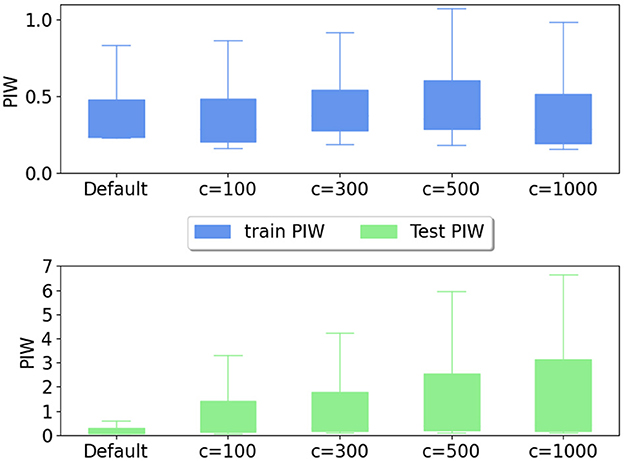
Figure 7. PIW of the training and test data for different output layer bias initialization in training the two interval networks for the Rock creek catchment. A larger c value initializes the bias to a larger value and the default c value usually draws a sample from a standard Gaussian distribution. Different c values do not affect training and any large c values here can identify the OOD samples with large PIWs, which indicates the reliability of PI3NN.
PI3NN is also a robust uncertainty estimate which produces error-consistent confidence. Figure 8 visualizes the relationship between absolute prediction errors and the PIW for both the training and test data sets in the Rock creek catchment. A clear monotonic trend is observed where the PIW increases as the increase of the errors, exhibiting decreasing confidence with the degradation of the prediction accuracy. Moreover, the identified OOD samples which cannot be accurately predicted by the ML model show a large PIW and a large error at the upper right corner of Figure 8B. This error-consistent UQ property enables us to confidently use PI3NN as a ML model trustworthiness quantifier to diagnose when the model predictions can be trusted and when the models may fail for the new conditions.
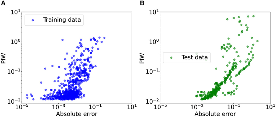
Figure 8. Scatter plots of absolute prediction errors VS. the PIW for both the training (A) and test (B) data sets in Rock creek catchment. The prediction interval shows error-consistent uncertainty where high uncertainties (i.e., large PIWs) correspond to large errors.
4.2. Streamflow prediction in rain-driven WBW
In this section, we summarize the results from applying the PI3NN-LSTM model for streamflow prediction in rain-driven WBW. Figure 9 depicts 10 years of training (top) and 4 years of test data (bottom) in the East Fork of WBW. In comparison to Figures 2, 4 that depict snow-dominant hydrological dynamics, this rain-driven watershed has many fewer snow days and shows a faster runoff response after a precipitation event. The training and test periods have similar magnitudes of precipitation on both annual and event scales. In fact, we find that all the meteorological forcing inputs are of a similar magnitude in the training and test sets. PI3NN did not identify OOD samples in this dataset.

Figure 9. Predicted (dashed blue line) and observed streamflow (solid red line) in the East Fork of rain-driven WBW. Also shown in green lines are LSTM predictions using weighted mean squared errors as the loss function. Corresponding daily precipitation is plotted upside down on the top associated with the right y-axis, where snow (temperature below 0°C) is highlighted in black. (A) Training data of 1993–2002. (B) Test data of 2003–2006.
Figure 9 indicates that the LSTM network is able to simulate the streamflow reasonably well by showing a good fit to the observations. The overall NSE is 0.65 for the training data and 0.6 for the test data. Figure 10 plots each test year individually where both the predictive values and the 90% PI are depicted. Different years demonstrate different prediction accuracies, e.g., the NSE in 2005 is up to 0.78 while the subsequent year (2006) has a relatively low NSE of 0.50. In all the four test years, the LSTM model appears to underpredict peak flows, e.g., the observed peak flow is 617 L/s in 2003, but the predicted peak flow is 194 L/s; the observed peak flow is 274 L/s in 2004, and the predicted peak flow is 128 L/s. In this rain-driven watershed, peak flow happens during storms. It seems that the LSTM model has difficulties accurately predicting the magnitude of these event-triggered streamflows and the underprediction in peak flows results in the relatively low NSEs in most test years. Looking at the training period in Figure 9A, it seems that even for the training data, LSTM has some underpredictions of peak flows. To explore the possible reasons for the underprediction, we designed another numerical experiment where we used weighted mean squared errors (wMSE) as the loss function in training with the weight proportional to the streamflow observations. Results indicate that the wMSE loss did not improve the underprediction of peak flows and even made the fitting worse compared to the standard MSE loss by penalizing the fit of low flow. The overall NSE is 0.55 of wMSE compared to 0.65 of the MSE in training and the NSE is 0.43 of wMSE compared to 0.6 of MSE in testing. We think one possible reason is that these peak flows are erratic events which have relatively small observations compared to other streamflow data. ML models are data driven, and the small sets of data can deteriorate LSTM's capability in learning the underlying mechanism causing the high peak flows. Future investigations are needed to examine this possibility.
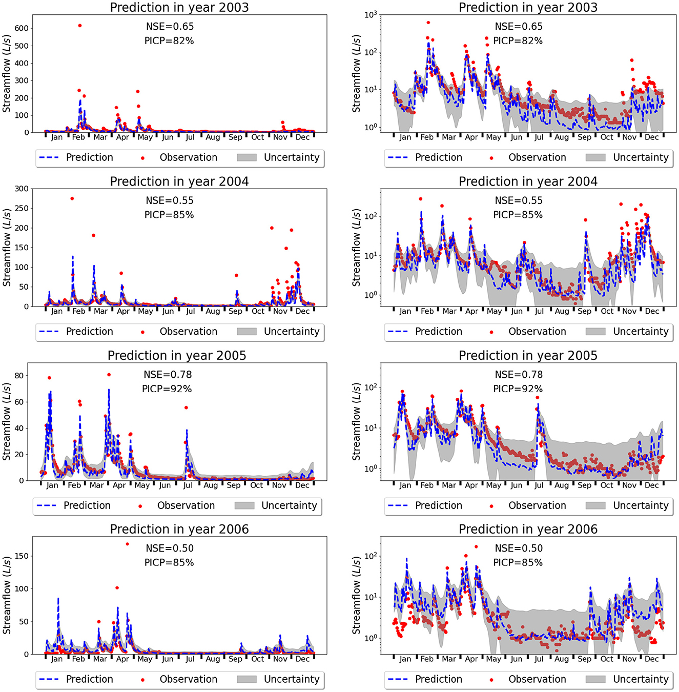
Figure 10. Predicted (dashed blue line) and observed streamflow (red dots) in the East Fork of rain-driven WBW where the gray area quantifies the 90% prediction interval. Figures in the left column have a linear scale on the y-axes to show the underprediction of peak flows while figures on the right have a logarithmic scale on the y-axes to show the accurate prediction and predictive uncertainty of base flows. Note that the y-axis range on each figure is different.
On the other hand, the peak flow timing in the test years is accurately predicted. For example, peak flow in 2003 was observed on the 47th day of the year and was predicted to occur on the 48th day. Peak flow was observed on the 37th day of 2004 and was predicted to happen on the 38th day. Both the observed and predicted peak flow happened on the 92nd day of 2005. Additionally, the LSTM model does a good job at predicting base flows. Zooming into the base flow regions by plotting the streamflow in logarithmic scale in Figure 10, we can see that the predicted base flows are close to the observations with a high consistency. Additionally, the predictive uncertainty in the test period can be precisely quantified by PI3NN, where the calculated PICP is close to the desired value of 90% and most of the observed base flows are encompassed by the prediction intervals. PI3NN does not assume a Gaussian distribution for the data so it can produce an asymmetric uncertainty bound to precisely cover the observations. For example, in August-October of 2003 where the model underpredicts streamflow, PI3NN produces a higher upper bound of the prediction interval to cover the observations. Note that the predictive uncertainty associates with the prediction; if the predicted value greatly deviates from the observation and OOD samples are not detected, then we cannot expect the uncertainty bound encloses the observations. However, it is interesting to see that although the prediction accuracy is not very high for some years, e.g., the NSE is 0.5 in 2006, the prediction interval can cover the desired number of observations nicely with the PICP of 85%.
WBW has a complex geomorphological structure and interconnected hydrological processes (Griffiths and Mulholland, 2021). Many topographical, geological, soil, and ecological factors affect streamflow dynamics. However, in this model, we only consider a few meteorological variables as the inputs to simulate streamflow, which may result in poor predictions due to the limited input data and some missing information on important cause-effects. It is usually the case that the data, including the number of input variables and the number of observations, are too few to enable the ML model to accurately capture the underlying mechanisms of complex hydrological dynamics in watersheds. UQ cannot address the lack of data and it is not a replacement for data acquisition, but instead, the calculated large uncertainty can guide data collection to reduce the uncertainty. Additionally, it is promising to see here that the reasonably quantified uncertainty from PI3NN can encompass the desired number of observations despite the relatively poor fit.
5. Conclusions and future work
In this study, we further develop our PI3NN method to enable the quantification of predictive uncertainty of various deep learning networks and integrate the method with the LSTM network for streamflow prediction. Application of the PI3NN-LSTM approach to both snow-dominant and rain-driven watersheds demonstrates its prediction accuracy, high-quality predictive uncertainty quantification, and the method's robustness, and data- and computational-efficiency. For the test data which have similar features as the training data, PI3NN can precisely quantify the predictive uncertainty with the desired confidence level; and for the OOD samples where the LSTM model fails to make accurate predictions, PI3NN can produce a reasonably large uncertainty indicating that the results are not trustworthy. Additionally, PI3NN produces error-consistent uncertainties where the prediction interval width increases as the prediction accuracy decreases. Therefore, when we apply the ML model to predict streamflow under future climate and at ungauged catchments where no groundtruthed data are available, the uncertainty quantifies the model predictions' trustworthiness, indicating whether the results should be trusted or further investigation needs to be conducted. PI3NN is computationally efficient, robust in performance, and generalizable to multiple data with no distributional assumptions. Attributed to the network decomposition strategy proposed in this work, PI3NN now can be broadly applied to various networks including convolutional networks, graph networks, recurrent networks, and the combined model structures of these networks, for trustworthy hydrological predictions.
Although data are a key to improve ML model predictability, UQ is significantly important for quantifying the influence of data quality and the trustworthiness of the predictions under the changing climate and environmental conditions. Additionally, we can use UQ to guide the data collection in the large-uncertainty regime and to examine the model deficiency for further model development and improvement. In the future, we will apply PI3NN for streamflow prediction in multiple watersheds across the US and integrate it with different ML models for a variety of hydrological applications.
Author's note
This manuscript has been authored by UT-Battelle LLC, under contract DE-AC05-00OR22725 with the US Department of Energy (DOE). The US government retains and the publisher, by accepting the article for publication, acknowledges that the US government retains a nonexclusive, paid-up, irrevocable, worldwide license to publish or reproduce the published form of this manuscript, or allow others to do so, for US government purposes. DOE will provide public access to these results of federally sponsored research in accordance with the DOE Public Access Plan (http://energy.gov/downloads/doe-public-access-plan).
Data availability statement
Publicly available datasets were analyzed in this study. This data can be found at the following links: For East River Watershed: https://github.com/liusiyan/UQnet/tree/PI3NN_LSTM_dev/datasets/Timeseries/StreamflowData. For Walker Branch Watershed: https://walkerbranch.ornl.gov. The PI3NN code is available at https://github.com/liusiyan/PI3NN.
Author contributions
SL implemented the numerical experiments, summarized the results, and prepared the figures. DL developed the algorithms, planned the research, plotted the figures, interpreted the results, and drafted the manuscript. SP, NG, and EP processed the data and interpreted the results. All the authors contributed to the manuscript writing. All authors contributed to the article and approved the submitted version.
Funding
This research was supported by the Artificial Intelligence Initiative as part of the Laboratory Directed Research and Development Program of Oak Ridge National Laboratory, managed by UT-Battelle, LLC, for the US DOE under contract DE-AC05-00OR22725. It is also sponsored by the ExaSheds project and the Watershed Dynamics and Evolution (WaDE) Science Focus Area project funded by the US DOE, Office of Biological and Environmental Research. We thank Pat Mulholland for collecting and maintaining the WBW streamflow data for many years.
Conflict of interest
The authors declare that the research was conducted in the absence of any commercial or financial relationships that could be construed as a potential conflict of interest.
Publisher's note
All claims expressed in this article are solely those of the authors and do not necessarily represent those of their affiliated organizations, or those of the publisher, the editors and the reviewers. Any product that may be evaluated in this article, or claim that may be made by its manufacturer, is not guaranteed or endorsed by the publisher.
References
Abbaszadeh Shahri, A., Shan, C., and Larsson, S. (2022). A novel approach to uncertainty quantification in groundwater table modeling by automated predictive deep learning. Natural Resour. Res. 31, 1351–1373. doi: 10.1007/s11053-022-10051-w
Althoff, D., Rodrigues, L. N., and Bazame, H. C. (2021). Uncertainty quantification for hydrological models based on neural networks: the dropout ensemble. Stochastic Environ. Res. Risk Assessm. 35, 1051–1067. doi: 10.1007/s00477-021-01980-8
Amini, A., Schwarting, W., Soleimany, A., and Rus, D. (2020). “Deep evidential regression,” in Proceedings of the 34th International Conference on Neural Information Processing Systems (Vancouver, BC: Curran Associates Inc), 1–11. doi: 10.5555/3495724.3496975
Clark, M., Wilby, R., and Gutmann, E. E. A. (2016). Characterizing uncertainty of the hydrologic impacts of climate change. Curr. Clim. Change Rep. 2, 55–64. doi: 10.1007/s40641-016-0034-x
Curlin, J. W., and Nelson, D. J. (1968). Walker Branch Watershed Project: Objectives, Facilities, and Ecological Characteristics. ORNL/TM-2271. Oak Ridge National Laboratory, Oak Ridge, Tennessee, United States.
Fang, K., Kifer, D., Lawson, K., and Shen, C. (2020). Evaluating the potential and challenges of an uncertainty quantification method for long short-term memory models for soil moisture predictions. Water Resour. Res. 56, 12. doi: 10.1029/2020WR028095
Feng, D., Fang, K., and Shen, C. (2020). Enhancing streamflow forecast and extracting insights using long-short term memory networks with data integration at continental scales. Water Resour. Res. 56, e2019WR026793. doi: 10.1029/2019WR026793
Gal, Y., and Ghahramani, Z. (2016a). “Dropout as a bayesian approximation: representing model uncertainty in deep learning,” in Proceedings of The 33rd International Conference on Machine Learning, volume 48 of em Proceedings of Machine Learning Research, eds M. F. Balcan and K. Q. Weinberger (New York, NY: PMLR), 1050–1059.
Gal, Y., and Ghahramani, Z. (2016b). “A theoretically grounded application of dropout in recurrent neural networks,” in Proceedings of the 30th International Conference on Neural Information Processing Systems (Barcelona: Curran Associates), 1027–1035. doi: 10.5555/3157096.3157211
Gan, Y., Duan, Q., Gong, W., Tong, C., Sun, Y., Chu, W., et al. (2014). A comprehensive evaluation of various sensitivity analysis methods: a case study with a hydrological model. Environ. Model. Software 51, 269–285. doi: 10.1016/j.envsoft.2013.09.031
Griffiths, N. A., and Mulholland, P. J. (2021). Long-term hydrological, biogeochemical, and climatological data from walker branch watershed, east tennessee, usa. Hydrol Process. 35, e14110. doi: 10.1002/hyp.14110
Hochreiter, S., and Schmidhuber, J. (1997). Long short-term memory. Neural Comput. 9, 1735–1780. doi: 10.1162/neco.1997.9.8.1735
Hubbard, S. S., Williams, K. H., Agarwal, D., Banfield, J., Beller, H., Bouskill, N., et al. (2018). The east river, colorado, watershed: a mountainous community testbed for improving predictive understanding of multiscale hydrological? biogeochemical dynamics. Vadose Zone J. 17, 1–25. doi: 10.2136/vzj2018.03.0061
Klotz, D., Kratzert, F., Gauch, M., Keefe Sampson, A., Brandstetter, J., Klambauer, G., et al. (2022). Uncertainty estimation with deep learning for rainfall-runoff modeling. Hydrol. Earth Syst. Sci. 26, 1673–1693. doi: 10.5194/hess-26-1673-2022
Konapala, G., Kao, S.-C., Painter, S. L., and Lu, D. (2020). Machine learning assisted hybrid models can improve streamflow simulation in diverse catchments across the conterminous us. Environ. Res. Lett. 15, 104022. doi: 10.1088/1748-9326/aba927
Kratzert, F., Klotz, D., Brenner, C., Schulz, K., and Herrnegger, M. (2018). Rainfall-runoff modelling using long short-term memory (lstm) networks. Hydrol. Earth Syst. Sci. 22, 6005–6022. doi: 10.5194/hess-22-6005-2018
Kratzert, F., Klotz, D., Herrnegger, M., Sampson, A. K., Hochreiter, S., and Nearing, G. S. (2019). Toward improved predictions in ungauged basins: Exploiting the power of machine learning. Water Resour. Res. 55, 11344–11354. doi: 10.1029/2019WR026065
Lakshminarayanan, B., Pritzel, A., and Blundell, C. (2017). “Simple and scalable predictive uncertainty estimation using deep ensembles,” in Proceedings of the 31st International Conference on Neural Information Processing Systems, NIPS'17 (Red Hook, NY: Curran Associates Inc.), 6405–6416.
Liu, J. Z., Lin, Z., Padhy, A., Tran, D., Bedrax-Weiss, T., and Lakshminarayanan, B. (2020). “Simple and principled uncertainty estimation with deterministic deep learning via distance awareness,” in Proceedings of the 34th International Conference on Neural Information Processing Systems (Vancouver, BC: Curran Associates). doi: 10.5555/3495724.3496353
Liu, S., Zhang, P., Lu, D., and Zhang, G. (2022). “PI3NN: out-of-distribution-aware prediction intervals from three neural networks,” in International Conference on Learning Representations (Virtual).
Loquercio, A., Segu, M., and Scaramuzza, D. (2020). A general framework for uncertainty estimation in deep learning. IEEE Rob. Autom. Lett. 5, 3153–3160. doi: 10.1109/LRA.2020.2974682
Lu, D., Konapala, G., Painter, S. L., Kao, S.-C., and Gangrade, S. (2021). Streamflow simulation in data-scarce basins using bayesian and physics-informed machine learning models. J. Hydrometeorol. 22, 1421–1438. doi: 10.1175/JHM-D-20-0082.1
Lu, D., Liu, S., and Ricciuto, D. (2019). “An efficient bayesian method for advancing the application of deep learning in earth science,” in 2019 International Conference on Data Mining Workshops (ICDMW) (Beijing: IEEE), 270–278.
Lu, D., Ye, M., and Hill, M. C. (2012). Analysis of regression confidence intervals and bayesian credible intervals for uncertainty quantification. Water Resour. Res. 48, WR011289. doi: 10.1029/2011WR011289
Moriasi, D. N., Arnold, J. G., Van Liew, M. W., Bingner, R. L., Harmel, R. D., and Veith, T. L. (2007). Model evaluation guidelines for systematic quantification of accuracy in watershed simulations. Trans. ASABE 50, 885–900. doi: 10.13031/2013.23153
Pearce, T., Leibfried, F., and Brintrup, A. (2020). “Uncertainty in neural networks: approximately bayesian ensembling,” in Proceedings of the Twenty Third International Conference on Artificial Intelligence and Statistics, volume 108 of Proceedings of Machine Learning Research, eds S. Chiappa and R. Calandra (Palermo: PMLR), 234–244.
Pearce, T., Brintrup, A., Zaki, M., and Neely, A. (2018). “High-quality prediction intervals for deep learning: a distribution-free, ensembled approach,” in Proceedings of the 35th International Conference on Machine Learning, volume 80 of Proceedings of Machine Learning Research, eds J. Dy and A. Krause (Stockholm: PMLR), 4075–4084.
Pechlivanidis, I. G., Jackson, B., McIntyre, N., and Wheater, H. S. (2011). Catchment scale hydrological modelling: a review of model types, calibration approaches and uncertainty analysis methods in the context of recent developments in technology and applications. Global Nest J. 13, 193–214. doi: 10.30955/gnj.000778
Rasouli, K., Hsieh, W. W., and Cannon, A. J. (2012). Daily streamflow forecasting by machine learning methods with weather and climate inputs. J. Hydrol. 414–415, 284–293. doi: 10.1016/j.jhydrol.2011.10.039
Salem, S. T., Langseth, H., and Ramamipiaro, H. (2020). “Prediction intervals: Split normal mixture from quality-driven deep ensembles,” in Proceedings of the 36th Conference on Uncertainty in Artificial Intelligence (UAI), eds J. Peter and D. Sontag (PMLR), 1179–1187. Available online at: http://proceedings.mlr.press/v124/saleh-salem20a/saleh-salem20a.pdf
Shamshirband, S., Hashemi, S., Salimi, H., Samadianfard, S., Asadi, E., Shadkani, S., et al. (2020). Predicting standardized streamflow index for hydrological drought using machine learning models. Eng. Appl. Comput. Fluid Mech. 14, 339–350. doi: 10.1080/19942060.2020.1715844
Shortridge, J. E., Guikema, S. D., and Zaitchik, B. F. (2016). Machine learning methods for empirical streamflow simulation: a comparison of model accuracy, interpretability, and uncertainty in seasonal watersheds. Hydrol. Earth Syst. Sci. 20, 2611–2628. doi: 10.5194/hess-20-2611-2016
Simhayev, E., Katz, G., and Rokach, L. (2020). Piven: A deep neural network for prediction intervals with specific value prediction. arXiv preprint arXiv:2006.05139.
Song, T., Ding, W., Liu, H., Wu, J., Zhou, H., and Chu, J. (2020). Uncertainty quantification in machine learning modeling for multi-step time series forecasting: example of recurrent neural networks in discharge simulations. Water 12, w12030912. doi: 10.3390/w12030912
Tongal, H., and Booij, M. J. (2018). Simulation and forecasting of streamflows using machine learning models coupled with base flow separation. J. Hydrol. 564, 266–282. doi: 10.1016/j.jhydrol.2018.07.004
Vrugt, J. A., Gupta, H. V., Bouten, W., and Sorooshian, S. (2003). A shuffled complex evolution metropolis algorithm for optimization and uncertainty assessment of hydrologic model parameters. Water Resour. Res. 39, WR001642. doi: 10.1029/2002WR001642
Xu, T., and Liang, F. (2021). Machine learning for hydrologic sciences: an introductory overview. WIREs Water 8, e1533. doi: 10.1002/wat2.1533
Xu, Y., Hu, C., Wu, Q., Jian, S., Li, Z., Chen, Y., et al. (2022). Research on particle swarm optimization in lstm neural networks for rainfall-runoff simulation. J. Hydrol. 608, 127553. doi: 10.1016/j.jhydrol.2022.127553
Zhan, C.-S., meng Song, X., Xia, J., and Tong, C. (2013). An efficient integrated approach for global sensitivity analysis of hydrological model parameters. Environ. Model. Software 41, 39–52. doi: 10.1016/j.envsoft.2012.10.009
Zhang, P., Liu, S., Lu, D., Zhang, G., and Sankaran, R. (2021). A prediction interval method for uncertainty quantification of regression models. Technical report, Oak Ridge National Lab.(ORNL), Oak Ridge, TN (United States).
Keywords: uncertainty quantification, machine learning, Long Short-Term Memory networks, streamflow prediction, changing climate and environment conditions
Citation: Liu S, Lu D, Painter SL, Griffiths NA and Pierce EM (2023) Uncertainty quantification of machine learning models to improve streamflow prediction under changing climate and environmental conditions. Front. Water 5:1150126. doi: 10.3389/frwa.2023.1150126
Received: 23 January 2023; Accepted: 30 March 2023;
Published: 21 April 2023.
Edited by:
Ibrahim Demir, The University of Iowa, United StatesReviewed by:
Wen-Ping Tsai, National Cheng Kung University, TaiwanCaihong Hu, Zhengzhou University, China
Copyright © 2023 Liu, Lu, Painter, Griffiths and Pierce. This is an open-access article distributed under the terms of the Creative Commons Attribution License (CC BY). The use, distribution or reproduction in other forums is permitted, provided the original author(s) and the copyright owner(s) are credited and that the original publication in this journal is cited, in accordance with accepted academic practice. No use, distribution or reproduction is permitted which does not comply with these terms.
*Correspondence: Dan Lu, lud1@ornl.gov