
Investigation of the Dynamics of a 2-DoF Actuation Unit Cell for a Cooperative Electrostatic Actuation System


1
Mechanical and Medical Engineering Faculty, Institute for Microsystems Technology (iMST), Furtwangen University, 78120 Furtwangen, Germany
2
Department of Microsystems Engineering (IMTEK), University of Freiburg, 79110 Freiburg, Germany
3
Associated to the Faculty of Engineering, University of Freiburg, 79110 Freiburg, Germany
*
Author to whom correspondence should be addressed.
Actuators 2021, 10(10), 276; https://doi.org/10.3390/act10100276
Submission received: 1 August 2021
/
Revised: 20 September 2021
/
Accepted: 5 October 2021
/
Published: 18 October 2021
(This article belongs to the Special Issue Cooperative Microactuator Systems)
Abstract
:The mechanism of the inchworm motor, which overcomes the intrinsic displacement and force limitations of MEMS electrostatic actuators, has undergone constant development in the past few decades. In this work, the electrostatic actuation unit cell (AUC) that is designed to cooperate with many other counterparts in a novel concept of a modular-like cooperative actuator system is examined. First, the cooperative system is briefly discussed. A simplified analytical model of the AUC, which is a 2-Degree-of-Freedom (2-DoF) gap-closing actuator (GCA), is presented, taking into account the major source of dissipation in the system, the squeeze-film damping (SQFD). Then, the results of a series of coupled-field numerical simulation studies by the Finite Element Method (FEM) on parameterized models of the AUC are shown, whereby sensible comparisons with available analytical models from the literature are made. The numerical simulations that focused on the dynamic behavior of the AUC highlighted the substantial influence of the SQFD on the pull-in and pull-out times, and revealed how these performance characteristics are considerably determined by the structure’s height. It was found that the pull-out time is the critical parameter for the dynamic behavior of the AUC, and that a larger damping profile significantly shortens the actuator cycle time as a consequence.
1. Introduction
Electrostatic actuation is widely commercially used in applications where only low forces and displacements are needed, such as in MEMS-based gyros using the Coriolis effect [1] and in the Digital Micro Mirror (DMD) device [2]. The growing interest in electrostatic actuators observed in recent decades in commercial and research circles is owed primarily to their ease of fabrication and integration due to the compatibility with CMOS fabrication processes, as well as their outstanding force-to-volume ratio, which favors them among other actuation means in the micrometer range. Additional advantages of electrostatic actuators include their low energy consumption, relatively fast response and high resonance frequencies, and low temperature dependence [3,4]. However, electrostatic actuators in MEMS have intrinsic limitations in terms of force and linear displacement capacities. To overcome these limitations, electrostatically driven actuation systems based on the inchworm principle, which typically achieves extended linear displacements through a scheme of repeated latch-drive operations on a common shuttle, have been proposed [5,6,7,8]. However, even when using the so-called gap-closing mechanism and cooperative action of different actuators, the reported forces are rather small and typically measure less than 1 mN. Recently, inchworm motors have been integrated in more complex schemes, such as a six-legged terrestrial robot [9], and this year, a robust electrostatic inchworm motor has been presented, allowing 80 mm stroke and a force of 15 mN at 100 V driving voltage. Thus, the authors claimed a performance of their electrostatic inchworm motor similar to piezoelectric-driven inchworm motors [10].
In principle, an electrostatic gap-closing actuator (GCA) can provide large forces. However, a great influence on the dynamic behavior of this kind of actuator, which requires a thorough consideration, arises from the pull-in phenomenon, also known as the pull-in instability. The distance at which the pull-in takes place in a GCA, known as the pull-in distance, is one-third of the nominal gap when a linear force flexure is used, but it can be extended by using higher-order force flexures [11,12]. In 2007, Zhang et al. [3] surveyed the pull-in phenomenon in addition to key issues concerning the stability, nonlinearity, and reliability of electrostatic MEMS actuators. Then in 2014, Zhang et al. [13] contributed a more extensive review on pull-in instability, in which they covered the theoretical background of the phenomenon, many of the aspects it influences and is influenced by, and its various applications.
Moreover, depending on the application, achieving a decent grasp of the mechanical dynamic behavior of a MEMS actuator, such that its design and operation goals are secured, requires taking into account not only the relevant stiffness and inertia elements but also the damping mechanisms of energy dissipation affecting the structure. These damping mechanisms are usually classified into extrinsic and intrinsic mechanisms. In MEMS applications where special measures are not taken to eliminate extrinsic losses, e.g., to achieve very high quality factors in resonators, the intrinsic damping sources such as thermoelastic damping, for instance, are almost negligible when compared to extrinsic types of dissipation, especially in single-crystalline materials. Moreover, extrinsic losses, which arise from the structure’s interaction with its environment, can be dominating and greatly influence its dynamic behavior. Consequently, it has been commonly reported that the most significant damping source in MEMS is viscous or air damping [14] (pp. 97–114). Viscous damping can take up to three forms in MEMS: drag, shear-film, and squeeze-film damping (SQFD). The first one relates to the friction experienced by a structure moving in free space in air, whereas the other two relate to structures moving in close proximity to each other. Shear-film damping happens when structures move parallel to one another and their relative distance remains constant, whereas SQFD happens when they come closer to one another during movement, i.e., when the gap between them diminishes and the fluid therein is squeezed out. In MEMS structures featuring large flat surfaces that move across a gap between them, which is much smaller than their lateral dimensions, and where a thin film of fluid resides, the SQFD dominates, and in many cases it is the only source of damping granted attention [14] (p. 118).
Taking into account the aspects discussed so far, it can be easily understood why the modeling and simulation of MEMS devices is one of the most demanding tasks, especially if the device is intended to have a certain dynamic performance. Although, from a structural point of view, a MEMS component can sometimes be relatively simple; however, the complexity of its modeling and the difficulty of gaining a thorough understanding and accurate prediction of its dynamic behavior stems from the fact that it usually entails the inherent coupling of various energy domains and physical forces (mechanical, electrical, fluidic, etc.). The interactions among these domains are in many cases intrinsically nonlinear, especially for large-amplitude motions of microstructures that amplify their geometric nonlinearities as well [15] (pp. 7–8). This reality makes FEM tools essential for the design and development of novel MEMS applications [14] (pp. 4–11), such as the one at hand. With FEM, small deviations from the ideal structures can also be considered, such as not perfectly vertical sidewalls or small geometrical variations, which occur due to the limitations of the microfabrication processes and can have a large impact on the system behavior of such a complex cooperating system.
This paper presents the results of modeling an actuation unit cell (AUC), both analytically by a lumped-parameter model and numerically with FEM, and compares between the two approaches where possible. The AUC constitutes the basic building block in a novel concept of a cooperative electrostatic microactuator system that is intended for realizing large actuation displacements (tens of mm) and forces (tens of N) [16], which can meet the requirements of implantable actuators for bone distraction in osteogenesis applications, for example [17]. Therefore, the concept of the actuation system as a whole and the main cooperative operations and mechanisms therein will be briefly discussed. Furthermore, a simplified analytical model of the AUC is presented, followed by FEM simulations with several types of studies carried out on a parameterized model to reveal different aspects of the dynamic behavior of the actuator and its operational parameters of interest, e.g., the static study of the deflection-voltage curve that identifies the pull-in and pull-out transitional points and the transient studies of the actuation and settling times, which make up the major parts of the actuation cycle. Moreover, the parameters investigated by FEM are compared with available analytical models found in the literature. The modeling of viscous damping, namely the squeeze-film damping, and its influences on the dynamic behavior are discussed as well.
2. System Concept, Materials, and Methods
2.1. The Cooperative Concept and Actuation Unit Cell
The works presented here are a stepping stone to implement a modular-like concept of a cooperative electrostatic microactuator system. The cooperative system as a whole is meant to provide scalable displacement in the millimeter range and force capacities of several newtons. A sketch of the system concept is shown in Figure 1. As shown in the figure, pairs of AUCs are integrated with another multistable actuator subsystem, which consists of two sliding shafts that are mounted on central mechanical tracks. The two shafts are initially interdigitated with a stationary holder via mechanical suspension springs that pull them together. Mobility transmission electrodes placed parallel to the sliding shafts provide electrostatic forces to pull out the shafts and release them from the stationary holder such that the outer shafts’ teeth become clutched by those of the AUCs. When the shaft is mobile, linear movement is realized by actuating the AUCs in a scheme that is detailed below. However, it is worth noting that the system model is based upon the cooperation of an AUC with many other counterparts to actively actuate the shaft in a bidirectional manner. Therefore, the AUC itself is a two-degree-of-freedom (2-DoF) actuator that is able to both clutch with the main shaft as well as actuate it in either one of the two directions along the shaft.
The proposed cooperative approach aims at combining the efforts of multiple AUCs to overcome the intrinsic limitations of each one, namely, in terms of the delivered force and displacement. Pushing the limit of the actuation force is achieved by actuating multiple AUCs simultaneously (parallel operation; timewise), whereas exceeding the displacement capability is realized by the inchworm mechanism, i.e., by activating multiple AUCs sequentially and repeatedly to displace the shaft (serial operation; timewise). Moreover, on the one hand, as it can be inferred from Figure 1, the shaft has multiple stable positions, the distance between which will be determined by the technological manufacturing limitations and design specifications of the interlocking teeth of the stationary holder and the sliding shafts; on the other hand, the displacement of the AUC, i.e., the stroke it is capable of, must be kept small to generate sufficiently large forces, as discussed later. As a result, it must be taken into account that a step displacement of the shaft between two neighboring stable positions (pitch of the interlocking teeth) might require multiple AUC strokes provided by multiple groups of AUCs. Figure 2 illustrates an example of the proposed cooperative scheme with a simple diagram in which each of the units, labelled A, B, and C, represents a group of AUCs that are driven in parallel. Therefore, in this illustration, the AUCs are driven in three groups to satisfy the presumed requirement that a shaft step requires three AUC strokes.
The mechanical structure proposed for the AUC has a rigid, rectangular-shaped, centrally anchored, and electrically grounded movable electrode (see Figure 3). The elastic restoration force is realized by four serpentine flexures that are arranged symmetrically about the centered anchor. The frame is actuated via electrostatic attraction towards either one of three surrounding stationary electrodes. Electrode 3 determines whether the frame is engaged with the shaft or not, whereas the two Electrodes 1 and 2 will move it in either of the two opposite directions. The mechanical stoppers prevent the electrodes from coming into contact. Table 1 lists the values for the dimensions corresponding to Figure 3.
2.2. The Analytical Model of the AUC
The AUC is basically a spring–mass–damper system that is driven by external electrostatic force. As it can be inferred from Figure 3, the moveable electrode has a planar movement in the xy-plane; however, if one considers its motion along the x-axis, an approximation can be made by viewing it as a single-degree-of-freedom device that is confined to the movement along that axis. Additionally, due to the geometrical and operational similarity between the two primary axes of motion, investigating the behavior of the system along one of them essentially covers both. Consequently, as shown in Figure 4, the parallel-plate electrostatic actuator is adopted as an approximate lumped-parameter model, which assumes the infinite rigidity of the moveable electrode wall and that its outer vertical surfaces remain parallel to the opposite surfaces of the stationary electrodes during motion.
Figure 4 shows the four forcing elements that primarily govern the dynamic behavior of the system: The first is the electrostatic force exerted on the grounded moveable electrode (Moveable Plate) when a stationary electrode (Fixed Plate 1) is charged with an electric potential V0. In line with the concept of operation discussed above, only one of the two electrodes actuating the structure in the x-axis may be charged at any given time. The second is the inertial element that consists of the mass of the moveable electrode wall and a portion of the serpentine springs’ masses. It is represented by an equivalent mass for the moveable plate, meq = mwall + r msprings, where r is the springs’ effective mass ratio. The third element is the elastic force resulting from an equivalent spring constant keq that reflects the overall stiffness of the serpentine flexures along the x-axis. The equivalent spring constant was derived based on energy methods, as shown in Appendix A. The last element is the viscous damping force represented solely by the dominant SQFD that affects the moveable electrode on both sides as it moves along the x-axis. Modeling the latter is explained in more detail below.
Accounting for the viscous damping of fluids in MEMS is fundamentally based on the Navier–Stokes equation, which is a nonlinear three-dimensional partial differential equation that is very challenging to solve numerically, let alone analytically [14] (p. 114). Consequently, certain simplifications and assumptions were customarily made by researchers, depending on specific aspects of the application under investigation, to allow this problem to be tackled by a simpler nonlinear or even a linearized Reynolds equation. Good reviews of some of these efforts in the MEMS field can be found in [14,18].
The fluidic thin films occupying the spaces between the vertical, parallel, and relatively large side walls of the electrodes (the moveable electrode with respect to each of the stationary electrodes) contribute to most of the damping in this application. Moreover, the squeeze-film effect, which results from the moveable electrode’s gap-closing motion, may exert a damping force or a spring force or both. The proportionality and extent of these forces depends on several factors that are summarized in the nondimensional so-called squeeze number, which serves as a measure of the compressibility of the thin film. For two parallel plates with overlapping area , separated by distance , and with a harmonic excitation of one plate at frequency , the squeeze number is obtained as follows:
where and are the fluid viscosity and ambient pressure of the thin film, respectively [14] (p. 128). A low squeeze number means that the gas does not undergo compression; hence, the assumption of incompressible gas is more acceptable, and its damping force dominates with a negligible spring effect. On the other hand, a high squeeze number means that the fluid is trapped in the gap by its own viscosity and cannot escape easily; thus, it undergoes compression and its spring effect becomes more significant to the extent that it acts as a spring rather than a damper with much larger squeeze numbers [19]. The transition point at which the damping and stiffness forces of the film become equal has been worked out through the so-called cut-off squeeze number . Blech [20] derived an analytical expression for it as follows:
where and are the width and length of the thin film that correspond to and of the AUC, respectively. The geometrical dimensions defined in Table 1 result in . Under the assumptions of operation at atmospheric pressure, almost free air access to the gap from its surroundings, and moderate driving frequencies, squeeze numbers much less than unity are expected, i.e., . Hence, the incompressible fluid assumption is made in the analysis presented here, and the spring effect of the SQFD is neglected.
Furthermore, under assumptions satisfying the Reynolds equation [14] (p. 122) and the incompressible-gas approximation, Starr [21], based on the assumptions of small deflection and small pressure variation, used a linearized form of the Reynolds equation to derive the damping factor for a rectangular plate, which can be expressed as follows:
where is a factor that depends on the aspect ratio of the thin film, and it is obtained, as reported in [22], by the following:
Contrary to Starr’s assumptions, the proposed AUC’s moveable electrode experiences large deflections that give rise to large pressure variations. To this end, the approaches adopted in [5,22] showed that the nonlinear behavior of the SQFD can still be approximated using Starr’s expression by replacing the nominal film thickness d with the actual, variable thickness of the film instead. As a result, the viscous damping force exerted by the two thin films in our model can be expressed using the parameter notation of Table 1 and Figure 4 as follows:
In summary, considering the four primary forces in the system discussed here, the equation of motion of the system, with reference to Figure 4, is written as follows:
where is the vacuum permittivity and is the overlapping electrode surface area.
2.3. FE Modeling and Simulation
The device investigated here is a pull-in type device, similar to a microswitch. Pull-in devices undergo a sharp transition under deflection through a so-called pull-in point until they land on the opposite electrode unless a mechanical stopper prevents this. As such, the numerical modeling presented here aimed at establishing the device’s operation around this transitional point, through the static deflection-voltage curve, to determine the primary pull-in characteristics. Additionally, by performing transient analyses, the dynamic behavior was examined in order to determine other important performance characteristics, such as the pull-in and pull-out times, which help to define a stable operation frequency range for the device.
To achieve these objectives, the AUC was modeled in the commercial FE modeling software COMSOL Multiphysics. A 3D model with typical parameter values was used as shown in Figure 3 and Table 1. The model was simulated through a predefined multiphysics interface, the electromechanics, which is part of the structural mechanics module in COMSOL, and combines the solid mechanics and electrostatics interfaces with a moving mesh functionality. The latter was used to mesh the highly deformable air gap, which only occupied the overlapping area between the surfaces of the moveable electrode and Electrode 1. Thus, the fringing fields were neglected, similarly to the analytical model. The actuating electric potential was applied directly across the gap by defining electric potentials V0 and 0 V to the gap-bordering surface of Electrode 1 and to the bulk of the moveable electrode, respectively. The electrostatics interface computed the electric field in the air gap based on Gauss’s law and updated it continuously as the gap geometry changed. The electrostatic force that acts on the moveable electrode was calculated in the multiphysics interface by Maxwell’s stress tensor. The displacements, stresses, and strains were solved in the solid mechanics interface based on Navier’s equations. Additionally, the fluid thin-film damping could be calculated via an ad hoc boundary condition (BC) predefined in the solid mechanics interface. A 2D model that is obtained by a cross-sectional cut along the z-axis of the 3D model was primarily utilized, which lessened the computational load significantly and made it easier to obtain converging solutions. For the different COMSOL simulations, fully coupled solvers were utilized with relative tolerance values of no more than 0.001.
2.3.1. Static Analysis
The static deflection-voltage curve of the AUC is defined by the equilibrium points at which the stiffness and electrostatic forces are equal. Figure 5 depicts this curve for the device with the nominal dimensions listed in Table 1. The plot was generated by sweeping the deflection of the center point at the movable electrode’s surface, which is opposite to the actuating stationary electrode. The deflection sweep was made over the complete possible range of motion of the center point from the undeflected position to the stationary electrode, while the actuating voltage level required for any deflection point was calculated inversely. From the plot, it can be inferred that there are stable and unstable regions depending on whether the device can in reality be driven at those points in a controllable manner or not. Starting from the undeflected position (V0 = 0 V), as the actuation voltage increases, the AUC may be driven in a stable manner up to the point where pull-in takes place, and then it is pulled through the gap and lands on the stoppers (the second stable region, above the stoppers’ mark). If the actuation voltage is increased beyond a certain level, the movable electrode wall will collapse under the increasing electrostatic force and come into contact with the stationary electrode. This is essentially a second pull-in point, where the electrostatic force is acting additionally against the wall stiffness; however, considering the operational point of view of the device as a whole, it is referred to as the collapsing point. The amount of deflection above the stoppers line with respect to it represents the static internal deflection, which the wall undergoes at pull-in. Contrariwise, when at the pulled-in position, as the actuation voltage drops below a certain value, the recovering elastic force of the flexures overcomes the electrostatic force and pulls the frame out (pull-out). In this analysis, the 2D model was used.
2.3.2. Transient Analysis
The transient analysis is a time-dependent study that was used to investigate the dynamic behavior of the movable electrode under the influence of an actuating electrostatic force of a certain temporal shape or after releasing the structure from the influence of such force. Therefore, it was primarily used to find out the pull-in and pull-out times of the AUC and how these varied with the structures’ dimensions and the adopted viscous damping approximations. Moreover, modeling the SQFD effect in the COMSOL environment through the built-in BC available in the solid mechanics interface was only feasible in a 3D model because the borders of the film in the out-of-plane direction could not be properly defined in the 2D model through the available interface settings. As a result, the derived analytical approximation for the SQFD (discussed in Section 2.2) was applied in the 2D model, which is the main model used in transient analyses, as a boundary load acting on the AUC’s surfaces of interest. A comparative analysis between the built-in BC and the embedded analytical model in a 3D environment is presented at the end of the discussion chapter.
2.4. Solving the Analytical (Lumped-Parameter) Model by MATLAB/Simulink
To corroborate the findings of the transient analyses obtained by the FEM simulation, the system equation of motion, Equation (6), was implemented in a MATLAB/Simulink model (see Figure 6), which was set up with an ode8 Dormand-Prince solver and a fixed-step of 1 ns. The model was solved with two different sets of initial conditions to demonstrate the pull-in and pull-out behaviors. For the pull-in response, the initial position xo was set to d, and Vo was set to the amplitude of the applied voltage of the corresponding COMSOL simulation to be compared with. The pull-in time was noted when the position x reached the stoppers (x = d − s). For the pull-out response, the initial conditions were xo = d − s and Vo = 0 V. The parameters of the model, e.g., the electrode surface area and equivalent mass, were calculated based on the geometry through a script; however, to obtain results that are more comparable to the numerical model, the spring constants were extracted from a 3D COMSOL model rather than the analytical formulations. Additionally, it was assumed that the springs’ effective mass ratio r = 0.5.
3. Results
In the following presentation of FEM simulation results and the parametric sweeps therein, unless otherwise specified, the dimensions listed in Table 1 apply.
3.1. Pull-In Voltage
The pull-in voltage for parallel-plate electrostatic actuators with linear stiffness elements, as shown in Figure 4, is given in [14] (p. 78) as follows:
With FEM, different static parametric studies for the AUC’s dimensions were simulated. A primary example is the influence of the spring constant , which was examined through a sweep of the flexure width. Accordingly, Figure 7a plots the numerically and analytically calculated pull-in voltage as a function of the flexure width. The analytical solution determined the spring constant through the formulations given in Appendix A. The difference between the two solutions ranges between 7% and 7.6%. Similarly, a parametric study sweeping the gap width is presented in Figure 7b. The relative difference between the numerical and analytical solutions here is between 7.7% and 9.3%. The curves in Figure 7 represent a dependance of the pull-in voltage on the square root of the cube of the respective parameter. For ideal structures considered in the scope of these analyses, the reported differences between the FEM and analytical models in the investigated ranges stem mainly from the underestimation of the spring constant by the approximate analytical formulations (see Appendix A). The FEM simulations showed that the pull-in distances, as expected from linear stiffness elements, remained equal to one-third of the nominal gap widths.
3.2. Pull-In Time
The pull-in time is a fundamental parameter for the dynamic behavior of a GCA. Therefore, attempts to derive an analytical equation for it are found in the literature. Naturally, the derivation depends on the proper assumptions and approximations that can be made in the solution of the corresponding system equation of motion. To this end, for a beam MEMS switch, with the assumption of an inertia-limited system and the approximations of a small damping coefficient () and a constant electrostatic force, a closed-form solution of pull-in time was derived in [23] (p. 68) as follows:
which shows the pull-in time dependence on the ratio of the pull-in voltage relative to the actuation voltage as well as the stiffness and inertia of the structure (lumped in the natural frequency, ). From the surveyed literature, this formulation was deemed the most suitable to the system at hand in terms of the assumptions made to derive it, despite the fact that it lacks the consideration of damping, the influence of which is examined below.
Accordingly, several parametric transient studies were carried out in a 2D model in COMSOL in order to establish how relatable the behaviour of the system at hand is to Equation (8) and how well the assumption of an inertia-limited system is fulfilled. Each parametric study was carried out twice under two different boundary conditions: (a) neglecting the damping of the thin film (undamped) and (b) with the SQFD force exerted as defined in Equation (5) (damped). Moreover, unless otherwise specified, the actuation voltage was applied in the form of a step function with 1 ns transition time and an amplitude slightly (~0.5 V) larger than the numerically calculated pull-in voltage as per the previously mentioned static analyses. Additionally, the pull-in time of the damped lumped-parameter model was correspondingly calculated by the MATLAB/Simulink model. Figure 8 plots the pull-in time as a function of the following: (a) the flexure width, wx and wy (stiffness); (b) the wall width ww (mass); and (c) the normalized actuation voltage . It should be noted that the analytical solutions based on Equation (8) also assumed r = 0.5 and calculated as per Equation (7); therefore, the discrepancy due to the approximate solution of the latter, as reported in the previous section, propagated to the plots of Figure 8.
As observed in Figure 8a and Figure 8b, Equation (8) and the FEM results correspond reasonably to one another. In the investigated ranges, the analytical solution consistently underestimates the pull-in time with differences between it and the corresponding undamped FEM simulation ranging roughly between 3.6% and 10.1% for the stiffness sweep (Figure 8a), generally decreasing with larger stiffnesses, and between 7.8% and 10.1% for the mass sweep (Figure 8b). Additionally, it should be pointed out that Equation (8) supposedly accounts for the time required to deflect the electrode along the full gap, whereas the FEM simulations had stoppers placed at 80% of the gap. Therefore, ideally, the numerically derived undamped curves should have remained below the analytical curves, which means that the error in the analytical account of the pull-in time is even larger than what the figures show. On the other hand, the results of the parametric sweep of the actuation voltage, shown in Figure 8c, reveal larger discrepancies with differences between 10.1% and (-) 35.8%, consistently increasing (absolute value) with larger actuation voltages.
Furthermore, the comparison between the FEM-based curves in Figure 8 shows that the effect of damping on the pull-in time is relatively small, and it becomes notably smaller when the applied actuation voltage is larger, regardless of the applicable pull-in voltage (Figure 8a,c). Additionally, by observing the curves obtained from the MATLAB model we find good quantitative agreements with the COMSOL curves, whereby absolute difference values ranging between 0.5% and 4% are found in the plotted ranges. The observed slight differences are expected as they result from the variations between the lumped parameters in the MATLAB model and the corresponding distributed parameters in the COMSOL model, given that the latter is naturally assumed to reflect the physical properties of the AUC more accurately.
However, a deeper examination of Equation (8) leads to the conclusion that the pull-in time is neutral to the stiffness element. This becomes evident by substituting Equation (7) and in Equation (8) and further simplifying the variables by using their basic constituents that correspond to the structure at hand, which provides the following:
where is the effective cross-sectional area of the movable electrode (excluding the anchor) in the xy-plane, that is ; is the density of material; and is the length of the stationary electrode, as defined in Figure 3 and Table 1. Therefore, it is inferred that the reduction in pull-in time with increased stiffness (flexure width), as seen in Figure 8a, in fact resulted from increasing the actuation voltage, which was needed to induce pull-in for larger flexure widths, rather than from increasing the stiffness.
On the other hand, contrary to the assumption made to derive Equation (8), the system at hand features viscous damping, which depends on the cube of the cell height (see Equation (5)). Accordingly, a parametric study was carried out with cell heights spreading from 10 µm to 100 µm (see Figure 9a). As expected, the cell height has no influence on the pull-in time of the undamped regime, since both the stiffness and mass of the structure, present in Equation (8), scale equally with height. This can be inferred from Equation (9), and it can also be observed by the identical undamped responses of the different cell heights in Figure 9a (dashed lines appearing as one). However, increasing the height showed a substantial change in pull-in time that increased more rapidly with larger heights, as observed in Figure 9b, which plots the normalized pull-in time as a function of the height. Here, the pull-in time is normalized relative to the pull-in time of the undamped structure (55.75 µs). It can be observed that the damping has negligible effect on the 10 µm high structure, with 0.4% increase in pull-in time (55.97 µs), but it has a substantial effect on the 100 µm high structure, with 58.6% increased pull-in time (88.41 µs) compared to the undamped regime. Moreover, solving the lumped-parameter model in MATLAB has confirmed the same correlation between the pull-in time and the cell height. As a result, it can be inferred that Equation (8) provides a good approximate evaluation of the pull-in time of the AUC only for small cell heights. Especially for large heights needed to achieve large forces for the cooperative system investigated here, the influence of damping has to be considered.
3.3. Pull-Out Time
For a cooperative system in which a large number of physically independent actuators have to be driven in a coordinated manner, it is not only the pull-in time of the individual actuators that has to be considered, but the so-called pull-out time, which is defined as the time needed to settle back from a pull-in situation to the unengaged starting position, must also be considered (see Figure 2). In order to estimate the pull-out time in FEM, first, a static study was carried out to bring the moveable electrode to the fully deflected position (being landed at the stoppers); then, the static solution was used as an initial condition for a transient study, which released the structure to oscillate freely under the influence of the structure’s elasticity and the thin film’s viscosity. In the literature, the pull-out time is usually defined as the time it takes the released electrode to first cross its undeflected position. This definition renders the stiffness and inertia components the major influencers of pull-out time, as they determine the oscillation frequency and, consequently, the recovering speed of the structure. However, the application at hand requires that the actuator be realigned between successive operations; hence, the settling time is of major consequence and regarding it as the measure of the pull-out time is more sensible.
Figure 10a plots a parametric study with a sweep of the flexure width. It shows how increasing the spring constant can substantially reduce the time required to first reach the undeflected position (dot-dashed line in the middle); in the investigated range, this time reduces from 46.4 µs (flexure width = 1.5 µm) down to 8.3 µs (flexure width = 4.0 µm). However, consideration of the decay rates of the curves’ envelopes reveals equal settling times regardless of the structure’s stiffness. On the other hand, a parametric study of the dimensional parameter, which has the strongest influence on the SQFD, i.e., the cell height, is shown in Figure 10b. The simulated cell heights, also ranging from 10 µm to 100 µm, show increasing tangible influence on the settling time of the damped oscillation motion as the cell height increases. The MATLAB/Simulink model also showed the same correlations of pull-in time with the flexure width and cell height.
In order to draw a sensible comparison between the curves in Figure 10b, their decaying rates were analyzed. Let us recall the well-known general solution for the response of an underdamped spring–mass–damper system, which takes the form , where and are the amplitude and phase of the response, and , , and are the damping ratio, the natural frequency, and the damped natural frequency of the system, respectively. Accordingly, by fitting exponentially decaying envelopes of the form to a certain point on these curves, with and , “equivalent” damping ratios were extracted for comparison. The point of reference selected for this analysis was the point of tangency on the upper curvature of a response curve after a complete first oscillation, which experiences the highest dissipation rate compared to subsequent oscillations. Figure 10c demonstrates the analysis in which the response of the AUC with a cell height of 100 µm is plotted with the corresponding fitted decaying envelope, showing an equivalent . It should be noted that the aforementioned general solution corresponds to a constant damping coefficient that is linearly proportional to the velocity, which is not the case with the SQFD that depends additionally on the inverse of the cube of the changing thin film’s width, as shown in the analytical modeling part (see Equation (5)). Therefore, it can be inferred that the decay rate in these oscillations is not constant but rather reduces as the deflection amplitude decreases with the continued oscillations. Moreover, Figure 10d shows the defined equivalent damping ratio as a function of the AUC’s height where the resultant damping ratios are fitted with a line. Here, similarly to the response during pull-in, it can be inferred that the damping has a relatively negligible effect on the 10 µm high structure with . Additionally, the substantial influence of the cell height can also be observed by the several-orders-of-magnitude difference in the SQFD force as a consequence of changing this parameter, which is plotted in Figure 10e. Here, the largest SQFD force per unit length of the thin film (corresponds to le in Figure 3) exerted on the 10 µm high structure is about 1.0 (mN)/m in contrast to 348.6 (mN)/m experienced by the 100 µm high structure.
Additionally, by allowing a certain margin of deflection for the realignment of the AUC after an actuation cycle, below which the AUC is considered settled, the effect of the height on the dynamic response can be further assessed. For example, by setting a realignment margin (δ) of ±1 µm from the undeflected position, the settling time is plotted as a function of the height (see Figure 10f). It can be observed that the settling time drops more than threefold from 440 µs with the 50 µm high structure to 117 µs for the 100 µm high structure.
Furthermore, another possibility to increase SQFD that was explored here is by increasing the number of thin films damping the structure. This can be realized by fabricating additional damping walls adjacent to the frame of the moveable electrode from the inside, thereby the damping thin films can be effectively doubled. The FEM simulation carried out with a 50 µm high structure featuring additional inner damping thin films showed an increased damping ratio of and a reduced settling time of 230 µs compared to and 440 µs settling time without the additional films.
4. Discussion
By viewing the relatively brief history of inchworm motors, a number of characteristics and performance measures can be identified that newly proposed designs aim to improve, e.g., stability, position controllability, failure resistance (redundancy), delivered force, and displacement speed and range. Conceptually, the proposed system of cooperative actuators has good potential regarding all of the aforementioned aspects. For example, as observed, the shaft in this system can be actively actuated in two directions, allowing the exertion of force and the exact positioning control in both directions, which is not the case in many other inchworm motor designs that actively push a shaft in one direction and rely on a spring element to reset it to its initial position after some displacement. Nevertheless, achieving stable operation at a decent displacement speed for a system with many distributed cooperating actuators requires careful determination of the dynamic behavior of the system’s basic actuator, the AUC.
4.1. Dynamic Behavior
By examining the pull-in time parametric analyses of the stiffness, inertia, and applied voltage, it can be concluded that the AUC does fulfill the inertia-limited assumption. The analyses demonstrated the dependencies described in Equation (8) with a decent qualitative agreement, with the exception of the applied voltage dependence, which Equation (8) reflected inaccurately as the difference percentages have shown. Additionally, with the moderate cell height used in those simulations, the damping showed relatively small effects. However, as revealed by the parametric analysis of the cell height, increasing this parameter can amplify the damping influence and increase the pull-in time by a considerable amount. On the other hand, compared with the pull-in time, the pull-out time analyses showed an even greater dependence on the damping, rendering the influence of the cell height even more critical. It is worth noting that, for instance, within the boundaries of the analyses shown in Figure 9 and Figure 10, increasing the cell height from 50 µm to 100 µm increased the pull-in time by 26.6 µs (43%) but decreased the pull-out time by roughly 323 µs (73%). Hence, the sum of these transition times, which primarily defines the cycle time of the actuator, decreased from 501.8 µs to 205.4 µs, i.e., by 59%. Therefore, in contrast to the usual consideration of the pull-in time as the limiting parameter for the actuation speed of devices such as electrostatic cantilever microswitches [15] (p. 41), the pull-out time for the actuator at hand, which necessarily includes the settling time, is much longer than the pull-in time. Hence, reducing the pull-out time by larger damping at the expense of a slightly longer pull-in time ultimately reduces the cycle time of the AUC, allowing higher operating frequencies and faster displacement speeds for the cooperative system.
4.2. Output Force
The delivered forces by inchworm motors reported in the literature varied significantly. Yeh et al. [5] achieved 260 µN and Erismis et al. [7] achieved 110 µN at 33 V and 16 V driving voltages, respectively. On the other hand, Penskiy and Bergbreiter [8], who proposed the combination of the latching and driving mechanisms by a unidirectional movement of an inclined flexible arm, reported a force of 1.88 mN at 110 V. Moreover, in a recent publication, Teal et al. [10] claimed producing an impressive 15 mN of force at 100 V. In general, a common aspect among these actuators is the use of a GCA mechanism in a comb-drive arrangement that generally provides larger area for electrostatic force generation, whereas the proposed AUC structure has a single parallel-plate setup for the GCA instead, which requires some form of compensation in order to achieve the desired large force, e.g., higher structures or operating at smaller gaps between electrodes, which are limited by the available fabrication processes and the feasible aspect ratios. Additionally, the possibility of increasing the delivered force on the system level by implementing a larger number of AUCs is an advantage that the proposed concept facilitates, but this feature naturally has its own limits, e.g., overall size of the system and complexity of control and operation. Therefore, the amount of force delivered by the AUC has to be optimized within the limits of the available microfabrication technology, taking into account not only the design specifications of the cooperative system as a whole but also other tradeoffs on the level of the AUC itself.
For example, Figure 11 plots the electrostatic force exerted on the moveable electrode of an AUC corresponding to Table 1 when a voltage potential of 100 V is applied at Electrode 1 (see Figure 3). The figure also plots the corresponding counter elastic force by the springs. The net force output by the AUC, neglecting the transient damping effect, is the difference between the two curves. In the plot, three design parameters can be identified: the gap (distance to stationary electrode, d = 5 µm), the stroke (distance to stoppers, s = 4 µm), and the distance at which the interlocking teeth of the shaft is first engaged by the corresponding teeth of the AUC, which equals 1 µm (see Figure 1). If one defines the force of the AUC by the minimum force delivered to the shaft during its displacement, which is the force at the first moment of engagement, then the selected parameters result in a force of 0.046 mN. Note that the effective stroke that the AUC moves the shaft by in this arrangement is 3 µm. On the other hand, if the AUC engages the shaft at 3 µm distance from the undeflected position, allowing an effective stroke of 1 µm, the force output increases to 0.202 mN. From this example analysis, it is inferred that on the AUC’s level, there is a clear tradeoff between the force and the effective stroke, which, in turn, translates to another tradeoff on the system level between the number of AUCs required to achieve a certain output force and the number of cycles required to achieve a certain shaft displacement, which also affects the required frequency of operation to achieve a certain displacement speed. Therefore, an optimization study for the force of the AUC considering the aforementioned aspects as well as other important considerations, e.g., the stability of operation, is planned for the future.
4.3. Fabrication Feasibility Analysis
As discussed, the dynamic behavior (defined mainly by the pull-in and pull-out times) and the force provided by a single AUC strongly depend on geometrical parameters and, thus, on the limitations of the fabrication process. A typical set of the most critical parameters, which allow a reasonable compromise between large force, high speed, and reliability of the system, is shown in Table 2. Obviously, such geometries belong to High Aspect Ratio Microsystems (HARMS) and need appropriate processes providing the anisotropy, e.g., of etching. Considering the system approach shown in Figure 1, a SOI process is chosen for this feasibility study. With SOI, all structures shown in Figure 1 will be made out of crystalline silicon. In this case, the critical structure height is defined by the device layer thickness, the handle layer thickness, or the sum of both, and the critical lateral dimensions (gap, interlocking teeth, stoppers, etc.) are defined by lithography and Deep Reactive Ion Etching (DRIE), e.g., by the Bosch process [24]. The required free-standing structures (suspensions and movable electrodes) can be provided by a combination of Surface Micromachining (SMM) using buried oxide (BOX) as the sacrificial layer and a DRIE step from the front side or from the back side for the areas which should be released on a large area.
The feasibility of such processes was demonstrated by one of the authors in the realization of a 3D-energy harvester [25] and an electrostatically driven bistable actuator for large forces and large stroke using the toggle-level principle [26]. Whereby, in the former, a thickness of a seismic mass of 411 µm was obtained by performing DRIE from both sides of a SOI-wafer (handle layer thickness of 400 µm, BOX thickness of 1 µm, and device layer thickness of 10 µm), and a minimum gap of 9.5 µm was defined by standard proximity printing in combination with DRIE. In the latter, a device layer thickness of 10 µm and suspensions width and length of 2 µm and 700 µm, respectively, were realized, similarly to the serpentine springs proposed for the AUC. However, fabricating a much larger device layer thickness and, accordingly, height of suspensions, electrodes, etc., is also possible, as demonstrated in [27] where a symmetric SOI wafer with an equal thickness of 100 µm for the device and handle layers and a BOX thickness of 2 µm in between was used, thus, providing structural heights of 100 µm and 202 µm by performing DRIE either on the device layer only or on both the device and handle layers.
With respect to the critical dimensions and the smallest gaps between electrodes and neighboring structures, e.g., stoppers, the resolution and the overlay accuracy of the used lithography process has to be considered for the feasibility study. Standard Deep Ultraviolet (DUV) lithography is suitable for the presented geometries and meets the accordingly needed overlay accuracy, e.g., for a typical DUV stepper a resolution of 0.25 µm and an overlay accuracy of <45 nm is specified [28]. A DUV stepper provides a relatively small field size of about 20 mm2, which will limit the total system size and, thus, the possible number of AUCs that can be integrated in the system to provide large forces, if stitching several exposure fields for structuring the entire actuator system is avoided. However, on an experimental basis, direct laser writing can be used. A system available in our technology provides a resolution of about 0.6 µm with linewidth control of 80 nm and alignment accuracy of 200 nm (both 3σ values) over a field size up to 200 × 200 mm2. These values meet the lithography requirements for defining the geometries presented in Table 2.
However, to achieve large structure heights of 100 µm in combination with small structure widths in the presence of very small gaps between structures (<5 µm), the DRIE process conditions have to be optimized with respect to the specific layout (loading effect) and the needed large anisotropy. The DRIE machine at our disposal is capable of producing structures with aspect ratios of 1:20 with a minimum feature size of 2 µm. These limitations were taken into consideration for the geometries shown in Table 2. It is worth pointing out that the stoppers and stationary electrodes of the AUC will have larger dimensions in the outward directions than what is shown in Figure 3 (the simulation model) such that enough contact area with the BOX layer is realized to ensure stability, especially after the latter is etched to free the moveable electrode. Additionally, slight deviations from vertical slope angles of sidewalls have to be considered in modelling such systems. Therefore, the presented COMSOL model has to be extended in the future to a full 3D model.
4.4. Error Estimation for the Used SQFD Modeling Approach in COMSOL
As previously mentioned, in order to obtain numerical models that more easily converge and that consume less time for more rapid simulations, the primary FEM modeling used in this paper was 2D. Moreover, as mentioned in Section 2.3.2., modeling the SQFD via the COMSOL built-in BC in the 2D environment was not possible; hence, the derived analytical solution, i.e., Equation (5), was embedded in the model as a boundary load. To investigate the error introduced by these simplifications, comparisons between the two approaches were made. To this end, the deflection responses of the AUC under two actuation voltage amplitudes were simulated in a 3D COMSOL model. Figure 12a plots the deflection responses under an applied voltage that is enough for inducing pull-in for two structures with different heights, along with the undamped response. The built-in BC “Thin-Film Damping” is solved for with the modified Reynolds equation, where the default settings for the fluid-film properties and border nodes are applied. For the 50 µm high structure, the pull-in times calculated for the damped responses of the embedded analytical model and the built-in BC are 66.7 µs and 66.6 µs, respectively, whereas they are 90.0 µs and 88.7 µs in the same order for the 100 µm high structure. These results show very good correlations with less than 1.5% maximum discrepancy in the case of the higher structure. Moreover, Figure 12b plots the damped deflection responses according to the two approaches under an applied voltage of 55 V, which is less than the pull-in voltage (~61 V). The plot shows near identical responses. As a result, we conclude that embedding the analytical model of the SQFD described in Section 2.2. In the 2D FEM simulations is a decent substitute to the appropriate COMSOL built-in BC; hence, the simulation results obtained by this approach, as presented in chapter 3, describe the system behavior adequately.
5. Conclusions
In this work, a concept for a modular-like cooperative actuator system that is inspired by the inchworm motor is presented. Moreover, an analytical model for the AUC, which is the proposed actuator for the cooperative system, is described. Furthermore, the results of couple-field numerical modeling by COMSOL for the behavior of the AUC are presented, and comparisons with analytical models from the literature are drawn where possible. The results of the static FEM analyses carried out on the AUC showed excellent correlation with the analytical model for the pull-in voltage found in the literature. On the other hand, the transient analyses of the pull-in time showed decent qualitative correlations with a model of an inertia-limited system found in the literature; however, significant discrepancies were observed when the damping in the system is amplified by structures of larger heights. Additionally, by comparison with the FEM results, it was concluded that the dependence of the pull-in time on the applied voltage is not adequately represented by the referenced model. The results of the transient numerical parametric analyses for the pull-in and pull-out times were validated by solving the corresponding lumped-parameter model in MATLAB/Simulink.
Moreover, the transient analyses of the pull-in and pull-out times, which constitute the major parts of the AUC’s actuation cycle, revealed substantial dependence on the SQFD, which, in turn, is greatly influenced by the cell height. It was found that the dynamic behavior of the proposed system is most critically influenced by the pull-out time that is relatively much longer than the pull-in time. An example analysis showed that by doubling the cell height (from 50 µm to 100 µm), the damping profile in the actuator increased considerably, and the pull-out time decreased by more than tenfold the amount of time the pull-in time increased. Additionally, a tradeoff between produced forces and speed of the inchworm actuation system was found. Although a single AUC is expected to provide forces in the range of 0.1 mN to 0.5 mN, for a cooperative system with many AUCs working in parallel, forces of several tens of millinewtons can be expected when typical design rules for SOI-technology using standard photolithography and DRIE are considered. As a result, some guidelines for the design of the AUC can be drawn from the presented study such that the major performance characteristics, e.g., cycle time, frequency of operation, and force of the actuator, can be defined. In the future, the AUC is intended to be fabricated, and experimental-based analyses of the parameters investigated here will be carried out to establish the validity of the models and simulations presented in this paper.
Author Contributions
Conceptualization, A.A. and U.M.; methodology, A.A. and U.M.; software, A.A.; validation, A.A.; formal analysis, A.A.; investigation, A.A.; resources, U.M.; data curation, A.A.; writing—original draft preparation, A.A.; writing—review and editing, A.A. and U.M.; visualization, A.A.; supervision, U.M.; project administration, U.M.; funding acquisition, U.M. All authors have read and agreed to the published version of the manuscript.
Funding
This research is funded by the German Research Foundation (Deutsche Forschungsgemeinschaft—DFG) under the umbrella of the priority program SPP2206—Cooperative Multistage Multistable Micro Actuator Systems (KOMMMA), project number ME 2093/5-1. Additionally, this open-access publication was partially funded by the Ministry of Science, Research and Arts in Baden-Württemberg, Germany.
Institutional Review Board Statement
Not applicable.
Informed Consent Statement
Not applicable.
Data Availability Statement
Not applicable.
Acknowledgments
The authors are grateful for the conceptualization work of the actuator system accomplished by Hussam Kloub for the aforementioned research project, as shown in Figure 1.
Conflicts of Interest
The authors declare no conflict of interest. Moreover, the funders had no role in the design of the study; in the collection, analyses, or interpretation of data; in the writing of the manuscript; or in the decision to publish the results.
Appendix A
Similar to the approach by Fedder [29] (pp. 84–110), the analytical formulations for the longitudinal and lateral spring constants of the serpentine flexures utilized in the AUC were derived from free body diagrams by using Castigliano’s second theorem. The derivations were made by considering only bending forces within the linear elastic regime and the Euler–Bernoulli beam model [30] (pp. 14–23).
Accordingly, the longitudinal spring constant of a serpentine flexure, such as the one shown in Figure A1a, equals the following:
such that
and
where
and
On the other hand, the lateral spring constant equals the following:
such that
and
where are the lengths of the extension, connector, and span beams, respectively; and is the serpentine flexure width (wx or wy) (see Table 1 and Figure 3).
Consequently, the four parallel-connected suspension springs that constitute the stiffness element of the AUC, assuming the wall is rigid, possess an equivalent spring constant along the x-axis that can be written as follows:
where the subscripts x and y denote the axis along which the serpentine flexure extends, and the applicable longitudinal or lateral spring constants are denoted by lg or lt, respectively. It follows that to obtain the equivalent spring constant in the y-axis, the axes’ subscripts on the right-hand side are switched.
Figure A1.
(a) A 3D model of the serpentine flexure design used in the AUC with dimensions corresponding to Table 1, plotted in COMSOL. (b) A comparison of the analytically derived and 3D-FEM-based longitudinal and lateral spring constants with a sweep of the span beam of the serpentine flexure shown in (a). The longitudinal spring constant shows greater sensitivity to the span length than the lateral spring constant does.

Moreover, in Figure A1b, an example of the validation of the analytically derived formulations against a 3D FEM model is shown. Here, the length of the span beam of the serpentine flexure is swept between 20 µm and 200 µm. It is worth noting that taking the bending forces solely into account under the assumption of the Euler–Bernoulli beam model is considered valid for long beams where the length is at least 5–7 times larger than the largest of the other two dimensions. Therefore, the model becomes less accurate with shorter beams (larger discrepancy between the blue curves in the left hand side of Figure A1b) and higher serpentine structures, in which case it becomes more important to take the shearing deformations into account according to Timoshenko’s beam model [30] (p. 17).
References
- Neul, R.; Gmez, U.-M.; Kehr, K.; Bauer, W.; Classen, J.; Dring, C.; Esch, E.; Gtz, S.; Hauer, J.; Kuhlmann, B.; et al. Micromachined Angular Rate Sensors for Automotive Applications. IEEE Sensors J. 2007, 7, 302–309. [Google Scholar] [CrossRef]
- Sampsell, J.B. Digital micromirror device and its application to projection displays. J. Vac. Sci. Technol. B 1994, 12, 3242. [Google Scholar] [CrossRef]
- Zhang, W.-M.; Meng, G.; Chen, D.I. Stability, Nonlinearity and Reliability of Electrostatically Actuated MEMS Devices. Sensors 2007, 7, 760–796. [Google Scholar] [CrossRef] [Green Version]
- Dochshanov, A.; Verotti, M.; Belfiore, N.P. A Comprehensive Survey on Microgrippers Design: Operational Strategy. J. Mech. Des. 2017, 139, 271. [Google Scholar] [CrossRef]
- Yeh, R.; Hollar, S.; Pister, K. Single mask, large force, and large displacement electrostatic linear inchworm motors. J. Microelectromech. Syst. 2002, 11, 330–336. [Google Scholar] [CrossRef]
- Kim, S.-H.; Hwang, I.-H.; Jo, K.-W.; Yoon, E.-S.; Lee, J.-H. High-resolution inchworm linear motor based on electrostatic twisting microactuators. J. Micromech. Microeng. 2005, 15, 1674–1682. [Google Scholar] [CrossRef]
- Erismis, M.A.; Neves, H.P.; Puers, R.; van Hoof, C. A Low-Voltage Large-Displacement Large-Force Inchworm Actuator. J. Microelectromech. Syst. 2008, 17, 1294–1301. [Google Scholar] [CrossRef]
- Penskiy, I.; Bergbreiter, S. Optimized electrostatic inchworm motors using a flexible driving arm. J. Micromech. Microeng. 2013, 23, 15018. [Google Scholar] [CrossRef]
- Contreras, D.S. Walking Silicon: Actuators and Legs for Small-Scale Terrestrial Robots. Ph.D. Dissertation, University of California, Berkeley, CA, USA, 2019. [Google Scholar]
- Teal, D.; Gomez, H.C.; Schindler, C.B.; Pister, K.S.J. Robust Electrostatic Inchworm Motors for Macroscopic Manipulation and Movement. In Proceedings of the 2021 21st International Conference on Solid-State Sensors, Actuators and Microsystems (Transducers), Orlando, FL, USA, 20–24 June 2021; pp. 635–638. [Google Scholar] [CrossRef]
- Xiang, X.; Dai, X.; Wang, K.; Yang, Z.; Sun, Y.; Ding, G. A Customized Nonlinear Micro-Flexure for Extending the Stable Travel Range of MEMS Electrostatic Actuator. J. Microelectromech. Syst. 2019, 28, 199–208. [Google Scholar] [CrossRef]
- Burns, D.M.; Bright, V.M. Nonlinear flexures for stable deflection of an electrostatically actuated micromirror. In Microelectronic Structures and MEMS for Optical Processing III, Proceedings of the Micromachining and Microfabrication, Austin, TX, USA, 29 September 1997; Motamedi, M.E., Herzig, H.P., Eds.; SPIE: Bellingham, WA, USA, 1997; Volume 3226, pp. 125–136. [Google Scholar] [CrossRef]
- Zhang, W.-M.; Yan, H.; Peng, Z.-K.; Meng, G. Electrostatic pull-in instability in MEMS/NEMS: A review. Sens. Actuators A Phys. 2014, 214, 187–218. [Google Scholar] [CrossRef]
- Younis, M.I. MEMS Linear and Nonlinear Statics and Dynamics; Springer US: Boston, MA, USA, 2011; ISBN 978-1-4419-6019-1. [Google Scholar]
- Ostasevicius, V.; Dauksevicius, R. Microsystems Dynamics; Springer: Dordrecht, The Netherlands, 2011; ISBN 978-90-481-9700-2. [Google Scholar]
- Kloub, H. Design Concepts of Multistage Multistable Cooperative Electrostatic Actuation System with Scalable Stroke and Large Force Capability. In Proceedings of the ACTUATOR; International Conference and Exhibition on New Actuator Systems and Applications 2021, Online, 17–19 February 2021; pp. 1–4. [Google Scholar]
- Teli, M.; Grava, G.; Solomon, V.; Andreoletti, G.; Grismondi, E.; Meswania, J. Measurement of forces generated during distraction of growing-rods in early onset scoliosis. World J. Orthop. 2012, 3, 15–19. [Google Scholar] [CrossRef] [PubMed]
- Bao, M.; Yang, H. Squeeze film air damping in MEMS. Sens. Actuators A Phys. 2007, 136, 3–27. [Google Scholar] [CrossRef]
- Andrews, M.; Harris, I.; Turner, G. A comparison of squeeze-film theory with measurements on a microstructure. Sens. Actuators A Phys. 1993, 36, 79–87. [Google Scholar] [CrossRef]
- Blech, J.J. On Isothermal Squeeze Films. J. Lubr. Technol. 1983, 105, 615–620. [Google Scholar] [CrossRef]
- Starr, J.B. Squeeze-film damping in solid-state accelerometers. In Proceedings of the IEEE 4th Technical Digest on Solid-State Sensor and Actuator Workshop, Hilton Head, SC, USA, 4–7 June 1990; pp. 44–47. [Google Scholar]
- Chu, P.B.; Nelson, P.R.; Tachiki, M.L.; Pister, K.S. Dynamics of polysilicon parallel-plate electrostatic actuators. Sens. Actuators A Phys. 1996, 52, 216–220. [Google Scholar] [CrossRef]
- Rebeiz, G.M. RF MEMS: Theory, Design, and Technology; Wiley InterScience: Hoboken, NJ, USA, 2003; ISBN 0-471-20169-3. [Google Scholar]
- Laermer, F.; Schilp, A. Method of Anisotropically Etching Silicon. U.S. Patent 5,501,893, 27 November 1993. [Google Scholar]
- Mescheder, U.; Nimo, A.; Müller, B.; Elkeir, A.S.A. Micro harvester using isotropic charging of electrets deposited on vertical sidewalls for conversion of 3D vibrational energy. Microsyst. Technol. 2012, 18, 931–943. [Google Scholar] [CrossRef]
- Freudenreich, M.; Mescheder, U.; Somogyi, G. Simulation and realization of a novel micromechanical bi-stable switch. Sens. Actuators A Phys. 2004, 114, 451–459. [Google Scholar] [CrossRef]
- Kronast, W.; Mescheder, U.; Müller, B.; Nimo, A.; Braxmaier, C.; Schuldt, T. Development of a tilt actuated micromirror for applications in laser interferometry. In MOEMS and Miniaturized Systems IX, Proceedings of the MOEMS-MEMS, San Francisco, CA, USA, 23 January 2010; Schenk, H., Piyawattanametha, W., Eds.; SPIE: Bellingham, WA, USA, 2010; Volume 7594, p. 75940O. [Google Scholar] [CrossRef]
- de Zwart, G.; van den Brink, M.A.; George, R.A.; Satriasaputra, D.; Baselmans, J.; Butler, H.; van Schoot, J.B.; de Klerk, J. Performance of a step-and-scan system for DUV lithography. In Optical Microlithography X. Proceedings of Microlithography ’97, Santa Clara, CA, USA, 10 March 1997; Fuller, G.E., Ed.; SPIE: Bellingham, WA, USA, 1997; Volume 3051, p. 817. [Google Scholar] [CrossRef]
- Fedder, G.K. Simulation of Microelectromechanical Systems. Ph.D. Dissertation, University of California, Berkeley, CA, USA, 1994. [Google Scholar]
- Lobontiu, N.; Garcia, E. Mechanics of Microelectromechanical Systems; Kluwer Academic: Boston, MA, USA, 2005; ISBN 0-387-23037-8. [Google Scholar]
Figure 1.
System concept of a multistage, multistable inchworm motor, illustrated by four pairs of actuation unit cells (AUC) distributed at both sides of two connected sliding shafts (long blue structures), which are pulled together by mechanical suspension springs and held at idle states by a central stationary holder (yellow). The mobility transmission electrodes determine whether the shafts are interlocked with the stationary holder or released from it.

Figure 2.
A diagram demonstrating the scheme of serial operations of the unit cells to actuate the main shaft. Each of the units A, B, and C represents a parallel-driven group of AUCs. In this illustration, a step displacement of the shaft (a full actuation cycle) requires three successive strokes by three AUC groups. The diagram reflects the operation of a single group, A, and how it overlaps with the other groups in a cycle. The small and large blue squares represent the anchor and moveable electrode in an AUC, respectively. The purple or red strips represent the electrically charged or grounded electrodes, respectively. It starts after the main shaft has been made mobile by disengaging it from the stationary holder (yellow structure in Figure 1). Simultaneously, the shaft will be clutched by group A, whose teeth are aligned to those of the shaft, whereas the other groups are already pulled away (I). Group A then actuates the shaft (side actuation; rightward arrows) until reaching the stroke limit (II). Afterwards, group B, which is now aligned to the shaft, returns to home position (upward arrow) and clutches the shaft (III). Lastly, group A disengages from the shaft (diagonal arrow) to allow group B to handle the shaft from this point onward (IV), then similarly hand it over to group C (not shown), and the cycle repeats.

Figure 3.
Three-dimensional schematic of the proposed AUC for the cooperative microactuator system, taken from the FEM model in COMSOL.
Figure 3.
Three-dimensional schematic of the proposed AUC for the cooperative microactuator system, taken from the FEM model in COMSOL.

Figure 4.
Lumped-parameter modeling of the AUC as a parallel-plate capacitor with squeeze-film damping. meq is the moveable plate’s equivalent mass, keq is the serpentine flexures’ equivalent spring constant, x is the position of the moveable plate, d is the initial (nominal) gap, s is the stroke extending to the stoppers, and V0 is the actuation voltage.

Figure 5.
The static deflection-voltage curve for a 2D model of the AUC corresponding to Table 1 generated by simulation with COMSOL. It shows the stable and unstable regions of the curve as well as the major transitional points, namely, the pull-in, pull-out, and collapse transitions. The dot-dashed lines represent the positions of the stoppers and the stationary electrode.

Figure 6.
The MATLAB/Simulink model corresponding to the system equation of motion, Equation (6).

Figure 7.
The results of static parametric analyses of the pull-in voltage, where the latter is plotted as a function of the following: (a) the flexure width (by sweeping both wx and wy); and (b) the nominal gap width d. In the plots, the FEM results are compared with the analytical solutions that are based on Equation (7) and the stiffness formulations of the serpentine flexures presented in Appendix A.

Figure 8.
The results of transient parametric analyses of the pull-in time, where the latter is plotted as a function of the following: (a) the flexure width (by sweeping both wx and wy with the corresponding actuation voltage amplitude required for pull-in); (b) the wall width ww; and (c) the normalized actuation voltage (the analytically calculated ). In the plots, the 2D FEM results of the damped and undamped regimes are compared with the analytical solutions based on Equation (8). Additionally, the lumped-parameter model solutions by MATLAB/Simulink are also plotted.


Figure 9.
Transient parametric analysis of the pull-in time under both the damped and undamped regimes: (a) the deflection response of the AUC with a sweep of the cell height h; and (b) the corresponding pull-in time as a function of the cell height, where the time is normalized to the pull-in time of the undamped condition (55.75 µs).

Figure 10.
Transient parametric analyses of the pull-out time by the free damped oscillation response of the AUC after being released from the fully deflected position in a 2D FEM model corresponding to Table 1: (a) with flexures of various stiffnesses (via flexure width sweep, wx and wy) and (b) with a sweep of the cell height h. (c) An example of the analysis carried out on the responses shown in (b) to extract an equivalent damping ratio by fitting an exponentially decaying envelop to the upper curvature of the response after a complete first oscillation. The plotted response belongs to the 100 µm high structure. (d) The equivalent damping ratio due to SQFD as a function of the cell height. (e) The SQFD force per unit length of the thin-film exerted on the AUC with different cell heights. (f) An estimation of the pull-out time as a function of the cell height by applying a settling reference (a realignment margin δ) of ±1 µm to the response curves plotted in (b).

Figure 11.
The electrostatic, elastic and net forces developed in an AUC corresponding to the parameters listed in Table 1 when subjected to an actuation voltage amplitude of 100 V.
Figure 11.
The electrostatic, elastic and net forces developed in an AUC corresponding to the parameters listed in Table 1 when subjected to an actuation voltage amplitude of 100 V.

Figure 12.
Comparison of the FEM simulations for the SQFD effect on a 3D model of the AUC in COMSOL. The SQFD applied via the COMSOL built-in BC is shown in contrast to the embedded analytical solution presented in this paper, which is implemented as a boundary load. (a) The damped deflection responses to an applied step voltage with V0 = 61.5 V and a transition time of 1 ns for two structures with different heights, h = 50 µm and 100 µm, along with the undamped response (essentially independent of h). (b) The damped deflection responses to an applied step voltage of V0 = 55 V and a transition time of 50 µs for a cell height h = 50 µm. In these simulations, the wall thickness ww = 20 µm, whereas the other dimensions of the AUC are as listed in Table 1. Here, the pull-in voltage is ≈61 V.


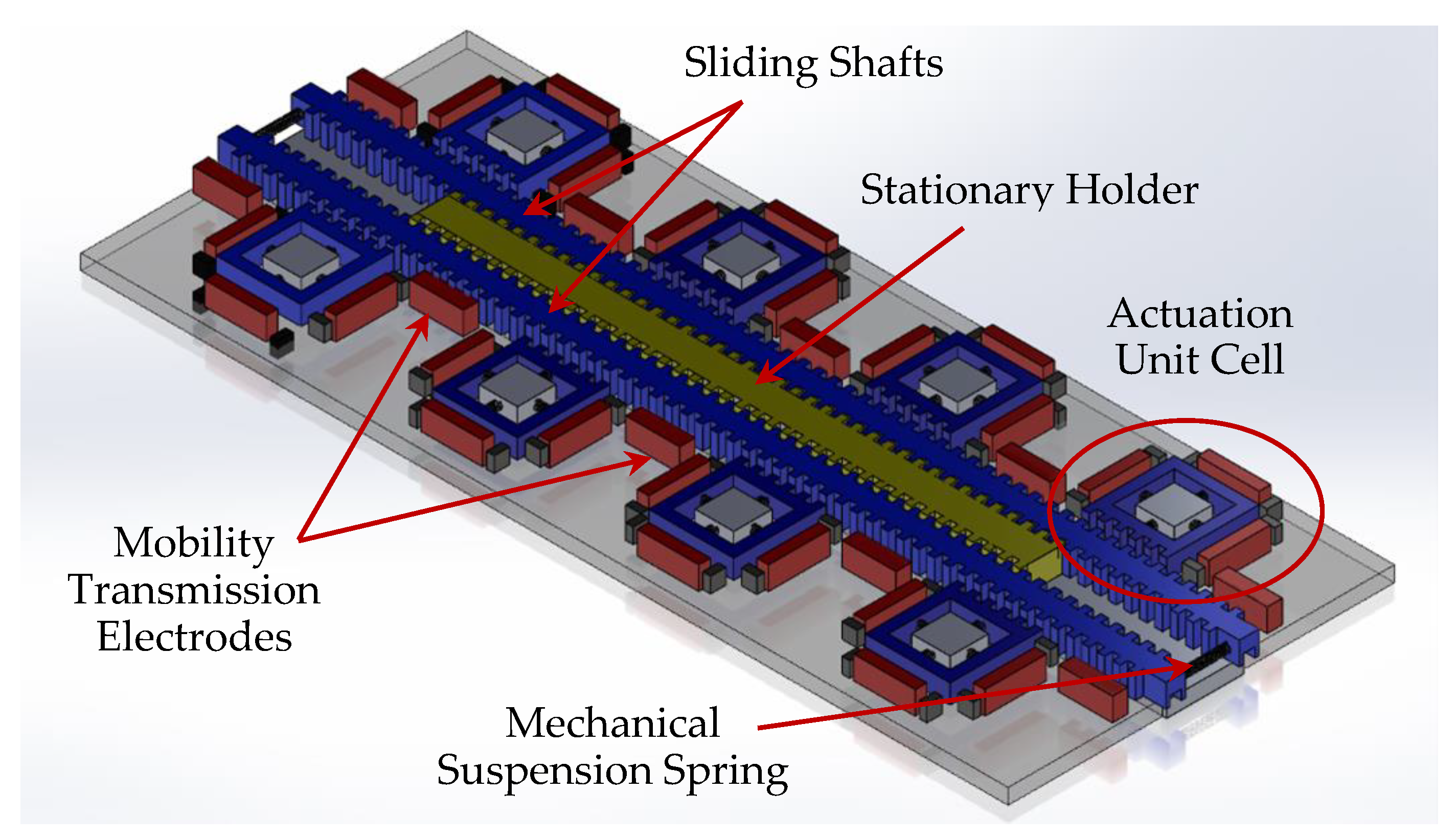
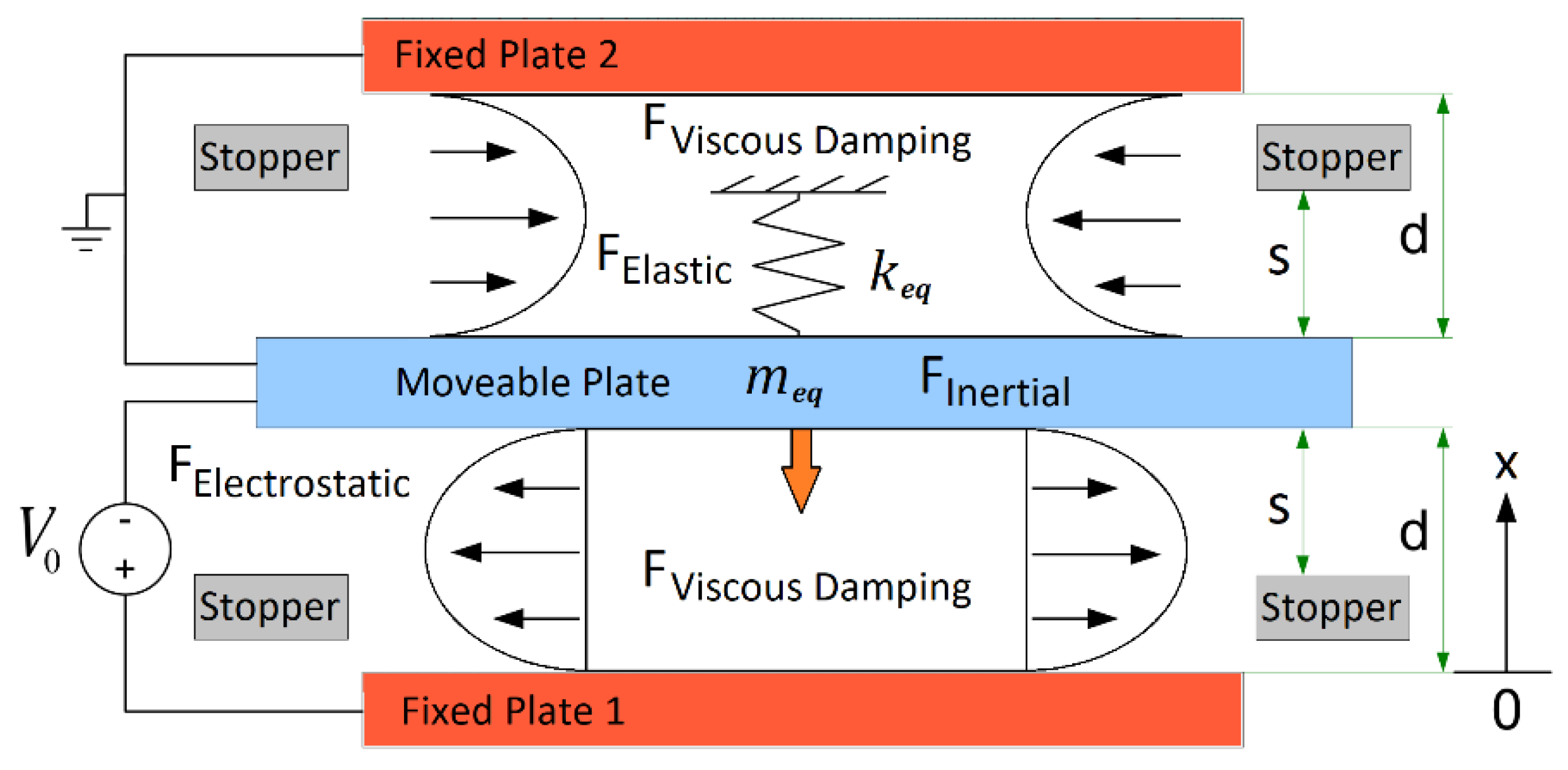
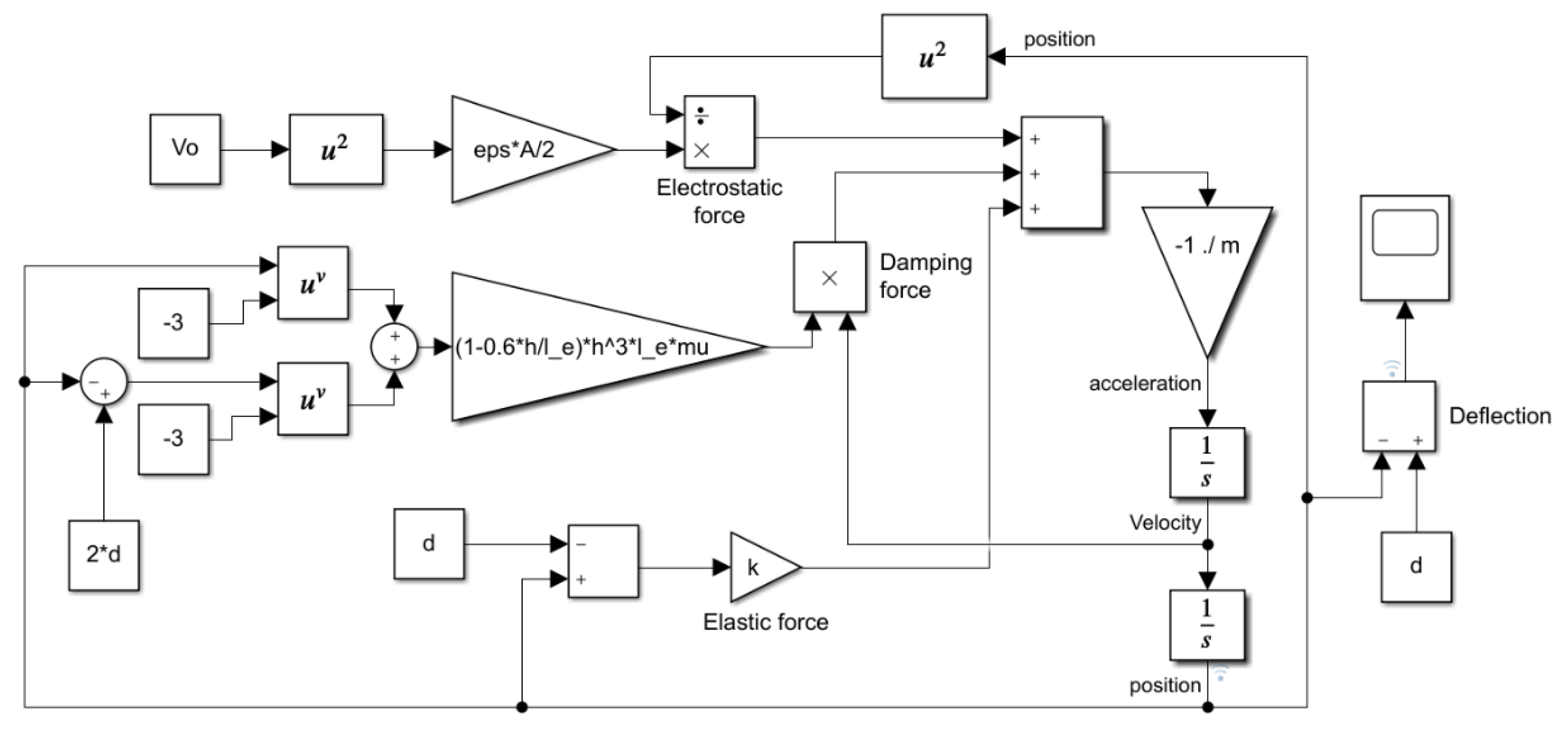
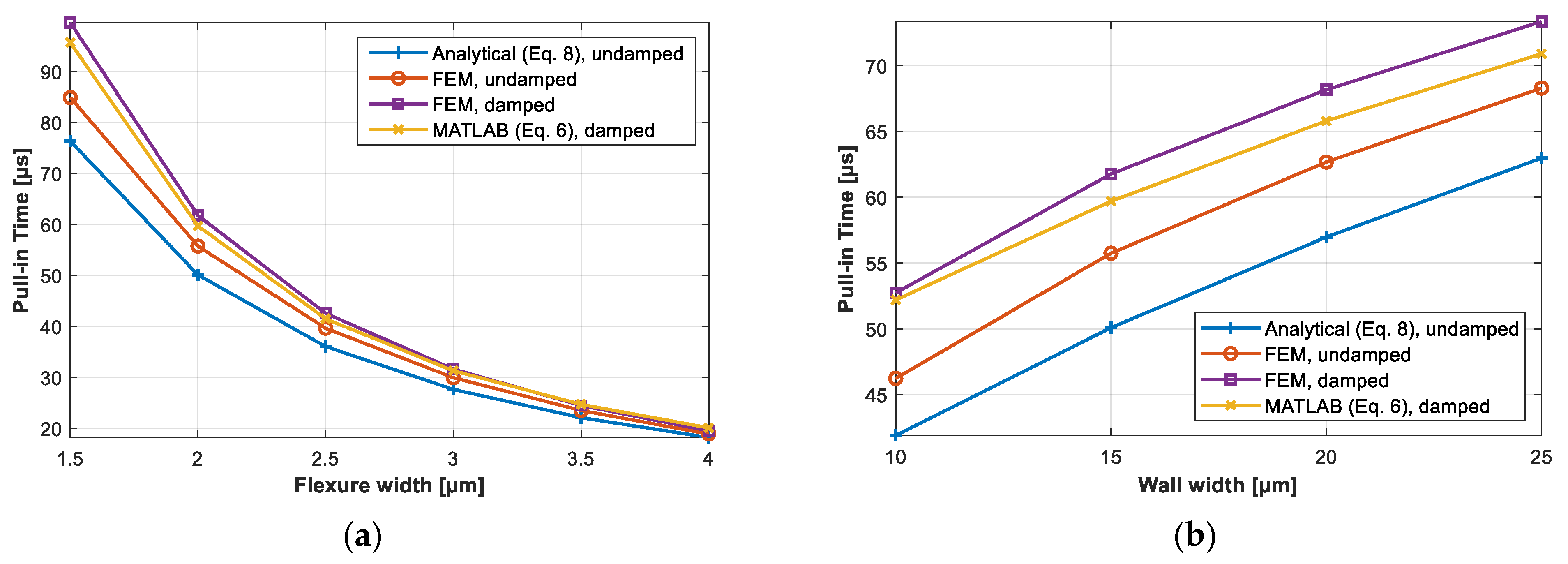
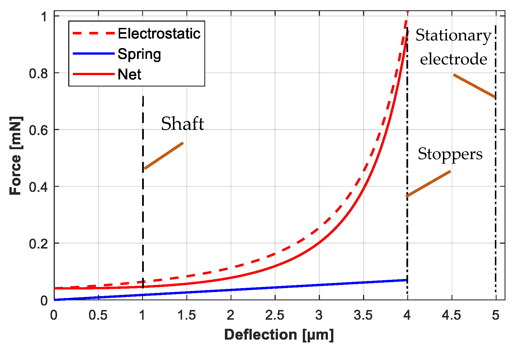
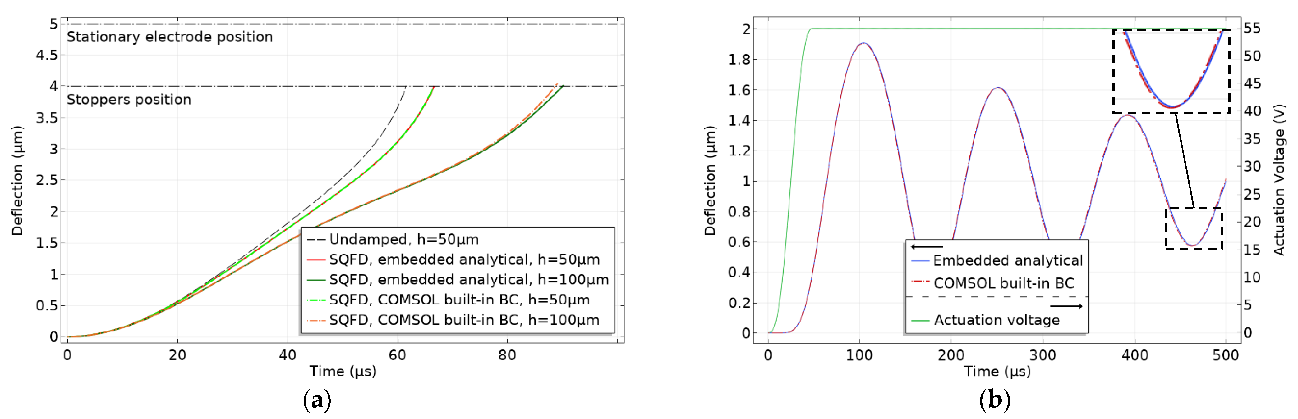
Table 1.
Typical parameter values for the AUC in the FEM model.
| Description | Symbol | Value | Unit |
|---|---|---|---|
| Height of unit cell | h | 50 | µm |
| Width of cell wall | ww | 15 | µm |
| Size of cell wall along x-axis (inner dimension) | cx | 500 | µm |
| Size of cell wall along y-axis (inner dimension) | cy | 500 | µm |
| Size of anchor (x-axis) | ax | 100 | µm |
| Size of anchor (y-axis) | ay | 100 | µm |
| Width of x-axis spring (flexure width) | wx | 2 | µm |
| Width of y-axis spring (flexure width) | wy | 2 | µm |
| Length of connector beams of x-axis spring | lc,x | 50 | µm |
| Length of span beam of x-axis spring | ls,x | 200 | µm |
| Length of extension beams of x-axis spring | le,x | 53 | µm |
| Length of connector beams of y-axis spring | lc,y | 50 | µm |
| Length of span beam of y-axis spring | ls,y | 200 | µm |
| Length of extension beams of y-axis spring | le,y | 53 | µm |
| Length of stationary electrodes | le | 460 | µm |
| Width of stopper (length of contact area) | ws | 25 | µm |
| Nominal air gap between electrodes | d | 5 | µm |
| Stroke (distance between mov. electrode at rest and stopper) | s | 4 | µm |
| Young’s modulus | E | 170 | GPa |
| Poisson’s ratio | ν | 0.28 | - |
| Density (c-Si) | ρ | 2329 | kg/m3 |
| Air viscosity | µ | 1.845 × 10⁻⁵ | Pa.s |
| Actuation Voltage | Vo | variable | V |
Table 2.
Examples of proposed AUC geometries for fabrication and their estimated performance characteristics. Absent AUC parameters have the same values as those listed in Table 1.
Table 2.
Examples of proposed AUC geometries for fabrication and their estimated performance characteristics. Absent AUC parameters have the same values as those listed in Table 1.
| Description | Symbol | Device 1 | Device 2 | Unit |
|---|---|---|---|---|
| Height of unit cell | h | 50 | 100 | µm |
| Width of cell wall | ww | 25 | 35 | µm |
| Size of cell wall (inner) | cx and cy | 500 | 600 | µm |
| Size of anchor | ax and ay | 100 | 100 | µm |
| Width of spring (flexure width) | wx and wy | 2.5 | 5 | µm |
| Length of connector beams | lc,x and lc,y | 50 | 50 | µm |
| Length of span beams | ls,x and ls,y | 200 | 300 | µm |
| Length of extension beams | le,x and le,y | 53 | 82.5 | µm |
| Length of stationary electrodes | le | 480 | 600 | µm |
| Width of stopper | ws | 25 | 25 | µm |
| Nominal air gap between electrodes | d | 5 | 4 | µm |
| Stroke | s | 4 | 3 | µm |
| Equivalent mass (assuming r = 0.5) | meq | 6.46 | 22.65 | µg |
| Equivalent spring constant 1 | keq | 40.4 | 304.8 | N/m |
| Pull-in voltage 1 | Vpull-in | 83.9 | 104.3 | V |
| Collapse voltage (2nd pull-in) 1 | Vcollapse | 152.0 | 165.9 | V |
| Actuation voltage | Vo | 110 | 130 | V |
| Pull-in time (corresponding to Vo) 2 | tpull-in | 32.2 | 24.9 | µs |
| Net force of AUC (at 1µm) 2,3 | F | 0.04 | 0.19 | mN |
| Net force of AUC (at 2µm) 2,3 | F | 0.06 | 0.51 | mN |
| Realignment margin | δ | ±2 | ±1 | µm |
| Pull-out time (corresponding to δ) 2 | tpull-out | 283 | 91 | µs |
1 Estimation based on static analysis in COMSOL 2D model. 2 Rough estimation based on MATLAB lumped-parameter model. 3 Damping force is neglected; the distance is from the undeflected position to the shaft (Figure 11).
Publisher’s Note: MDPI stays neutral with regard to jurisdictional claims in published maps and institutional affiliations. |
© 2021 by the authors. Licensee MDPI, Basel, Switzerland. This article is an open access article distributed under the terms and conditions of the Creative Commons Attribution (CC BY) license (https://creativecommons.org/licenses/by/4.0/).
Share and Cite
MDPI and ACS Style
Albukhari, A.; Mescheder, U. Investigation of the Dynamics of a 2-DoF Actuation Unit Cell for a Cooperative Electrostatic Actuation System. Actuators 2021, 10, 276. https://doi.org/10.3390/act10100276
AMA Style
Albukhari A, Mescheder U. Investigation of the Dynamics of a 2-DoF Actuation Unit Cell for a Cooperative Electrostatic Actuation System. Actuators. 2021; 10(10):276. https://doi.org/10.3390/act10100276
Chicago/Turabian StyleAlbukhari, Almothana, and Ulrich Mescheder. 2021. "Investigation of the Dynamics of a 2-DoF Actuation Unit Cell for a Cooperative Electrostatic Actuation System" Actuators 10, no. 10: 276. https://doi.org/10.3390/act10100276
Note that from the first issue of 2016, this journal uses article numbers instead of page numbers. See further details here.